Virtual concordance and the generalized Alexander polynomial
Hans U. Boden, Micah Chrisman

TL;DR
This paper links the generalized Alexander polynomial of virtual knots to welded links via the Zh-correspondence, demonstrating its functoriality under concordance and applying it to classify virtual knots by slice genus and sliceness.
Contribution
It establishes the functoriality of the Zh-map and Tube map under concordance, extending classical link group results to virtual knots, and applies these to classify virtual knots by sliceness.
Findings
The generalized Alexander polynomial vanishes on knots concordant to homologically trivial knots.
The polynomial vanishes on virtually slice knots.
Complete calculation of slice genus for certain virtual knots.
Abstract
We use the Bar-Natan Zh-correspondence to identify the generalized Alexander polynomial of a virtual knot with the Alexander polynomial of a two component welded link. We show that the Zh-map is functorial under concordance, and also that Satoh's Tube map (from welded links to ribbon knotted tori in ) is functorial under concordance. In addition, we extend classical results of Chen, Milnor, and Hillman on the lower central series of link groups to links in thickened surfaces. Our main result is that the generalized Alexander polynomial vanishes on any knot in a thickened surface which is concordant to a homologically trivial knot. In particular, this shows that it vanishes on virtually slice knots. We apply it to complete the calculation of the slice genus for virtual knots with four crossings and to determine non-sliceness for a number of 5-crossing and 6-crossing virtual knots.
Click any figure to enlarge with its caption.
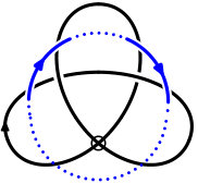 Figure 1
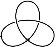 Figure 2
 Figure 3
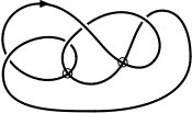 Figure 4
 Figure 5
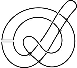 Figure 6
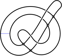 Figure 7
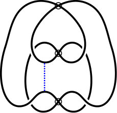 Figure 8
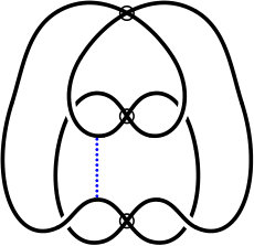 Figure 9
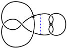 Figure 10
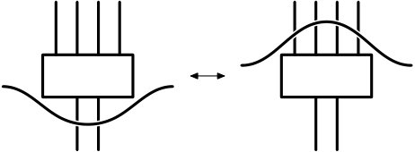 Figure 11
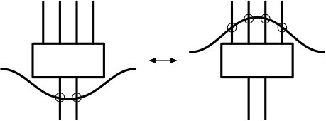 Figure 12
 Figure 13
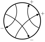 Figure 14
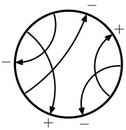 Figure 15
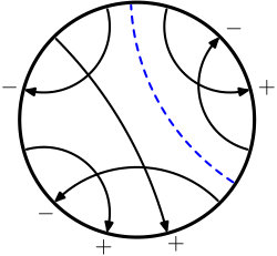 Figure 16
 Figure 17
 Figure 18
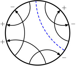 Figure 19
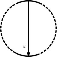 Figure 20
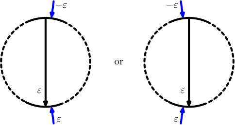 Figure 21
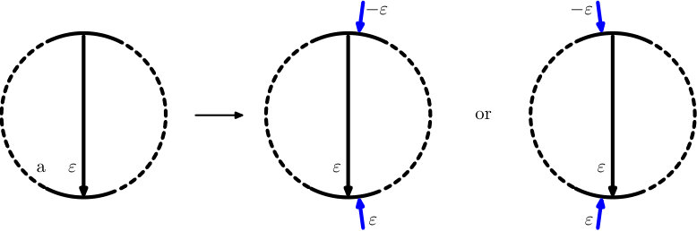 Figure 22
 Figure 23
 Figure 24
 Figure 25
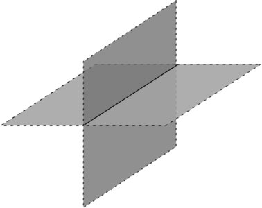 Figure 26
 Figure 27
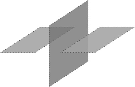 Figure 28
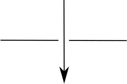 Figure 29
 Figure 30
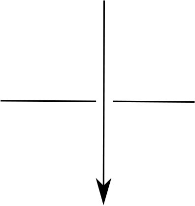 Figure 31
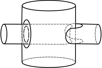 Figure 32
 Figure 33
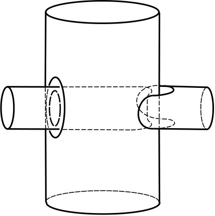 Figure 34
 Figure 35
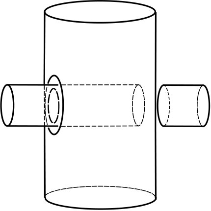 Figure 36
 Figure 37
 Figure 38
 Figure 39
 Figure 40
| Virtual | Generalized | Rasmussen | |
|---|---|---|---|
| knot | Gauss code | Alexander polynomial | invariant |
| 4.12 | O1-O2-U1-O3+U2-O4+U3+U4+ | ||
| 5.93 | O1-O2-U1-U2-U3+O4+O3+U5+U4+O5+ | ||
| 5.114 | O1-O2-U1-U2-U3+U4-O3+U5+O4-O5+ | ||
| 5.212 | O1-O2-U1-O3-U2-O4+U5+U3-O5+U4+ | ||
| 5.344 | O1-O2+U1-O3-U2+U4+O5+O4+U5+U3- | ||
| 5.919 | O1-O2-U1-O3+U4+U2-O5+U3+O4+U5+ | ||
| 5.1034 | O1-O2+U1-O3-U4+U3-O5-U2+O4+U5- | ||
| 5.1216 | O1-O2+U1-O3-U4+O5-O4+U2+U5-U3- | ||
| 5.1963 | O1-O2-O3-U1-U2-U4+O5+U3-O4+U5+ | ||
| 5.2351 | O1-O2-U3+O4+U1-U2-O5-U4+O3+U5- | ||
| 5.2430 | O1-U2-O3+U1-O2-U4-O5+U3+O4-U5+ | ||
| 5.2435 | O1-U2-O3-U1-O4+U3-O5+U4+O2-U5+ |
| Crossing | Virtual | combined | slice | status | |
|---|---|---|---|---|---|
| number | knots | sieve | sieve | knots | unknown |
| 2 | 1 | 0 | 0 | 0 | 0 |
| 3 | 7 | 1 | 0 | 0 | 0 |
| 4 | 108 | 15 | 14 | 13 | 0 |
| 5 | 2448 | 59 | 51 | 45 | 2 |
| 6 | 90235 | 1476 | 1294 | 1241 | 39 |
Peer Reviews
No public reviews on file for this paper yet. If you reviewed it on a platform where reviews are public (OpenReview, ICLR, NeurIPS, ICML), you can paste yours below so the community can read it here.
Videos
No videos yet. Explain this paper in a talk, walkthrough, or lecture? Add one.
Virtual concordance and the
generalized Alexander polynomial
Hans U. Boden
Mathematics & Statistics, McMaster University, Hamilton, Ontario
[email protected] https://www.math.mcmaster.ca/ boden and
Micah Chrisman
Mathematics, The Ohio State University, Columbus, Ohio
[email protected] https://micah46.wixsite.com/micahknots
Abstract.
We use the Bar-Natan Zh-correspondence to identify the generalized Alexander polynomial of a virtual knot with the Alexander polynomial of a two component welded link. We show that the Zh-map is functorial under concordance, and also that Satoh’s Tube map (from welded links to ribbon knotted tori in ) is functorial under concordance. In addition, we extend classical results of Chen, Milnor, and Hillman on the lower central series of link groups to links in thickened surfaces. Our main result is that the generalized Alexander polynomial vanishes on any knot in a thickened surface which is virtually concordant to a homologically trivial knot. In particular, this shows that it vanishes on virtually slice knots. We apply it to complete the calculation of the slice genus for virtual knots with four crossings and to determine non-sliceness for a number of 5-crossing and 6-crossing virtual knots.
Key words and phrases:
Virtual knot, slice knot, concordance, generalized Alexander polynomial, ribbon torus link, lower central series, boundary link
2010 Mathematics Subject Classification:
Primary: 57M25, Secondary: 57M27
The first author was partially funded by the Natural Sciences and Engineering Research Council of Canada, and the second author was partially funded by The Ohio State University.
1. Introduction
A knot in is called slice if it bounds a smoothly embedded disk in . Many classical knot invariants take a special form on slice knots. For instance, the knot signature vanishes, the determinant is a square integer, and the Alexander polynomial factors as for some integral polynomial. (The last one is the famous Fox-Milnor condition.)
In this paper, we study virtual knots and establish a similar condition on the generalized Alexander polynomial for slice virtual knots. The generalized Alexander polynomial first appeared in the work of Jaeger, Kauffman, and Saleur. In [JKS-1994] they introduce a determinant formulation for the Alexander-Conway polynomial derived from the free fermion model in statistical mechanics. Their approach involves constructing link invariants via partition functions and solutions to the Yang-Baxter equation. Using a particular solution, they derive an invariant of knots in thickened surfaces which takes the form of a Laurent polynomial in two variables. In the planar case, the invariant can be further normalized to give the classical Alexander-Conway polynomial.
In subsequent work, Sawollek [saw] observed that the approach of [JKS-1994] leads to a well-defined invariant of oriented virtual knots and links now known as the generalized Alexander polynomial. Virtual knots were introduced by Kauffman in the mid 1990s, and they can be viewed as knots in thickened surfaces up to isotopy, diffeomorphism, and stabilization, described in more detail in §2. The generalized Alexander polynomial plays a prominent role in virtual knot theory and can be interpreted in a variety of ways. It can be expressed as the zeroth elementary ideal of the extended Alexander group [Silver-Williams-2003], in terms of quandles [Kauffman-Radford, Manturov2002] and virtual biquandles [Crans-Henrich-Nelson], and as the Alexander invariant of the virtual knot group [Boden-Dies-Gaudreau-2015]. It has numerous applications: it can detect non-invertibility and non-classicality [saw, Silver-Williams-2003]; it gives a lower bound on the virtual crossing number [Boden-Dies-Gaudreau-2015]; and it dominates the writhe polynomial [Mellor-2016].
A knot in a thickened surface is said to be virtually slice if it bounds a smooth 2-disk in , where is a compact oriented -manifold with . There is much computational evidence suggesting that the generalized Alexander polynomial is a slice obstruction for virtual knots (see [Boden-Chrisman-Gaudreau-2017, Conj. 4.1]). Our main theorem confirms this conjecture by showing that the generalized Alexander polynomial vanishes on knots in thickened surfaces which are virtually concordant to homologically trivial knots (see Theorem 4.9). In particular, it follows that the generalized Alexander polynomial vanishes on virtually slice knots.
In §2, we introduce some basic notions and sketch the argument of the main result. In §3, we introduce virtual boundary links, and we give virtual analogues of results of Milnor [milnor, Theorem 4] and Hillman [hill]. In §4, we present the Zh-construction (due to Bar-Natan) and describe the Tube construction (due to Satoh). Both are shown to be functorial under concordance. The main result and its proof are given in §4.3, and applications to obstructing sliceness are given in §4.4. The paper concludes with §4.5, a brief discussion on further questions about the generalized Alexander polynomial and the Zh-construction.
2. Preparations
2.1. Basic Notions
We briefly review the basic notions of virtual knot theory, including virtual knot diagrams, welded equivalence, the link group, Gauss diagrams, and knots in thickened surfaces. For a thorough introduction, we recommend [Kauffman-1999]. Note that all virtual knots and links in this paper will be oriented.
A virtual knot diagram is an immersion of a circle in the plane whose double points are either classical (indicated by over- and undercrossings) or virtual (indicated by a circle). Figure 1 shows the virtual knot . The decimal number refers to the virtual knot table [Green]. Virtual link diagrams are defined similarly. Two such diagrams are virtually equivalent if they are related by planar isotopies, (classical) Reidemeister moves, and the detour move (see Figure 2). These moves are known collectively as the generalized Reidemeister moves.
Two virtual links are said to be welded equivalent if they can be represented by diagrams related by a sequence of generalized Reidemeister moves and the forbidden overpass (see Figure 2).
Associated to any virtual knot diagram is a Gauss code, which is a word that records the over and undercrossing information and signs of the crossings as one goes around the knot. A Gauss diagram is a decorated trivalent graph that records the same information. Full details can be found in [Kauffman-1999], and Figure 1 gives an illustrative example. Similar considerations apply to virtual link diagrams. There is a notion of equivalence of Gauss diagrams generated by generalized Reidemeister moves, and one can define virtual knots and links as equivalence classes of Gauss diagrams.
One can alternatively define virtual links as links in thickened surfaces up to stable equivalence. Let be a compact, connected, oriented surface. A link in is a 1-dimensional submanifold with finitely many components, each of which is homeomorphic to Stabilization is the addition or removal of a 1-handle to disjoint from the diagram of . Specifically, given disks disjoint from one another and from the projection of under , we set , where the 1-handle is attached along . This operation is called stabilization, and the opposite procedure, which is the removal of a 1-handle disjoint from , is called destabilization. Two links and are said to be stably equivalent if one is obtained from the other by a finite sequence of isotopies, oriented diffeomorphisms of , stablizations, and destablizations. By [Carter-Kamada-Saito], a virtual link is uniquely determined by the associated stable equivalence class of links in thickened surfaces, and vice versa.
A link is said to have minimal genus if it cannot be destabilized. On [kuperberg], Kuperberg proved that any two minimal genus representatives for the same virtual link are equivalent up to isotopy and diffeomorphism.
2.2. Generalized Alexander polynomial
In [saw], Sawollek introduced the generalized Alexander polynomial, an invariant of oriented virtual links. His definition is an adaptation of work of Jaeger, Kauffman and Saleur [JKS-1994], who extended the Alexander-Conway polynomial to links in thickened surfaces. Using the extended Alexander group, Silver and Williams defined Alexander invariants for virtual links [Silver-Williams-2001], and in [Silver-Williams-2003], they showed how to interpret Sawollek’s polynomial as the zeroth order Alexander invariant of their extended Alexander group. The resulting invariant will be denoted . We recall its definition from [Mellor-2016, Silver-Williams-2003]. (Note that we use variables in place of , respectively.)
Suppose is a virtual knot, represented as a virtual knot diagram with classical crossings. Fix an ordering of the crossings, and use it to determine an ordering on the short arcs of the diagram as follows. The short arcs start at one classical crossing and end at the next classical crossing, passing through any virtual crossings along the way. The ordering on the short arcs is chosen so that, at the -th crossing, the incoming short arcs are and , as depicted in Figure 3.
Define to be the block diagonal matrix with the blocks placed along the diagonal. Here is the matrix corresponding to the -th crossing, and it is equal to
[TABLE]
depending on the writhe of the -th crossing; namely we use if the writhe is positive and if it is negative.
The sequence of short arcs that are encountered as one travels along the knot determines a permutation of , given as a cycle. Let denote the associated permutation matrix; its entry is equal to 0 unless precedes as consecutive short arcs, in which case the entry equals 1. The generalized Alexander polynomial is then given by , and it is an invariant of the virtual link up to multiplication by powers of .
Example 2.1*.*
For the virtual knot in Figure 1, one can compute that its generalized Alexander polynomial is given by .
In [Silver-Williams-2001], Silver and Williams defined a multi-variable generalized Alexander polynomial. For a virtual link with components, we will denote their invariant by . Note that we use variables in place of (cf. [Silver-Williams-2001, §4]).
Using a simple change of variables, Silver and Williams showed that vanishes whenever is classical (see [Silver-Williams-2001, Corollary 4.3]). In [Silver-Williams-2006, §4], they extended this vanishing result to include almost classical links. Recall that a virtual link is said to be almost classical if some diagram of it admits an Alexander numbering [Silver-Williams-2006, Definition 4.1]. Note further that a virtual link is almost classical if and only if it can be represented as a homologically trivial link in a thickened surface (see [acpaper, Theorem 6.1]).
The vanishing result for can also be deduced Theorem 5.2 [acpaper]. In §4.1, we will give a new proof that the generalized Alexander polynomial vanishes for almost classical links, and in §4.3, we strengthen the statement and show that the generalized Alexander polynomial vanishes for any virtual knot that is concordant to an almost classical knot.
2.3. Virtual link groups
Suppose is a virtual link diagram with components . Suppose further that the -th component has undercrossings for thus has a total of crossings. We will label the arcs of according to the following scheme.
Fix a base point on that is not a crossing point, and starting at the base point, label the arcs consecutively so that contains the basepoint and so that and are the incoming and outgoing undercrossing arcs, respectively, at the -th undercrossing (see Figure 4). At the last crossing of , will be the incoming undercrossing arc and will be the outgoing undercrossing arc. Thus, we take modulo . Let be the overcrossing arc at this crossing, and let be the sign of the crossing. Notice that and are both functions of and , but we suppress their dependence here.
Definition 2.2**.**
The link group is the group with generators for and , and with relations given by the presentation
[TABLE]
This group is invariant under the generalized Reidemeister moves and the forbidden overpass, and consequently it is an invariant of the welded type of (see [Kim-2000]).
For virtual links represented instead as links in thickened surfaces, the link group is the fundamental group of the space obtained from by collapsing to a point (see [Kamada-Kamada-2000, Proposition 5.1]).
Given a link group for an oriented link with components, a choice of meridians determines an epimorphism with kernel , the commutator subgroup. Setting , we regard the quotient as a module over the group ring .
This module is of course just the Alexander invariant of , and using Fox differentiation one can easily describe it in terms of a presentation matrix called the Alexander matrix. For instance, for the group presentation (1), the Alexander matrix is the matrix with entry given by where is the relation The -th elementary ideal is denoted and defined to be the ideal generated by all the minors of for . For we set
The virtual link group was introduced in [Boden-Dies-Gaudreau-2015], and the virtual Alexander polynomial, denoted , is an invariant derived from the zeroth elementary ideal of the virtual Alexander invariant of (see [Boden-Dies-Gaudreau-2015, Definition 3.1]). It is closely related to the generalized Alexander invariant. Indeed, Proposition 3.8 of [Boden-Dies-Gaudreau-2015] implies that up to powers of and . The virtual Alexander polynomial also admits a normalization, which is denoted and well-defined up to powers of , and Proposition 5.5 of [Boden-Dies-Gaudreau-2015] implies that the normalized version satisfies . Thus the virtual Alexander polynomial determines the generalized Alexander polynomial and vice versa.
Next, we introduce the reduced virtual link group \hbox{ \kern-1.99997pt\vbox{\hrule height=0.5pt\kern 1.07639pt\hbox{\kern-1.49994ptG\kern-0.50003pt}}\kern 0.50003pt}_{L}. In §4, we will use the Bar-Natan Zh-construction to relate \hbox{ \kern-1.99997pt\vbox{\hrule height=0.5pt\kern 1.07639pt\hbox{\kern-1.49994ptG\kern-0.50003pt}}\kern 0.50003pt}_{L} to the link group of the welded link .
Definition 2.3**.**
Given a virtual link represented as a virtual link diagram , one can associate a finitely generated group with one generator for every short arc of , together with one auxiliary generator and one relation for each classical crossing of as given in Figure 5.
The resulting finitely presented group is an invariant of the virtual link and is denoted \hbox{ \kern-1.99997pt\vbox{\hrule height=0.5pt\kern 1.07639pt\hbox{\kern-1.49994ptG\kern-0.50003pt}}\kern 0.50003pt}_{L} (see [acpaper, Section 3] for a proof of invariance). It is called the reduced virtual link group.
We have chosen to use right-handed meridians here, and for that reason the isomorphism between the presentations of \hbox{ \kern-1.99997pt\vbox{\hrule height=0.5pt\kern 1.07639pt\hbox{\kern-1.49994ptG\kern-0.50003pt}}\kern 0.50003pt}_{L} and the one given in [acpaper] involves taking the inverses of the generators The auxiliary generator is unchanged.
The group obtained from \hbox{ \kern-1.99997pt\vbox{\hrule height=0.5pt\kern 1.07639pt\hbox{\kern-1.49994ptG\kern-0.50003pt}}\kern 0.50003pt}_{L} by taking is isomorphic to the link group [acpaper, §2].
Example 2.4*.*
For the virtual knot in Figure 1, one can compute that its knot group is cyclic, and that its reduced virtual knot group \hbox{ \kern-1.99997pt\vbox{\hrule height=0.5pt\kern 1.07639pt\hbox{\kern-1.49994ptG\kern-0.50003pt}}\kern 0.50003pt}_{K} is generated by two elements with a single relation:
[TABLE]
By [acpaper, Theorem 3.1], it follows that VG_{L}\cong\hbox{ \kern-1.99997pt\vbox{\hrule height=0.5pt\kern 1.07639pt\hbox{\kern-1.49994ptG\kern-0.50003pt}}\kern 0.50003pt}_{L}*_{\mathbb{Z}}{\mathbb{Z}}^{2}, thus the virtual link group can be recovered from \hbox{ \kern-1.99997pt\vbox{\hrule height=0.5pt\kern 1.07639pt\hbox{\kern-1.49994ptG\kern-0.50003pt}}\kern 0.50003pt}_{L}. Consequently, the Alexander invariants of these two groups are equivalent. The reduced Alexander polynomial \hbox{ \kern-1.99997pt\vbox{\hrule height=0.5pt\kern 1.07639pt\hbox{\kern-1.49994ptH\kern-0.50003pt}}\kern 0.50003pt}_{K}(s,t) is defined in [acpaper, §4] as the zeroth Alexander polynomial associated to the reduced virtual Alexander invariant \hbox{ \kern-1.99997pt\vbox{\hrule height=0.5pt\kern 1.07639pt\hbox{\kern-1.49994ptG\kern-0.50003pt}}\kern 0.50003pt}_{L}^{\prime}/\hbox{ \kern-1.99997pt\vbox{\hrule height=0.5pt\kern 1.07639pt\hbox{\kern-1.49994ptG\kern-0.50003pt}}\kern 0.50003pt}_{L}^{\prime\prime}. It is defined to be the generator of the smallest principal ideal containing \hbox{ \kern-1.99997pt\vbox{\hrule height=0.5pt\kern 1.07639pt\hbox{\kern-1.49994pt\mathscr{E}\kern-0.50003pt}}\kern 0.50003pt}_{0}, the zeroth elementary ideal. Then [acpaper, Theorem 4.1] implies that \hbox{ \kern-1.99997pt\vbox{\hrule height=0.5pt\kern 1.07639pt\hbox{\kern-1.49994ptH\kern-0.50003pt}}\kern 0.50003pt}_{K}(s,t) determines the generalized Alexander polynomial and vice versa.
2.4. Concordance
In this section, we introduce two equivalent notions of concordance for links in thickened surfaces and for virtual links, one is due to Turaev [Turaev-2008] and the other to Kauffman [Kauffman-2015]. We present several examples of virtual knots that are slice, and one that shows that the generalized Alexander polynomial is not, in general, invariant under virtual concordance. At the end, we define welded link concordance.
In general, two links in a 3-manifold are said to be cobordant if they cobound a properly embedded oriented surface in the cylinder They are said to be concordant if, in addition, the cobordism surface can be chosen to be a disjoint union of annuli.
In the case is a thickened surface , there are more relaxed notions that are called virtual cobordism and virtual concordance. They were first introduced by Turaev [Turaev-2008], and they provide the added flexibility of allowing the surface to change by cobordism.
Definition 2.5**.**
Two oriented links and in thickened surfaces are said to be virtually cobordant if there exist a compact oriented 3-manifold with , together with an oriented surface smoothly and properly embedded in with .
The links and are said to be virtually concordant if, in addition, the surface is a disjoint annuli, each with one boundary component on and the other on .
The above definitions can be easily translated into the language of virtual links. For instance, two virtual links are said to be cobordant if they can be represented by links in thickened surfaces that are virtually cobordant, and likewise for concordance.
In [Kauffman-2015], Kauffman introduced an equivalent description for cobordism and concordance of virtual links. His definition is purely diagrammatic and is given in terms of finding a sequence of births, deaths, and saddle moves.
A birth is the addition of a trivial unknotted unlinked component and a death is the removal of a trivial unknotted unlinked component. A saddle is a move that cuts and rejoins two arcs in a way that respects their orientations, see Figure 6. Given a cobordism, its Euler number is defined to be , where is the number of births, is the number of deaths, and is the number of saddles. The genus of the cobordism surface is determined from its Euler characteristic in the usual way.
Definition 2.6**.**
Two virtual links and are said to be cobordant if they have the same number of components and can be represented by virtual link diagrams that are related to one another by a finite sequence of moves that include generalized Reidemeister moves, together with births, deaths, and saddles.
Further, two virtual links and are said to be concordant if there exists a sequence of generalized Reidemeister moves and births, deaths, and saddles which take to and satisfy for each . A virtual link that is concordant to the unlink is called slice.
Remark 2.7*.*
(i) Note that cobordant virtual links are required to have the same number of components. Likewise for concordance.
(ii) Cobordism determines an equivalence relation on virtual links. The pairwise virtual linking numbers of the components are invariant under virtual link cobordism. Concordance also determines an equivalence relation on virtual links which is of course a refinement of cobordism.
(iii) Any two virtual knots are cobordant, in particular, any virtual knot is cobordant to the unknot (see [Kauffman-2015]). The slice genus of a virtual knot is denoted and is defined to be the minimum genus over all cobordisms from to the unknot.
A proof that Definitions 2.5 and 2.6 are equivalent for virtual links was given by Carter, Kamada, and Saito [Carter-Kamada-Saito-2004]. In these terms, they prove that two links in thickened surfaces are virtually concordant if and only if they represent concordant virtual links.
As for classical knots, sliceness and concordance is most easily described via a slice movie where one shows the saddles, births and deaths diagrammatically. Suppose and are virtually concordant. Thus they represent concordant virtual links. By Definition 2.5, there exists an oriented 3-manifold with and an oriented surface with . One can view virtual concordance in terms of relative Morse theory as follows. A concordance movie gives rise to a Morse function on with for such that the restriction is also Morse. Critical points of correspond to stabilizations and destabilizations of the ambient surface. Local minima and maxima of correspond to births and deaths, respectively, and saddles of correspond to saddle moves. One can arrange the critical values of and to be disjoint by performing the generalized Reidemeister moves in between all births, deaths, and saddles. We give a few examples to illustrate this technique.
Example 2.8*.*
Satoh’s knot is depicted on the left of Figure 7. Performing a saddle along the dotted blue arc, one obtains the two-component virtual link on the right. Using generalized Reidemeister moves (actually type II only, both classical and virtual), this link is easily seen to be equivalent to the unlink of two components. Capping off one of the trivial components, one obtains a concordance from Satoh’s knot to the unknot. Thus, Satoh’s knot is seen to be slice.
The same method can be used to show sliceness for many other virtual knots. For example, consider the virtual knots 4.59 and 4.98 in Figure 8. Performing saddle moves along the dotted blue arcs and applying generalized Reidemeister moves, one can see that the resulting two component virtual links are trivial. Thus both virtual knots 4.59 and 4.98 in Figure 8 are slice.
This technique for slicing virtual knots has been adapted to Gauss diagrams, and it allows one to quickly and easily find slicings for a great many virtual knots [Boden-Chrisman-Gaudreau-2017].
There is a close relationship between concordance of virtual knots and connected sum. Recall that connected sum is not a well-defined operation on virtual knots; it depends on the diagrams used as well as the connection site. In fact, one can produce examples of nontrivial virtual knots by taking the connected sum of two virtual knot diagrams of the unknot. The Kishino knot is the most famous such example, and any virtual knot like that is slice; just perform a saddle move across the isthmus of the connected sum and the resulting two component virtual link is obviously trivial. (Note that this argument works more generally for connected sums of slice virtual knots.)
In a similar way, one can show that the virtual knots and are concordant whenever is slice. (This statement is independent of the indeterminacy inherent to connected sum operation on virtual knots.)
For a specific example, consider the virtual knot pictured on the left in Figure 9. Performing a saddle along the dotted blue curve gives a concordance to the virtual knot 3.2, the virtual figure eight knot. (This is immediate from the fact that is the connected sum of with a virtual unknot.) It follows that the virtual knots and are concordant. Furthermore, by direct computation, one sees that their generalized Alexander polynomials are given by
[TABLE]
Since up to units in this example shows that the generalized Alexander polynomial is not invariant under concordance.
Going back to Definition 2.5, when the cobordism is a product, i.e. when , we say that the concordance is strict. More precisely, two links are said to be strictly concordant if there exists a disjoint union of annuli with . A link in that is strictly concordant to the trivial link is said to be strictly slice.
For links in thickened surfaces, strict concordance can be described in terms of saddles, births and deaths on a link diagram in the surface. However, because stabilization and de-stabilization of the surface is not permitted, strict concordance is considerably stronger than virtual concordance. For example, if are strictly concordant, then and are homologous in . In particular, if one of them is null-homologous, then the other one must also be. For example, if is a strictly slice knot, then is necessarily null-homotopic and therefore null-homologous.
On the other hand, there are many examples of knots in which are virtually slice but not homologically trivial. The simplest ones are obtained by taking a simple closed curve with homology class . As long as is non-trivial, then is not strictly slice, but it nevertheless represents the trivial virtual knot and hence is virtually slice.
More interesting examples can be obtained by taking a virtual knot that is slice but not almost classical. For instance, any of the knots from Figures 7 and 8. When represented as a knot in a thickened surface, one obtains a knot in a thickened surface of genus two which is virtually slice but not strictly slice. The same is true of any of the many virtual knots from [Boden-Chrisman-Gaudreau-2017] that are known to be slice but not almost classical.
We end this section with the definition of welded concordance.
Definition 2.9**.**
Two virtual links and are said to be welded concordant if there is a finite sequence of generalized Reidemeister moves, forbidden overpass moves, and births, deaths, and saddles, which satisfy and take take to for each .
Welded concordance gives an equivalence relation on virtual links which is coarser than virtual concordance. For example, any virtual knot is welded concordant to the unknot. In short, every welded knot is slice. This is not obvious, but it follows by a clever argument due to Gaudreau [Gaudreau-2019, Theorem 5].
2.5. Sketch of the proof
Our main result is Theorem 4.9. It states that the generalized Alexander polynomial vanishes for knots in thickened surfaces which are virtually concordant to homologically trivial knots. Below we give a brief sketch of the proof.
Given a virtual knot , we associate to it a two-component semi-welded link such that the (reduced) virtual knot group \hbox{ \kern-1.99997pt\vbox{\hrule height=0.5pt\kern 1.07639pt\hbox{\kern-1.49994ptG\kern-0.50003pt}}\kern 0.50003pt}_{K} is isomorphic to the classical link group It follows that their Alexander modules are isomorphic. Thus, they have the same elementary ideals up to an overall degree shift, which is the result of the fact that the number of meridional generators increases by one under the Zh-map. (Note that the elementary ideals of the virtual Alexander module \hbox{ \kern-1.99997pt\vbox{\hrule height=0.5pt\kern 1.07639pt\hbox{\kern-1.49994ptG\kern-0.50003pt}}\kern 0.50003pt}_{K}^{\prime}/\hbox{ \kern-1.99997pt\vbox{\hrule height=0.5pt\kern 1.07639pt\hbox{\kern-1.49994ptG\kern-0.50003pt}}\kern 0.50003pt}_{K}^{\prime\prime} are indexed as in [acpaper].) In particular, the isomorphism of Alexander modules identifies with for
Additionally, the correspondence is functorial with respect to concordance. Namely, if and are concordant as virtual knots, then and are concordant as welded links.
Next, we apply Satoh’s Tube map to the welded link (see §4 for more details), and consider the resulting ribbon torus link The Tube map is also shown to be functorial in concordance. That is, if and are concordant as welded links, then and are concordant as ribbon torus links.
A result of Stallings then shows that, for compact submanifolds of , the nilpotent quotients of the fundamental group of are invariant under concordance. Applied to since the classical link group is isomorphic to this implies that the nilpotent quotients of are invariant under concordance of the welded link
Any knot in a thickened surface represents a virtual knot . If is concordant to an almost classical knot, then the welded link is welded concordant to a virtual boundary link (see Definition 3.1 below). Therefore, the nilpotent quotients of G_{L}\cong\hbox{ \kern-1.99997pt\vbox{\hrule height=0.5pt\kern 1.07639pt\hbox{\kern-1.49994ptG\kern-0.50003pt}}\kern 0.50003pt}_{K} coincide with those of the free group on two generators. Using the Chen-Milnor presentation of the nilpotent quotients, we conclude that the longitudes of must lie in the nilpotent residual Applying a result of Hillman, suitably extended to virtual link groups, it follows that the first elementary ideal is trivial, and we conclude that the generalized Alexander polynomial of must vanish.
3. Classical results for virtual links
3.1. Virtual boundary links
In the following, is a closed oriented surface, and denotes the free group on generators.
Definition 3.1**.**
A link is called a boundary link if its components bound pairwise disjoint Seifert surfaces in . A virtual link that can be represented by a boundary link will be called a virtual boundary link.
Note that every virtual boundary link is almost classical, but the converse is not true for links with components. For links in thickened surfaces, the property of being a boundary link is not preserved under stabilization, but it is preserved under destabilization. This last fact can be proved using an argument similar to the proof of Theorem 6.4 in [acpaper]. Thus, given a virtual link, it is a virtual boundary link if and only if its minimal genus representative satisfies Definition 3.1. In particular, it follows that a classical link is a virtual boundary link if and only if it is a boundary link.
For a classical link with components, Smythe showed that is a boundary link if and only if there is an epimorphism mapping the set of meridians to a free basis [Smythe-1966]. This result was extended to higher dimensional links by Gutiérrez [Gutierrez-1972]. The next result gives the analogue in one direction for virtual links. Note that the other implication is not true for virtual links, in fact it fails already for virtual knots. In that case, the knot group always admits an epimorphism to but a virtual knot admits a Seifert surface if and only if it is almost classical. Thus, a virtual knot is a boundary link if and only if it is almost classical.
Proposition 3.2**.**
Suppose is a link in a thickened surface with link group . If is a boundary link with components, then there is an epimorphism mapping the set of meridians of to a free basis.
Proof.
Let , and set Since is a boundary link, we have a collection of pairwise disjoint surfaces in such that for . Let be disjoint open tubular neighborhoods of in . Since is homotopic to a 1-dimensional complex, it follows that for .
Let be a bouquet of circles, with basepoint the wedge point. Define as follows. For , let , the -th circle of . This defines on the union , and we extend to all of by sending points in to the basepoint . Obviously, the bouquet of circles is a , and maps the meridians of to a set that freely generates . Since , we conclude that gives an epimorphism sending the meridians of to a free basis for . ∎
Given a finitely generated group , let and denote the first and second commutator subgroups of .
The next result is an immediate consequence of Proposition 3.2 and Theorem 4.2 in [Hillman-2012], which asserts that whenever there is an epimorphism .
Corollary 3.3**.**
If is a boundary link with components and link group , then .
3.2. Lower central series
For a group , the lower central series is the descending series of normal subgroups defined inductively by and for . Set . The quotient is called the -th nilpotent quotient of and is called the nilpotent residual of .
The next theorem is a classical result due to Stallings, see [stallings_central, Theorem 3.4].
Theorem 3.4** (Stallings).**
Let be a homomorphism of groups inducing an isomorphism and a surjection . Then for finite , induces an isomorphism . If is onto, then also induces an isomorphism .
In the following, let be the free group on generators.
Theorem 3.5**.**
Suppose is a boundary link with components. Then for all finite , and . Further, every longitude of satisfies .
Proof.
The epimorphism of Proposition 3.2 clearly induces an isomorphism and a surjection . (Indeed, .) Thus, Theorem 3.4 applies to prove the first part.
To prove the second part, recall that finitely generated free groups are residually nilpotent, hence . Thus, showing that the longitudes of lie in is equivalent to showing they lie in the kernel of the epimorphism .
Recall the construction of the map of pointed spaces from the proof of Proposition 3.2. (Here and .)
Let be the -th component of , and be the longitude of . We choose a representative for which is a simple closed curve on the Seifert surface for . By pushing this curve in the positive normal direction to , we can arrange that it lies outside the open tubular neighborhood of . By construction, sends this curve to the basepoint , and it follows that . This completes the proof of the second part. ∎
3.3. The Chen-Milnor Theorem
Milnor described a presentation for the nilpotent quotients of the link group of a classical link in [milnor], and this was extended to virtual links in [dye_kauffman]. We present an alternative proof for virtual links based on the argument of Turaev [Turaev-1976].
Let be an oriented virtual link diagram with components. We regard the link group with its Wirtinger presentation as in Definition 2.2. For , we choose one arc on the -th component of and let denote the resulting meridian, which is given by the associated generator of (1). The corresponding longitude is the word obtained by following in the direction of its orientation, starting at the chosen arc, and at each undercrossing recording the overcrossing arc with sign according to the writhe of the crossing. The resulting word is multiplied by the appropriate power of so that the longitude has -th exponential sum equal to zero.
Theorem 3.6**.**
Let be a link with components and link group , and let be the free group generated by . Then has a presentation:
[TABLE]
where and represent the images in of the -th meridian and longitude, respectively.
Proof.
Write , and let be the union of disjoint tubular neighborhoods in . Each is a solid torus and has boundary .
Let be the exterior of in , and set . Notice that is homotopic to with a cone placed on top, and that . In the following, we choose the basepoint to lie on .
We choose arcs in from to whose interiors are disjoint and lie in . Let be a closed regular neighborhood of in , and notice that . Further, let , so that . Thus is a once-punctured torus.
Let and Clearly , with one generator for each meridian of . We claim that . To see this, notice that is a 3-manifold with two boundary components, one is and the other is the connected sum of with the tori connected along the tubes . Writing and using the long exact sequence for the pair , it follows that is generated by and subject to the single relation Thus , and since , it follows that as claimed.
One can construct a by attaching cells of dimension to , and the induced map is therefore surjective. Thus , and applying Theorem 3.4, we see that the inclusion of the meridians induces an isomorphism for all Since , it follows that the link group is isomorphic to the quotient where represents the commutator of curves in whose images in are the meridian and longitude of the -th component. This completes the proof. ∎
Proposition 3.7**.**
Let be a link with components and link group . Then if and only if all the longitudes of lie in the nilpotent residual .
Proof.
If the longitude lies in , then the corresponding element in the presentation of (2) necessarily lies in Consequently, if all the longitudes of lie in , then for . In particular, if for , then the relations are consequences of the relations . In that case, the presentation (2) of Theorem 3.6 simplifies to show that which proves one direction.
To prove the other direction, suppose conversely that for all . Then the relations of the presentation (2) must be consequences of the relation . Recall that the -th longitude is defined to have zero exponential sum with respect to the -th meridian, and so Corollary 5.12 (iii) of [Magnus-Karrass-Solitar] applies to show that since , we must have . Consequently, it follows that , and since this holds for all we conclude that . ∎
3.4. The Chen groups
Given a finitely generated group , define the Chen groups of to be the quotient groups
[TABLE]
Let .
The following result is the main theorem of [hill], extended slightly to include link groups of virtual links in part (3).
Theorem 3.8** (Hillman).**
If is a finitely presented group with , then the following conditions are equivalent.
- (1)
* (i.e. the first Alexander ideals vanish).* 2. (2)
For each integer , the -th Chen group of satisfies
[TABLE]
where is a free group of rank .
Further, if is a link group of a virtual link (see Definition 2.2), then (1) and (2) are equivalent to:
- (3)
The longitudes of are in
Proof.
The proof of equivalence of (1) and (2) can be found in [hill]. Our focus is on showing that (2) and (3) are equivalent for link groups of virtual links. To that end, suppose that is the link group of a link . Let denote the longitudes of .
(2) implies (3). This follows by the proof given in [hill].
(3) implies (2). Suppose that for . Let be the free group generated by . Then arguing as in Proposition 3.7, it follows that for all . Consider the following commutative diagram, where the vertical maps , and are induced by the homomorphism sending to a meridian for the -th component of .
[TABLE]
The two rows are exact, and and are isomorphisms. Therefore, is also an isomorphism, and it follows that for all . Thus, we see that (2) holds. ∎
4. Crossing the crossings and the tube construction
4.1. The Bar-Natan Zh-construction
In this section, all virtual links are assumed to be oriented, and Zh refers to the Cyrillic letter and is pronounced “zh”. This letter was chosen as a symbol for the operation of “crossing the crossings” [Dror].
Given a virtual link diagram , following [Dror], one can construct a new diagram as follows. If has components, then has components, it is obtained from by adding one new component, which is drawn in blue and includes two new overcrossings for each classical crossing of (see Figure 10). The new overcrossings are connected to one another, adding virtual crossings wherever needed to cross any existing arcs.
For a given virtual link diagram we write Here refers to the new component and is considered up to semi-welded equivalence, which is defined next.
Definition 4.1** (semi-welded equivalence).**
Let be a virtual link diagram with components Fix nonnegative integers with , and regard the components as regular (or virtual) components and the components as -components (or welded components). A semi-welded equivalence of is a sequence of moves which include generalized Reidemeister moves anywhere, and forbidden overpass moves only when the overcrossing arc belongs to one of the -components.
An elementary exercise shows that semi-welded equivalence induces an equivalence relation on virtual link diagrams. Further, if and are semi-welded equivalent, then they necessarily have the same number of regular components and the same number of -components. If then there are no -components, and semi-welded equivalence is just virtual equivalence. On the other hand, if , then every component is an -component, and semi-welded equivalence is just welded equivalence. In general, for any with , virtual equivalence implies semi-welded equivalence, and semi-welded equivalence implies welded equivalence.
In this paper, we will consider only semi-welded equivalence in the case where there is just one -component, namely the one arising from the Zh-construction. Henceforth, we will write “semi-welded equivalence” instead of “ semi-welded equivalence.”
One immediate consequence is that deleting the -component from simply returns the original link diagram . Furthermore, since the -component in consists exclusively of overcrossings, these crossings may be ordered without altering its semi-welded type. This follows essentially from the forbidden overpass move, as we now explain.
First, fix a basepoint and form a loop with the -component by connecting the overcrossing arcs in any fashion, introducing virtual crossings as needed to make the connections. This provides a way to order the crossings of the -component, albeit arbitrary. However, note that any two consecutive overcrossings of the -component can be transposed. If the two undercrossing arcs are adjacent to one another, this can been seen by performing a virtual Reidemeister two move and forbidden overpass move (see Figure 11). If the two undercrossing arcs are not adjacent, one can apply detour moves to arrange for them to be adjacent (see Figure 12).
Consequently, the semi-welded link type of is independent of the order chosen for the overcrossings of the -component. It is also independent of the choice of basepoint, which can be seen using detour moves. In Figure 10, the dotted curves illustrate a way to connect the overcrossings, but one could alternatively connect them in any other way without altering the underlying semi-welded link.
For any subset of crossings of the -component, one can draw a loop starting and ending at the basepoint. In that case, we say that the -component contains the loop.
Proposition 4.2** (Bar-Natan).**
The semi-welded link depends only on the virtual link of .
Proof.
Suppose and are two virtual link diagrams that are related by generalized Reidemeister moves, then we must show that and are semi-welded equivalent. It is enough to prove this in the case and are related by a single Reidemeister move.
To this end, Polyak’s result in [Polyak] shows that all the Reidemeister moves can be generated from the four moves and , so it is enough to prove invariance of under each one of these four moves.
The proof in the case of the move is shown in Figure 13. Notice that after performing a Reidemeister 2 move, there are no classical crossings on the -arc, which is why it appears dotted in the middle frame of Figure 13. As such, it can be erased altogether. The proof for the move is similar.
The argument for the move is shown in Figure 14. The first frame shows the -arc with four overcrossings, but they all eventually cancel out under successive Reidemeister 2 moves. Once the -arc can be drawn without classical crossings, it can be erased just as before.
The proof for the move is described in Figure 15. In the first frame, the -arc is seen to contain a loop around the three crossings. Notice that this loop can be drawn without any virtual crossings. Therefore, using the forbidden overpass, the loop can be pulled off. After performing a Reidemeister 3 move, one can then use the forbidden overpass to insert a loop going in the opposite direction. This shows invariance of the Zh-construction under the move and completes the proof. ∎
Figure 16 shows the result of applying the Zh-construction to the virtual trefoil, also known as the virtual knot , and in that figure all crossings along the dotted blue curves are virtual.
We now describe an alternative formulation of the Zh-construction in terms of Gauss diagrams which is sometimes useful. Suppose that is a Gauss diagram representing the virtual link . Then is the Gauss diagram with one extra component obtained by adding two new arrows (both overcrossings) to either side of each existing chord of . The new arrows are drawn in blue, and they comprise the -component. There are two possible configurations for the new arrows, as shown on the right of Figure 17, either before the foot and after the head of the existing chord, or after the foot and before the head. These two configurations are equivalent by a semi-welded RM3 move. The two new arrowheads have opposite sign; the one nearest the head of the existing chord has sign equal to that of the chord, and the one nearest the foot has the opposite sign. Since is considered up to semi-welded equivalence, the order of the new arrows is arbitrary. For that reason, we do not bother to draw the core circle for the -component. If one wants, one could degenerate the core circle of the new component to a point, reflecting the fact that the new arrows can be reordered arbitrarily.
One can use this approach to give an alternative proof of Proposition 4.2 in terms of Gauss diagrams. We leave the details as an entertaining exercise for the reader.
Proposition 4.3**.**
The Zh-construction is functorial under virtual link cobordism. Namely, given a cobordism between virtual link diagrams and , there is a cobordism between the semi-welded link diagrams and Furthermore, if the cobordism from to has births, deaths, and saddles, then the cobordism from to also has births, deaths, and saddles.
Proof.
Notice that a cobordism can be decomposed into a sequence of operations, each of which is one of the generalized Reidemeister moves or a birth, death, or saddle. We have already seen that the Zh-construction commutes with each of the generalized Reidemeister moves, so all that remains is to prove it commutes with births, deaths, and saddles.
Since the Zh-construction only affects the virtual link locally at the classical crossings, it follows that if is obtained from by a birth, death, or saddle, then is obtained from by the very same birth, death, or saddle.
It follows that if is a virtual link cobordism from to , then is a semi-welded link cobordism from to ∎
Observe that, from the above proof, it follows that the Euler number of the cobordism from to is equal to that of the cobordism from to .
Corollary 4.4**.**
If and are concordant virtual links, then and are concordant as semi-welded links.
In [Dror], Bar-Natan proves that the Zh-map “factors on -links,” which is to say that if is a classical link, then the -component is unknotted and unlinked. The next theorem shows that factors similarly for almost classical links.
Theorem 4.5**.**
If is an almost classical virtual link, then the -component is unknotted and unlinked and is semi-welded equivalent to the split almost classical link . In particular, if is a virtual boundary link, then is semi-welded equivalent to a virtual boundary link.
Proof.
In the proof of invariance under in Proposition 4.2, we showed that the -arc contains a loop without virtual crossings which can be pulled off. The same reasoning applies to any disk-like region bounded by arcs of a link diagram provided they are all oriented in the same direction.
This observation is a key step here, and to use it we claim that can be represented by a special kind of diagram on . A diagram on is called checkerboard colorable if the regions of can be colored black or white so that adjacent regions have opposite colors. One may further assume, by destabilizing if necessary, that is a union of disks.
A virtual link is almost classical if and only if it bounds a Seifert surface, and every almost classical link is checkerboard colorable (see [acpaper]). Given such a link, using isotopies, one can arrange that the black surface of the checkerboard coloring is a Seifert surface. This will be the case if and only if all crossing are type I crossings (see e.g. [Burde-Zieschang]), which means that the black regions, which are all disks, are the ones obtained by performing oriented smoothings at all crossings.
We therefore assume that is given as a checkerboard colored diagram where the black regions form a Seifert surface. Each black region is a disk and is oriented so that its boundary orientation agrees with the orientations of the arcs of the diagram that form its boundary. The crossings of the -arc are co-oriented with the arcs of the diagram (see Figure 18), and thus the crossings of the -arc around a black region induce the same orientation on it.
The black regions are partitioned into two subsets. One consists of the black regions with boundary oriented counterclockwise, and the other consists of the black regions whose boundary is oriented clockwise. (This reflects the well-known fact that the Tait graph of a Seifert surface is bipartite.) The following argument would work with either subset of black regions, but we phrase it in terms of counterclockwise oriented regions, which coincide with the regions to the left of the -arcs. The crossings of the -arc around any such region may be stitched together to form a loop. These loops bound disks, namely the black regions themselves. We claim that these loops can be pulled off.
To prove the claim, fix a black disk and project the surface onto the plane so that the disk is embedded. This can be achieved by shrinking the disk by an isotopy if necessary. The projection gives a virtual link diagram for which has no virtual crossings in the image of the disk. The -arc will then contain a loop going around the image disk, and notice that this loop will not contain any virtual crossings. Therefore, one can pull the loop off the disk, thereby eliminating its classical crossings. Repeat this argument for the other counterclockwise black regions. By the forbidden overpass move, the loops may be connected in any order to form the -component, where only virtual crossings are added between the loops. By successively pulling loops off their black discs, one can eliminate all the remaining classical crossings of the -arc. This shows that is split and the theorem follows. ∎
For the next result, recall the definition of the reduced virtual link group \hbox{ \kern-1.99997pt\vbox{\hrule height=0.5pt\kern 1.07639pt\hbox{\kern-1.49994ptG\kern-0.50003pt}}\kern 0.50003pt}_{L} (see Definition 2.3).
Proposition 4.6**.**
Let be a virtual link with components, and let be the semi-welded link with components obtained from the Zh-construction. Then there is an isomorphism of groups
[TABLE]
from the reduced virtual link group of to the link group of .
Proof.
The reduced virtual link group \hbox{ \kern-1.99997pt\vbox{\hrule height=0.5pt\kern 1.07639pt\hbox{\kern-1.49994ptG\kern-0.50003pt}}\kern 0.50003pt}_{L} is generated by the short arcs of , which run from one classical crossing of to the next. The link group is generated by the arcs of , which run from one undercrossing of to the next. In Figure 19, we consider the effect of the Zh-construction on the crossings of . The -component divides each overcrossing arc into two. Consequently, the Zh-construction divides the arcs of into short arcs. It also introduces one new arc, denoted in Figure 19, along the outgoing undercrossing arc. The relations for are given in Figure 19. Since the generator can be written as a word in the other generators, it can be removed from the presentation of . The remaining generators and relations match exactly those of \hbox{ \kern-1.99997pt\vbox{\hrule height=0.5pt\kern 1.07639pt\hbox{\kern-1.49994ptG\kern-0.50003pt}}\kern 0.50003pt}_{L}. Indeed, for a positive crossing, substituting and into the bottom equation gives:
[TABLE]
For a negative crossing, a similar argument gives .
Define \Phi\colon\hbox{ \kern-1.99997pt\vbox{\hrule height=0.5pt\kern 1.07639pt\hbox{\kern-1.49994ptG\kern-0.50003pt}}\kern 0.50003pt}_{L}\longrightarrow G_{\hbox{ \textcyr{zh}}(L)} to be the homomorphism that sends the short arc generators of to the corresponding arc generators of and sends to Comparing the relations of Figure 19 with the defining relations of \hbox{ \kern-1.99997pt\vbox{\hrule height=0.5pt\kern 1.07639pt\hbox{\kern-1.49994ptG\kern-0.50003pt}}\kern 0.50003pt}_{L} (see Figure 5), it follows that is an isomorphism. ∎
Considering as a welded link, since the -component has only overcrossings, one can easily see that the Wirtinger presentation of the link group in Equation (1) has deficiency one.
If is almost classical, then Theorem 4.5 applies to show that the meridian of the -component generates a free cyclic summand of the link group . Consequently, we have . Combined with Proposition 4.6, this provides a new proof of Theorem 5.2 and Corollary 5.4 of [acpaper].
Corollary 4.7**.**
If is almost classical, then \hbox{ \kern-1.99997pt\vbox{\hrule height=0.5pt\kern 1.07639pt\hbox{\kern-1.49994ptG\kern-0.50003pt}}\kern 0.50003pt}_{L}\cong G_{L}*{\mathbb{Z}} and
In general, for virtual links the isomorphism \Phi\colon\hbox{ \kern-1.99997pt\vbox{\hrule height=0.5pt\kern 1.07639pt\hbox{\kern-1.49994ptG\kern-0.50003pt}}\kern 0.50003pt}_{L}\to G_{\hbox{ \textcyr{zh}}(L)} of Proposition 4.6 commutes with the abelianization maps \hbox{ \kern-1.99997pt\vbox{\hrule height=0.5pt\kern 1.07639pt\hbox{\kern-1.49994ptG\kern-0.50003pt}}\kern 0.50003pt}_{L}\to{\mathbb{Z}}^{\mu+1} and Consequently, the Alexander invariants of \hbox{ \kern-1.99997pt\vbox{\hrule height=0.5pt\kern 1.07639pt\hbox{\kern-1.49994ptG\kern-0.50003pt}}\kern 0.50003pt}_{L} and are isomorphic. In particular, for a virtual knot , the generalized Alexander polynomial of vanishes if and only if the first elementary ideal of vanishes. (Recall from §2.5 the degree shift associated with the Zh-map.)
4.2. Concordance and the Tube map
In [Satoh], Satoh defined the Tube map, which associates a ribbon torus link in to any virtual link . In [Bar-Natan-Dancso-2016, §3.1.1.], readers will find a purely topological description of the Tube map for framed welded links. More details about the Tube map can also be found in the article [Audoux-2016].