TATi-Thermodynamic Analytics ToolkIt: TensorFlow-based software for posterior sampling in machine learning applications
Frederik Heber, Zofia Trstanova, Benedict Leimkuhler

TL;DR
This paper introduces TATi, a TensorFlow-based software toolkit that enables efficient Bayesian posterior sampling for neural networks using advanced MCMC methods, demonstrated on MNIST data.
Contribution
The paper presents a new software toolkit, TATi, that facilitates posterior sampling in neural networks with novel preconditioning techniques and visualization capabilities.
Findings
Sampling efficiency improved with ensemble quasi-Newton preconditioning.
Visualization of neural network loss landscape on MNIST.
Demonstration of Bayesian parametrization in neural networks.
Abstract
With the advent of GPU-assisted hardware and maturing high-efficiency software platforms such as TensorFlow and PyTorch, Bayesian posterior sampling for neural networks becomes plausible. In this article we discuss Bayesian parametrization in machine learning based on Markov Chain Monte Carlo methods, specifically discretized stochastic differential equations such as Langevin dynamics and extended system methods in which an ensemble of walkers is employed to enhance sampling. We provide a glimpse of the potential of the sampling-intensive approach by studying (and visualizing) the loss landscape of a neural network applied to the MNIST data set. Moreover, we investigate how the sampling efficiency itself can be significantly enhanced through an ensemble quasi-Newton preconditioning method. This article accompanies the release of a new TensorFlow software package, the Thermodynamic…
Click any figure to enlarge with its caption.
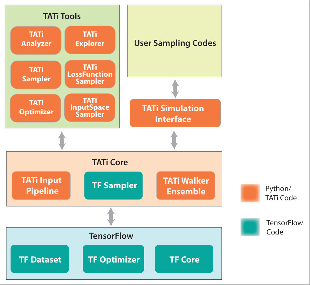 Figure 1
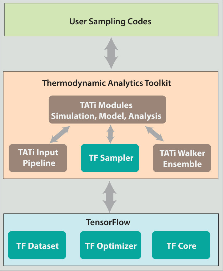 Figure 2
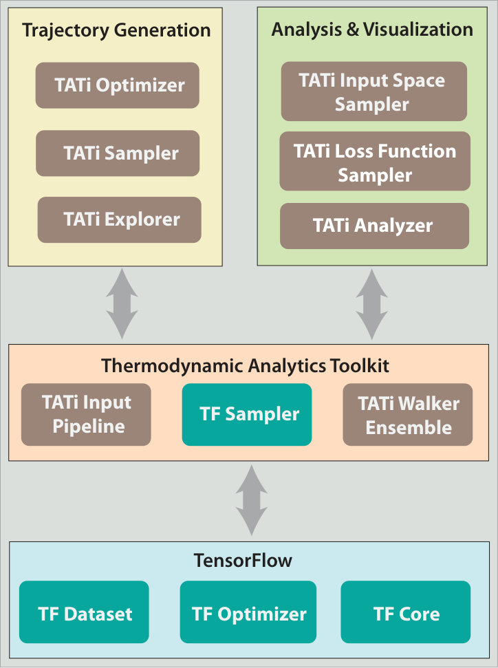 Figure 3
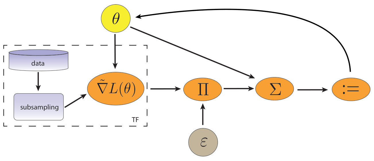 Figure 4
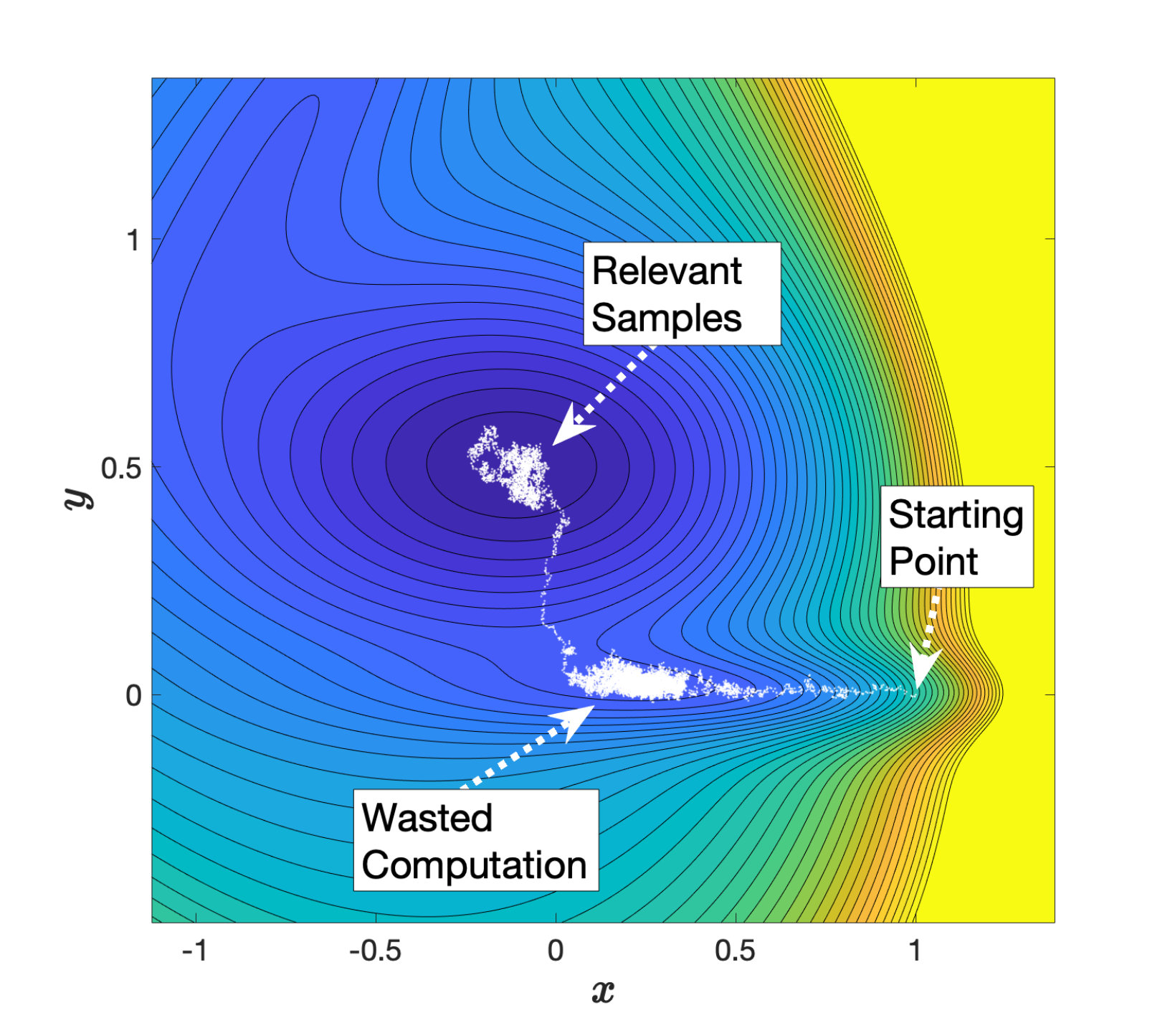 Figure 5
 Figure 6
 Figure 7
 Figure 8
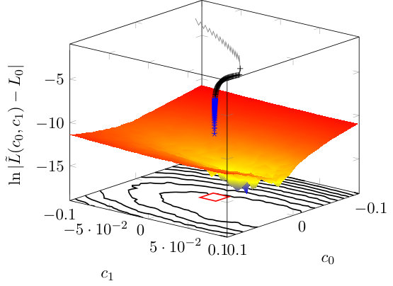 Figure 9
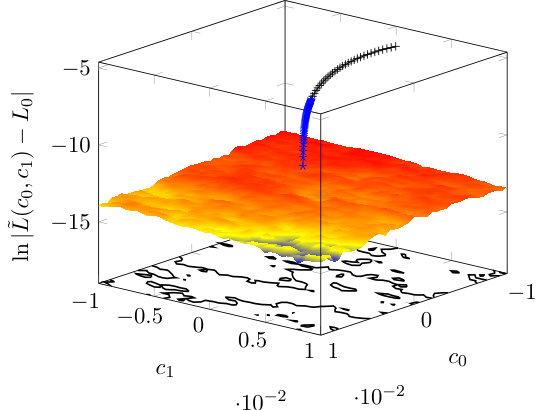 Figure 10
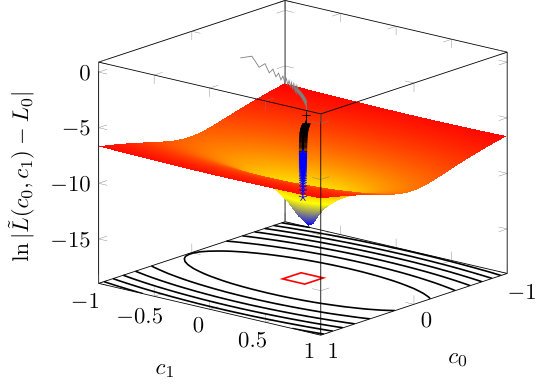 Figure 11
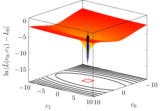 Figure 12
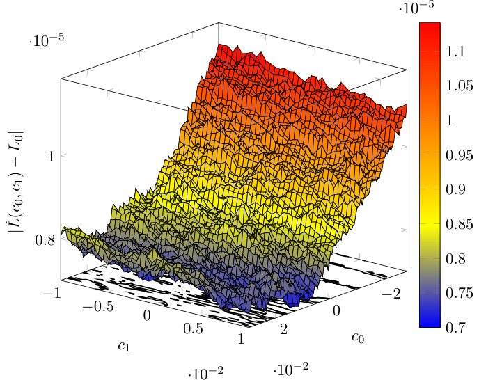 Figure 13
 Figure 14
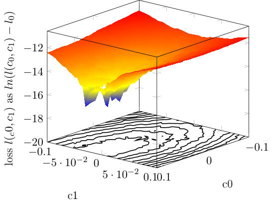 Figure 15
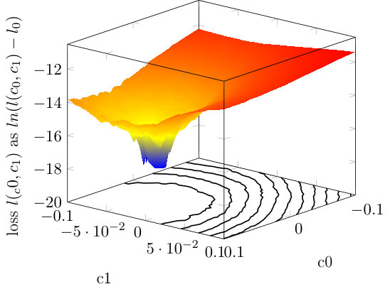 Figure 16
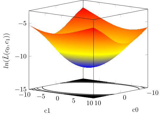 Figure 17
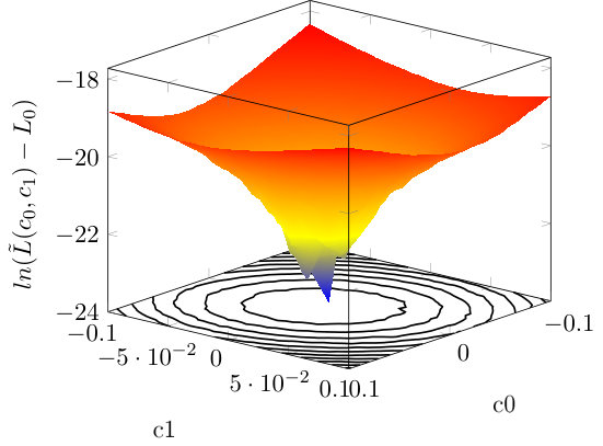 Figure 18
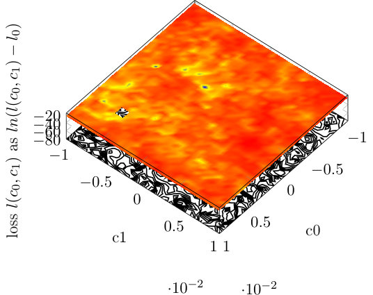 Figure 19
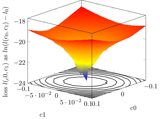 Figure 20
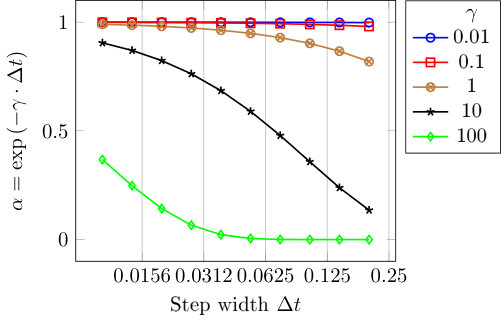 Figure 21
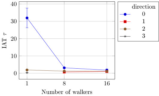 Figure 22
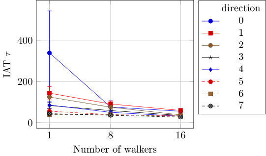 Figure 23
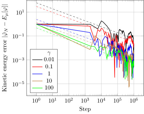 Figure 24
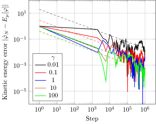 Figure 25
 Figure 26
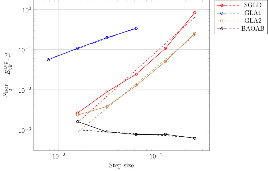 Figure 27
 Figure 28
 Figure 29
 Figure 30
 Figure 31
 Figure 32
 Figure 33
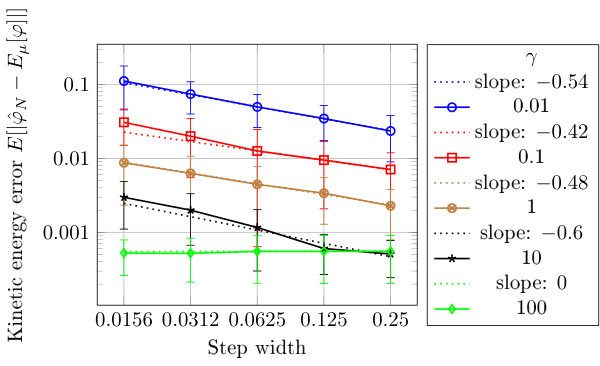 Figure 34
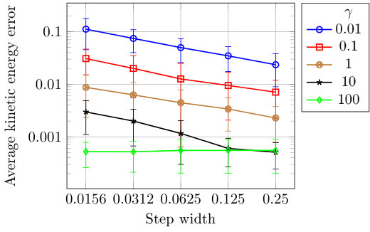 Figure 35
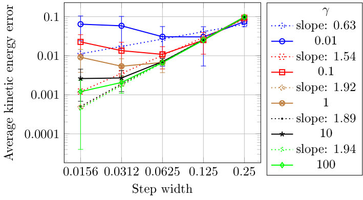 Figure 36
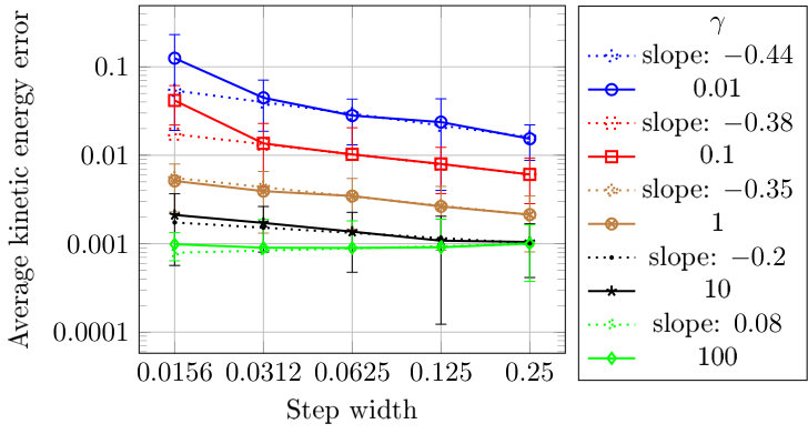 Figure 37
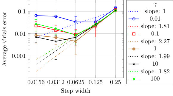 Figure 38
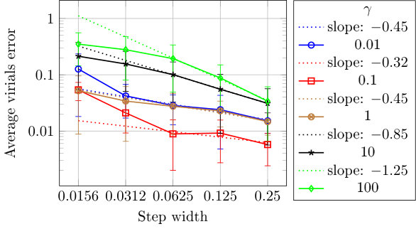 Figure 39
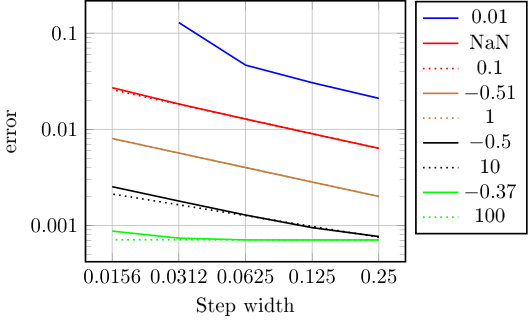 Figure 40
Peer Reviews
No public reviews on file for this paper yet. If you reviewed it on a platform where reviews are public (OpenReview, ICLR, NeurIPS, ICML), you can paste yours below so the community can read it here.
Videos
No videos yet. Explain this paper in a talk, walkthrough, or lecture? Add one.
Taxonomy
TopicsMachine Learning in Materials Science · Gaussian Processes and Bayesian Inference · Stochastic Gradient Optimization Techniques
TATi-Thermodynamic Analytics ToolkIt: TensorFlow-based software for posterior sampling in machine learning applications
Frederik Heber, Zofia Trstanova, Benedict Leimkuhler
Abstract
With the advent of GPU-assisted hardware and maturing high-efficiency software platforms such as TensorFlow and PyTorch, Bayesian posterior sampling for neural networks becomes plausible. In this article we discuss Bayesian parametrization in machine learning based on Markov Chain Monte Carlo methods, specifically discretized stochastic differential equations such as Langevin dynamics and extended system methods in which an ensemble of walkers is employed to enhance sampling. We provide a glimpse of the potential of the sampling-intensive approach by studying (and visualizing) the loss landscape of a neural network applied to the MNIST data set. Moreover, we investigate how the sampling efficiency itself can be significantly enhanced through an ensemble quasi-Newton preconditioning method. This article accompanies the release of a new TensorFlow software package, the Thermodynamic Analytics ToolkIt, which is used in the computational experiments.
1 Introduction
The fundamental role of neural networks (NNs) is readily apparent from their widespread use in machine learning in applications such as natural language processing ([72]), social network analysis ([26]), medical diagnosis ([7, 35]), vision systems ([65]), and robotic path planning ([44]). The greatest success of these models lies in their flexibility, their ability to represent complex, nonlinear relationships in high-dimensional data sets, and the availability of frameworks that allow NNs to be implemented on rapidly evolving GPU platforms ([40, 29]). The industrial appetite for deep learning has led to very rapid expansion of the subject in recent years, although, as pointed out by [19], at times the mathematical and theoretical understanding of these methods has been swept aside in the rush to advance the methodology.
The potential impact on society of machine learning algorithms demands that their exposition and use be subject to the highest standards of clarity, ease of interpretation, and uncertainty quantification. Typical NN training seeks to optimize the parameters of the network (biases and weights) under the constraint that the training data set is well approximated ([28, 23]). In the Bayesian setting, the parameters of a neural network are defined by the observations, but only in the probabilistic sense, thus specific parameter values are only realized as modes or means of the associated distribution, which can require substantial computation. Bayesian approaches based on exploration of the posterior probability distribution have been discussed throughout the development of neural networks ([54, 59, 31, 3]), and underpin much of the work in this field, but they are less commonly implemented in practice for “big data” applications due to legitimate concerns about efficiency ([71]). While the idea of sampling (or partially sampling) the posterior of large scale neural networks is not new, improvements in computers continually render this goal more plausible. For a recent discussion, see the PhD thesis of [22], which again champions the use of a (Bayesian) statistical framework, mentioning among other aims the prospect for meaningful uncertainty quantification in deep neural networks. Posterior sampling has the potential for broad impact in several research areas related to NN construction, including: (i) the relationship between network architecture and parameterization efficiency (Safran and Shamir [64], Livni et al. [53], Haeffele and Vidal [27], Soltanolkotabi et al. [68]), (ii) the visualization the loss manifold and the parameterization process (see Draxler et al. [17], Im et al. [34], Li et al. [52], Goodfellow et al. [23]), (iii) and the assessment of the generalization capability of networks (see Dinh et al. [16], Hochreiter and Schmidhuber [32], Kawaguchi et al. [37], Hoffer et al. [33]).
We have recently developed the \IfNextTokenThermodynamic Analytics ToolkIt (TATi)TATi, a python framework whose purpose is to facilitate the sampling of the posterior parameter distribution of automated machine learning systems with a balance of ease of use and computational efficiency, by leveraging highly optimised computational procedures within TensorFlow.111Installation of TATI is as simple as pip install tati from the unix command line; the software includes a readable user guide and programmer’s manual. Although still at an early stage in its development, this software package makes possible the exploration of sampling-based approaches in the high-dimensional setting. This article provides the motivation for TATi by illustrating that it facilitates analysis of the loss manifold in a way which would be impossible using standard optimization methods.
The standard approach to Bayesian sampling in high dimensions relies on Markov Chain Monte Carlo methods, but these can be difficult to scale to large system size. In the context of deep learning, we use the term large to refer both to large data set size (which translates into expensive likelihood computations) and to large numbers of parameters (usually the consequence of adopting a deep learning paradigm). We base our software on discretized stochastic differential equations which offer a reliable and accurate means of computing \IfNextTokenMarkov Chain Monte Carlo (MCMC)MCMC sampling paths while providing rigorous results with statistical error bounds ([48]). An underlying assumption in using software like this is that the exploration is limited to a bounded region of the parameter space by some structural features of the problem and/or its regularization. The methodology we describe could also be extended to include an explicit localization scheme to implement a quasi-stationary (spatially restricted) distribution [15], although we do not discuss this here.
As an indication of the possible scope for practical posterior sampling in large scale machine learning, we note that Markov Chain Monte Carlo methods like those implemented in \IfNextTokenTATiTATi have been successfully deployed in the more mature setting of very large scale molecular simulations in computational sciences for applications in physics, chemistry, material science and biology, with variables numbering in the millions or even billions ([39, 73, 36]). The goal in molecular dynamics is similarly the sampling of a target probability distribution, although the distribution typically arises from semi-empirical modelling of interactions among atoms of the substances of interest. The scientific communities in molecular sciences are developing highly efficient “enhanced sampling” procedures to tackle the computational difficulties of large scale sampling (see the surveys ([21, 4]) for some examples of the wide variety of methods being used in biomolecular applications). In analogy with molecular dynamics, the focus on posterior sampling makes possible the elucidation of reduced descriptions of neural networks through concepts such as free energy calculation ([51]) and transition path sampling ([6]). Although we reserve detailed study of these ideas for future work, the fundamental tool in their construction and practical implementation is the ability to compute sample sequences efficiently and reliably using \IfNextTokenMCMCMCMC paths. Further potential benefits of the posterior sampling approach lie in the fact that it offers a means of high-dimensional uncertainty quantification through standard statistical methodology ([67, 22]).
We favor schemes based on underdamped Langevin dynamics (with canonical momentum variables). Such methods have excellent properties in terms of accuracy of statistical averages and convergence rates ([48, 51]). A variety of other methods are available which are also based on second order dynamics ([11, 61, 66, 57]). One of the purposes of the TATi software is to provide a relatively simple mechanism for the implementation and evaluation of sampling strategies of statistical physics in machine learning applications. 222 While TensorFlow’s graph programming structure is well explained and motivated by its developers and provides efficient execution on GPUs, it is not straightforward for numerical analysts, statisticians and statistical physicists to modify in order to test their methods. \IfNextTokenTATiTATi therefore uses a simplified interface structure that allows algorithms to be coded directly in pure Python and then linked to TensorFlow for efficient calculation of gradients for arbitrary TensorFlow models. As a consequence, building and testing a new sampling scheme in \IfNextTokenTATiTATi requires little knowledge of the underpinnings of TensorFlow.
Another goal we have had in mind in this study is to gain insight into the loss landscape (given by the log of the posterior density) so as to better understand its structure vis a vis the performance of parameterization algorithms. The loss is not convex in general ([43, sect. 4]), and its corrugated (“metastable”) structure has been compared to models of spin-glasses ([13]): there is a band of minima close to the global minimum as lower bound and whose multitude diminishes exponentially for larger loss values. The availability of an efficient sampling scheme gives a means of better understanding the loss landscape and its relation to the network (and properties of the data set). We illustrate some of the potential for such studies in Section 3 of this article, where we examine the loss landscape of an MNIST classification problem.
Finally, we note that the statistical perspective underpins many optimization schemes in current use in machine learning, such as the \IfNextTokenStochastic Gradient Descent (SGD)SGD method. The stochasticity enters into this method through the subsampling of the dataset at every iteration of the optimization algorithm, due to ‘minibatching’. Several stochastic optimisation methods have been proposed which aim to improve the computational efficiency or reduce generalisation error, e. g., RMSprop ([30]), AdaGrad ([18]), Adam ([38]), entropy-SGD ([10]). \IfNextTokenStochastic Gradient Langevin Dynamics (SGLD)SGLD ([71]), and these, similarly, can be given a statistical (sampling) interpretation. Indeed, when its stepsize is held fixed and under simplifying assumptions on the character of the gradient noise, it can be viewed as a first-order discretization of overdamped Langevin dynamics. We discuss \IfNextTokenSGDSGD and \IfNextTokenSGLDSGLD in Sec 2, in order to motivate SDE sampling methods.
The remainder of this paper is structured as follows: Section 2 provides an overview of \IfNextTokenMCMCMCMC, Langevin dynamics schemes and other sampling strategies and the concepts from numerical error analysis that underpin our approach. We also outline there the Ensemble Quasi-Newton method ([49]). Subsequently, in Section 3, we discuss the accuracy of various schemes as well as their convergence behavior in the context of neural network posterior sampling. We also elaborate on how the approach we describe can be used to handle moderate-dimensional sampling on the MNIST dataset. The last part of this section consists of a demonstration of the convergence acceleration of the EQN sampler in the MNIST application. The numerical results presented in the paper represent a proof-of-concept for the utility of the posterior sampling paradigm and the TATi software which implements it.
2 Markov Chain Monte Carlo methods and stochastic differential equations
In this section, we provide a brief introduction to the \IfNextTokenMCMCMCMC methods we have used for sampling high dimensional distributions. These methods include schemes based on discretization of stochastic differential equations, especially Langevin dynamics. We discuss in some detail the construction of numerical schemes in order to control the finite time stepsize bias. Moreover, we also describe an ensemble quasi-Newton method implemented in TATi that adaptively rescales the dynamics to enhance sampling of poorly conditioned target posteriors.
Assume that we are given a dataset comprising inputs and outputs of an unknown functional relationship. We also assume we are given a neural network defined by a vector of parameters which acts on an input to produce output . The goal of training the network is then typically formulated as solving an optimization problem over the parameters given the dataset:
[TABLE]
where the function is the total loss function associated to the dataset , defined by
[TABLE]
The loss function depends on the metric choice, for example the squared error, logarithmic loss, cross entropy loss, etc ([63]). The total loss is in general not a convex function of the parameters even though may be convex as a function of . In general the loss landscape is rough there are likely to be many local minima and flattened intermediate states in the loss manifold , as well as many saddles, see [1, 13].
The parametrization procedure is based on optimization algorithms, which generate a sequence of parameter vectors , converging to a (local) minimizer of (1) as . The basic optimization algorithm is the \IfNextTokenGradient Descent (GD)GD, which uses the negative gradient to update the parameter values, i. e.,
[TABLE]
where is the stepsize (or learning rate), which is either constant or may be varied during the computation. \IfNextTokenGDGD converges for a convex function and for a smooth non-convex total loss function it converges to the nearest local minimum ([60]).
Gradient calculations are the primary computational burden when training neural networks, i. e., the computational cost of a gradient can be taken as a reasonable measure of computational work. As the total loss implicitly depends on the whole dataset, one natural idea that reduces the computational cost is to exploit the redundancy in the dataset by estimating the gradient of the average loss from a subset of the data, that is, to replace the gradient in each parameterization step by the approximation
[TABLE]
Where represents a randomized data subset (re-randomized throughout the training process) of dimension , this method, which has many variants, is referred to as \IfNextTokenSGDSGD.
We are interested in the Bayesian inference formulation, where is the parameter vector and we wish to sample from the posterior distribution of the parameters given a dataset of size ,
[TABLE]
with prior probability density , and likelihood .
\IfNextToken
Stochastic Gradient Langevin Dynamics (SGLD)Stochastic Gradient Langevin Dynamics (SGLD) ([71]) generates a step based on a subset of the data and injects additional noise. The additive noise creates a controllable stochastic model with known ergodic properties and it improves the numerical stability and convergence properties of the training algorithm. For additional discussion of these points see [50], where small injected noise has been shown to substantially accelerate and improve robustness of the training process for neural network models.
The \IfNextTokenSGLDSGLD parameter update is using a sequence of stepsizes and reads
[TABLE]
with
[TABLE]
where is a constant (in physics, it would be associated with reciprocal temperature) and again is a random subset of indices of size . The original algorithm uses a diminishing stepsize sequence, however, [70] showed that fixing the stepsize has the same efficiency, up to a constant.
Under the assumption that the gradient noise is uncorrelated and identically distributed from step to step, it is easy to demonstrate that \IfNextTokenSGLDSGLD with fixed stepsize is an Euler-Maruyama (first order) discretization of overdamped Langevin dynamics ([71]):
[TABLE]
This creates a natural starting point for our approach: we simply change the perspective to focus on the sampling of the posterior distribution, rather than the identification of its mode.
In case a full gradient is used, dynamics (5) preserves the Boltzmann distribution with measure proportional to an exponential function of the negative loss:
[TABLE]
Given a generic process providing samples asymptotically distributed with respect to a defined target measure , it is possible to use sampling paths to estimate integrals with respect to . Define the finite time average of a function by
[TABLE]
For an ergodic process, we have
[TABLE]
The convergence rate of the limit above is given by the \IfNextTokenCentral Limit Theorem (CLT)CLT. Given a generic process generating samples from a target distribution with density , the variance of an observable behaves, asymptotically for large , as
[TABLE]
where is the integrated autocorrelation time, see Goodman and Weare [25, sect. 3]. can be viewed as a measure of the redundancy of the sampled values or the number of steps until the sampled values of decorrelate, thus is optimal, i. e., immediately stepping from one independent state to the next. The \IfNextTokenIntegrated Autocorrelation Time (IAT)IAT can also be calculated as
[TABLE]
where the covariance is averaged over the initial condition.
In practice, the process of discretization of the SDE introduces asymptotic bias, which is controlled by the stepsize, however it is nonetheless possible and useful to compute the IAT in such a case to describe the convergence to the asymptotically perturbed equilibrium distribution.
Langevin Dynamics.
Sampling from (6) is one of the main challenges of computational statistical physics. There are three popular alternative approaches to sample from (6): discretization of continuous stochastic differential equations (SDEs), Metropolis-Hastings based algorithms and deterministic dynamics, as well as combinations among the three groups.
Langevin dynamics is an extended version of (5):
[TABLE]
where is the momentum variable and is the friction. The fluctuation-dissipation relation ensures that the extended (canonical) distribution with density
[TABLE]
is preserved; the target distribution is recovered by marginalization.
Whereas the momentum is a physical variable in statistical mechanics, it is introduced as an artificial auxiliary variable in the machine learning application. in (9) is a positive definite mass matrix, which can in many cases be taken to the identity matrix.
The discretization of stochastic dynamics introduces bias in the invariant distribution (see below, for discussion). Although the bias can be removed through the incorporation of a \IfNextTokenMetropolis-Hastings (MH)MH step, such methods do not always scale well with the dimension [5, 62]; and the \IfNextTokenMHMH test is often neglected in practice. For example the “unadjusted Langevin algorithm” of [20] tolerates the presence of small stepsize-dependent bias, in order to obtain faster convergence (reduced asymptotic variance or lower integrated autocorrelation time for observables of interest) and better overall efficiency.
Systematic design of schemes.
The mathematical foundation for the construction of discretization schemes for (9) by splitting of the generator of the dynamics is now well understood ([48]). Although different choices can be made, the usual starting point is an additive decomposition of the generator of dynamics (9) into three operators , where
[TABLE]
The main idea is that each of these sub-dynamics can be resolved exactly in the weak (distributional) sense. Note that the (“O” step) dynamics
[TABLE]
has an analytical solution
[TABLE]
A Lie-Trotter splitting of the elementary evolution generated by and provides six possible first-order splitting schemes of the general form
[TABLE]
with all possible permutations of , and second-order splitting schemes are then obtained by a Strang splitting of the elementary evolutions generated by and .
Using the notation for the three operators of the sub-dynamics (10), we define the following updates which will be combined in the full scheme for the discretization of the Langevin dynamics with stepsize :
[TABLE]
with and . A numerical methods is easily specified by a string such as ‘ABO’. This is an instance of the Geometric Langevin Algorithm ([9]). We also consider symmetric compositions of several basic steps. The ‘BAOAB’ scheme is in this notation . This method can be written out in detail as a step from to as follows:
[TABLE]
Given the sequence of samples determined using such a method, we can approximate expected values of a function of and using the standard estimator based on trajectory averages
[TABLE]
It can be shown in certain cases that these discrete averages converge to an ensemble average,
[TABLE]
where represents the stationary density of the (biased) discrete process. Under specific assumptions on the splitting scheme ([48]), an expansion may be made in the time stepsize of the invariant measure of the splitting scheme which guarantees that the error in an ergodic approximation of an observable average is bounded relative to , where depends on the detailed structure of the numerical method. Thus
[TABLE]
Schemes such as “ABO” can be shown to be first order (), whereas BAOAB and ABOBA are second order. Delicate cancellations imply that BAOAB can exhibit an unexpected fourth order of accuracy in the “high friction” limit () when the target is sampling of configurational (-dependent) quantities. The latter method also has remarkable features with respect configurational averages in harmonic systems and near-harmonic systems [47].
All explicit Langevin integrators are subject to stability restrictions which require that the product of stepsize and the frequency of the fastest oscillatory mode is bounded.
Hybrid Monte Carlo
Hybrid Monte-Carlo, also called Hamiltonian Monte Carlo, is a \IfNextTokenMCMCMCMC method based on the \IfNextTokenMetropolis-HastingsMetropolis-Hastings algorithm that allows one to sample directly from the target distribution . Starting from an initial position , the momenta are re-sampled from and a proposal is obtained by evaluating times the Verlet method, i.e., . The proposal is then accepted with a probability given by the Metropolis ratio:
[TABLE]
where the energy is given by . In case the proposal is rejected, the state is reset to the starting point . The number of steps is often randomized. The parameterization of this method depends on the trade-off between the larger time stepsizes and the number of steps , implying higher rejection rates for the proposals and smaller stepsizes leading to potentially slow exploration of the parameter space. To our knowledge, there is currently no extension of HMC to the case of noisy gradients which retains the exact sampling property.
Multiple walkers: the ensemble quasi-Newton method
We next comment on more exotic sampling schemes which can give higher sampling efficiency. One such scheme is the preconditioned method developed in [49] which we refer to as the “\IfNextTokenensemble quasi-Newtonensemble quasi-Newton” (EQN) method. The idea of this scheme is easily motivated by reference to a simple harmonic model problem in two space dimensions in which the stiffness (or frequency of oscillation) is very high in one direction and not in the other. The stepsize for stable simulation using a Langevin dynamics strategy will be determined by the high frequency term meaning that the exploration rate suffers in the slowest direction. Effectively the integrated autocorrelation time in the “slow” direction is large compared to the timestep of dynamics.
In the harmonic case it is easy to rescale the dynamical system in such a way that sampling proceeds rapidly. In the more complicated setting of nonlinear systems in multiple dimensions, the idea that a few directions may restrict the progress of the sampling still has merit, but we no longer have direct access to the underpinning frequencies. The idea is to determine this rescaling adaptively and dynamically during simulation. There are several ways to do this in practice (see [42] for an early related work on using Hessian information to speed up convergence of \IfNextTokenGDGD).
As a simple illustration consider a Gausssian mixture model as shown in Figure 1. Here, a poor choice of initial condition has led to a naive sampling path (here generated using Euler-Maruyama and shown in white) getting stuck for a long time in a poorly scaled basin. Eventually the sampler proceeds to the deeper (and more relevant) basin, but not before a great deal of useless computational effort has been expended. Note that the stepsize threshold for stable integration of the SDE is inversely proportional to the frequency of the largest normal mode of oscillation in the local basin, thus it is not possible to simply ’step over’ the irrelevant intermediate region by using large stepsizes. This process mimics the behavior of many optimization schemes as well.
In the paper of [49] modified dynamics (”Ensemble Quasi-Newton” or EQN for short) is based on construction of the covariance matrix of the walker collection. This matrix is computed during simulation to determine the appropriate dynamical rescaling. The implementation is somewhat involved, thus making it an excellent demonstration of \IfNextTokenTATiTATi’s versatility and robustness.
We next briefly describe the EQN scheme; for more detail, the reader is referred to [49] (and, in particular, the Python code referenced within it). Suppose we have walkers (replicas). Denote by the position vector of the th walker and by the corresponding momentum vector, each of which is a vector in , where is the number of parameters of the network. We assume that the mass matrix of the underlying system is the identity matrix, for simplicity. The equations of motion for the th walker then take the form
[TABLE]
Here has the previous interpretation of a Wiener increment and is the tensor divergence. The matrix estimates the matrix square root of the covariance matrix which depends on the locations of all the walkers.
Under discretization, we compute steps in configurations and momenta at iteration step with walker index . We use a variant of the BAOAB discretization applied to walker :
[TABLE]
As in the code of [49], we make the calculation in (18b) explicit by updating only infrequently, typically every steps, and we define by
[TABLE]
In the above, the matrix square root is understood in the sense of a Cholesky factorization, is a covariance blending constant, and is the set of all walker positions at timestep , excluding those of walker itself. Note that for moderate the choice (19) is always positive definite even if . However, with (19) the affine invariance property, an elegant feature of the original system, no longer strictly holds. Nonetheless, the simplified method has been shown to work very well in practice [49, sect. 4].
3 Numerical Experiments
In this section, we first look at the convergence rates and accuracy of the samplers described previously for the simplified case of a harmonic oscillator, comparing them with analytically known rates. Next we turn to a very simple clustering problem to further explore the error (bias) introduced by SDE schemes; we show that a particular discretization (“BAOAB”) of underdamped Langevin dynamics offers extraordinarily high accuracy compared to several alternative, mimicing observations about this scheme in the molecular dynamics setting. Subsequently, we use the MNIST dataset on a single-layer perceptron to illustrate an enhanced loss landscape visualization technique that obtains its projection directions from sampling trajectories. Finally, we present results on the \IfNextTokenensemble quasi-Newton (EQN)EQN method described in Section 2 for a Gaussian model and for a single layer perceptron applied to the MNIST dataset.
3.1 Sampler Properties and Error Analysis
In this error analysis, we explore a state with position and momentum of a single degree of freedom. The kinetic energy is defined as , where we have set the mass matrix to unity. Its asymptotic value in the canonical distribution is given by the number of parameters and the (inverse) temperature as [46, sect. 6.1.5]. The virial is defined as , where is the derivative of the loss function with respect to the parameter . Its asymptotic value is two times that of the kinetic energy, as a consequence of the virial theorem. For this theorem to hold we need a potential that is unbounded from above and grows sufficiently rapidly at infinity, see appendix A.1 for a derivation.
Averages of the kinetic energy or of the virial are examples of time integrals of (7) that can be used to assess the accuracy of the chosen dynamics and discretization, since their asymptotic values are known. As we are interested in discretized integrals over finite number of time steps, which are accessible in numerical computations in the absence of analytical solutions, we look at estimators (14) of the following form
[TABLE]
The total error with respect to the expected value for the invariant probability measure decomposes as
[TABLE]
i.e. it is a combination of the discretization error, from the finite step size when discretizing the dynamics (9), and the sampling error that results from the inability to sample over an infinite time or to generate an infinite number of steps. The first source is also sometimes referred to as the perfect sampling bias, emphasizing its presence even in the limit of infinitely many samples.
In the extreme case of a vanishing gradient, only the sampling error is present. This error will decay so that its variance is proportional to . A more interesting case is that of a “harmonic potential” , in which case the truncation error is nontrivial.
3.1.1 Truncation Error for Harmonic Potential
We have contributions to the total error (20) from both the sampling error and the discretization error. We will see that the latter may dominate when the scale of the potential and therefore the average gradients are sufficiently large. We concentrate here on the empirical results; refer to Leimkuhler and Matthews [46, sect. 7.4] for a general discussion of harmonic problems in the context of Langevin dynamics. We use a single-layer perceptron with a single input node and a single output node with linear activation and zero bias, i. e. . We use the mean squared loss function. Then, such a harmonic potential can be easily introduced by a dataset with the square root of the prefactor as its single feature and a zero label, i. e. the only dataset item is . We use three different factors . Moreover, we use the following sets of parameters for , , and . Here, we employ BAOAB as the sampler, again with sampling steps.
Examining Figure 2(a) where we use a small prefactor , we notice that the error decreases with increasing step size because becomes smaller and therefore we obtain more random walk-like behavior. However, it does not entirely depend on , but also to some extent on the step size . For the highest value of we again have a flat line due to the lower bound enforced by the \IfNextTokenCLTCLT.
In Figure 2(b) with a large prefactor for large step sizes all of the curves coincide regardless of and the behavior has reversed: now the error becomes smaller for smaller step sizes. Naturally, the reason for this change is the discretization error that arises because of substantial non-zero gradients, and that the error depends on the step size . Measuring the slope in the domain where all curves overlap for , we obtain values of up to , i. e. second order convergence in the discretization error as expected from BAOAB. In place of the prefactor we could also have varied the inverse temperature to the same effect that only depends on the scale of the noise relative to the scale of the gradients.
Using a higher-order sampler allows for a smaller error at a given step size or to use larger step sizes (and therefore sample more space) for a given error threshold. Note that the step size is bounded from above by a stability threshold. The benefit of the trade-off between accuracy and computational effort is limited however, and it is likely that very high order schemes (beyond the second order splittings discussed here) are not efficacious in TATi, in keeping with previous studies in molecular dynamics ([47]).
For comparison, we also look at the average virials in Figure 3.1.1. However, they depend only on the position and not on momentum. Note that the BAOAB scheme has nil perfect sampling bias for purely configurational quantities such as virials. Here, we are instead using the \IfNextTokenGeometric Langevin Algorithm (GLA)GLA 2nd order sampler but keep all the other aspects of the method unchanged.
The reference list from the paper itself. Each links out to its DOI / PubMed record.
- 1Baldi and Hornik [1989] P. Baldi and K. Hornik. Neural networks and principal component analysis: Learning from examples without local minima. Neural Networks , 2(1):53–58, 1989.
- 2Ballard et al. [2017] A.J. Ballard, R. Das, S. Martiniani, D. Mehta, L. Sagun, J.D. Stevenson, and D.J. Wales. Energy landscapes for machine learning. Phys. Chem. Chem. Phys. , 19:12585–12603, 2017.
- 3Barber and Bishop [1998] D. Barber and C. M. Bishop. Ensemble learning in bayesian neural networks. Neural Networks and Machine Learning , 168:215–238, 1998.
- 4Bernardi et al. [2015] R. Bernardi, M. Melo, and K. Schulten. Enhanced sampling techniques in molecular dynamics simulations of biological systems. Biochimica et Biophysica Acta (BBA) - General Subjects , 1850(5):872 – 877, 2015.
- 5Beskos and Stuart [2009] A. Beskos and A. Stuart. Computational complexity of Metropolis-Hastings methods in high dimensions. In Pierre L’ Ecuyer and Art B. Owen, editors, Monte Carlo and Quasi-Monte Carlo Methods 2008 , pages 61–71. Springer, 2009.
- 6Bolhuis et al. [2002] P.G. Bolhuis, D. Chandler, C. Dellago, and P.L. Geissler. Transition path sampling: Throwing ropes over rough mountain passes, in the dark. Annual Review of Physical Chemistry , 53(1):291–318, 2002.
- 7Bone et al. [2015] D. Bone, M. Goodwin, M. Black, C.-C. Lee, K. Audhkhasi, and S. Narayanan. Applying machine learning to facilitate autism diagnostics: pitfalls and promises. J. Autism Dev. Disord. , 45:1121–1136, 2015.
- 8Bottou et al. [2018] L. Bottou, F. Curtis, and J. Nocedal. Optimization methods for large-scale machine learning. SIAM Review , 60(2):223–311, 2018.