Spectral enclosures for non-self-adjoint discrete Schr\"odinger operators
Orif O. Ibrogimov, Franti\v{s}ek \v{S}tampach

TL;DR
This paper investigates the eigenvalue locations of one-dimensional discrete Schrödinger operators with complex potentials in various ℓ^p spaces, establishing optimal bounds for ℓ^1 and new bounds for p>1 using the Birman-Schwinger method.
Contribution
It provides the first optimal eigenvalue bounds for ℓ^1 potentials and introduces new spectral bounds for ℓ^p potentials with p>1 in discrete Schrödinger operators.
Findings
Optimal eigenvalue bounds for ℓ^1 potentials.
New spectral bounds for p>1 potentials.
Method relies on Birman-Schwinger principle and norm estimations.
Abstract
We study location of eigenvalues of one-dimensional discrete Schr\"odinger operators with complex -potentials for . In the case of -potentials, the derived bound is shown to be optimal. For , two different spectral bounds are obtained. The method relies on the Birman-Schwinger principle and various techniques for estimations of the norm of the Birman-Schwinger operator.
Click any figure to enlarge with its caption.
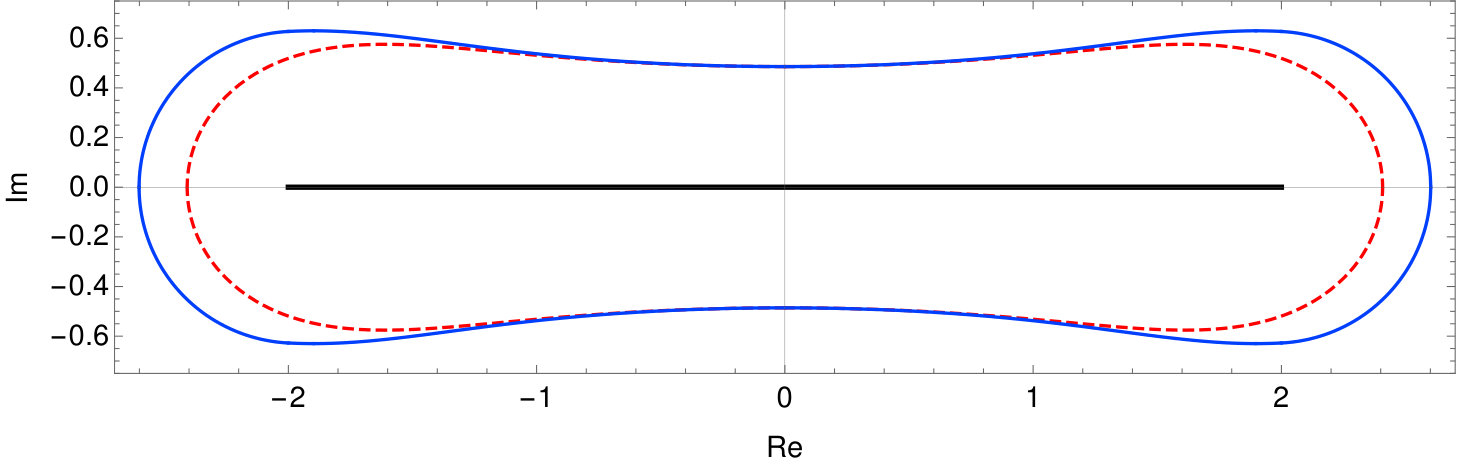 Figure 1
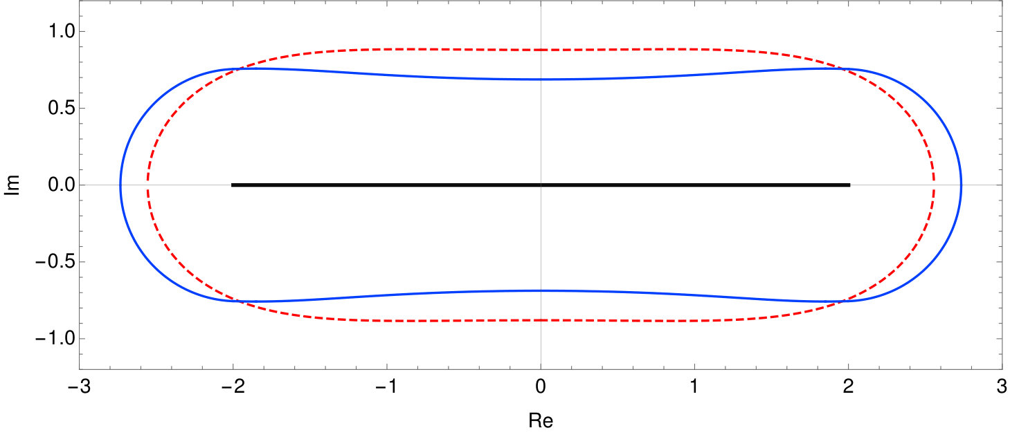 Figure 2
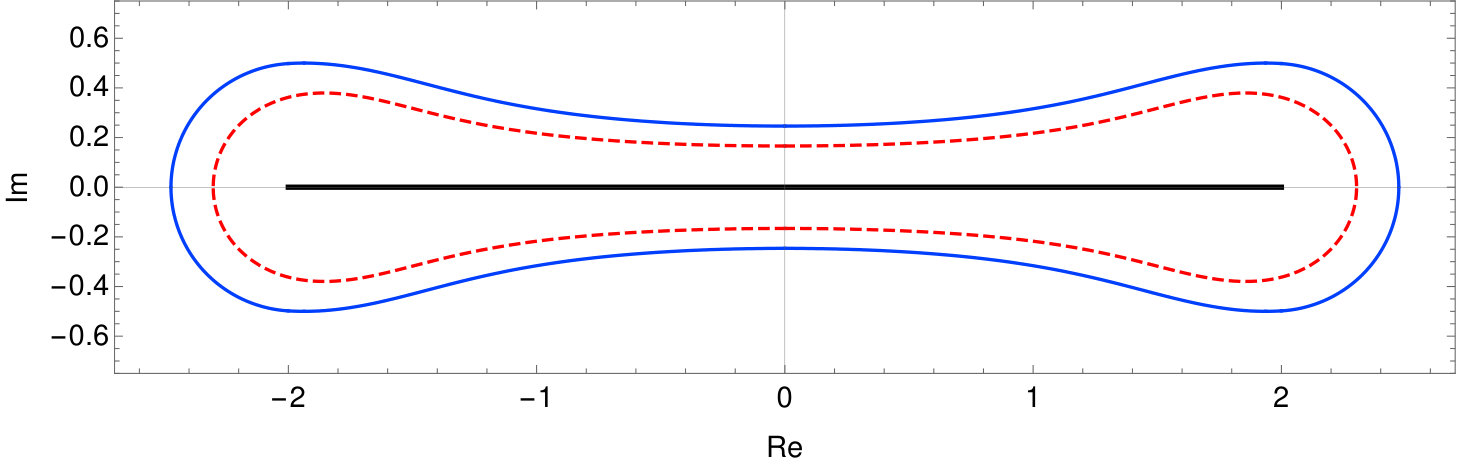 Figure 3
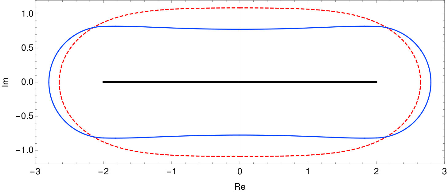 Figure 4
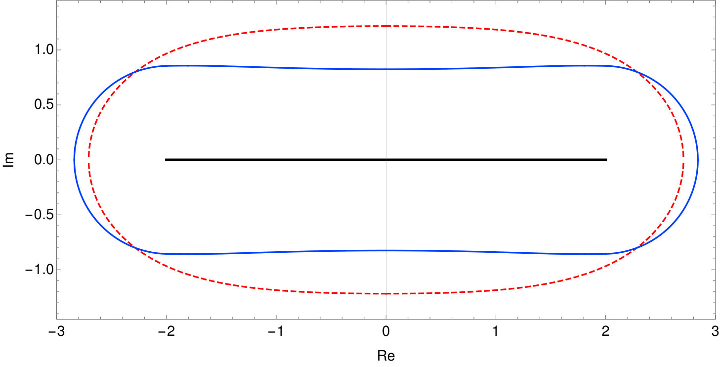 Figure 5
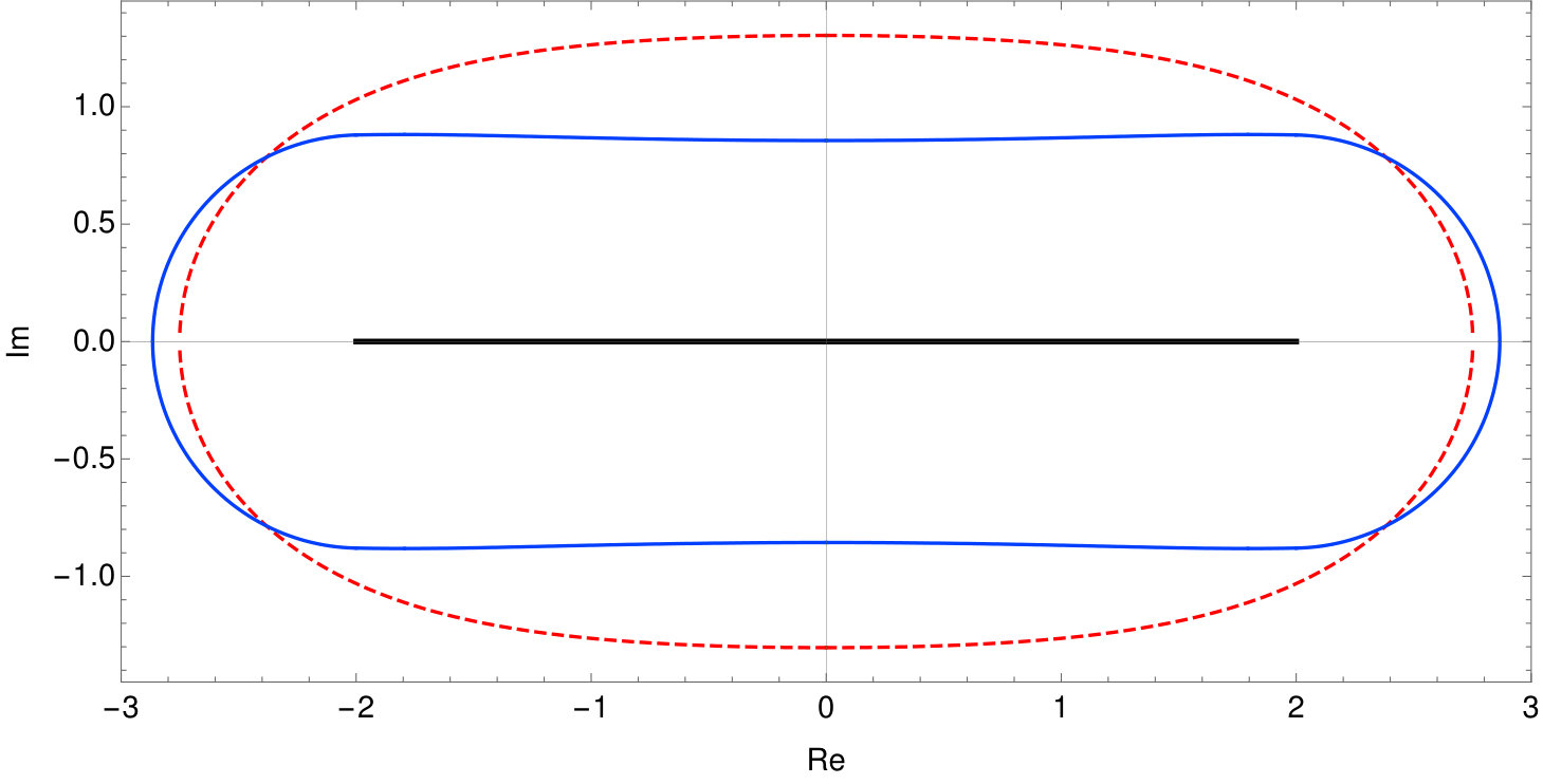 Figure 6
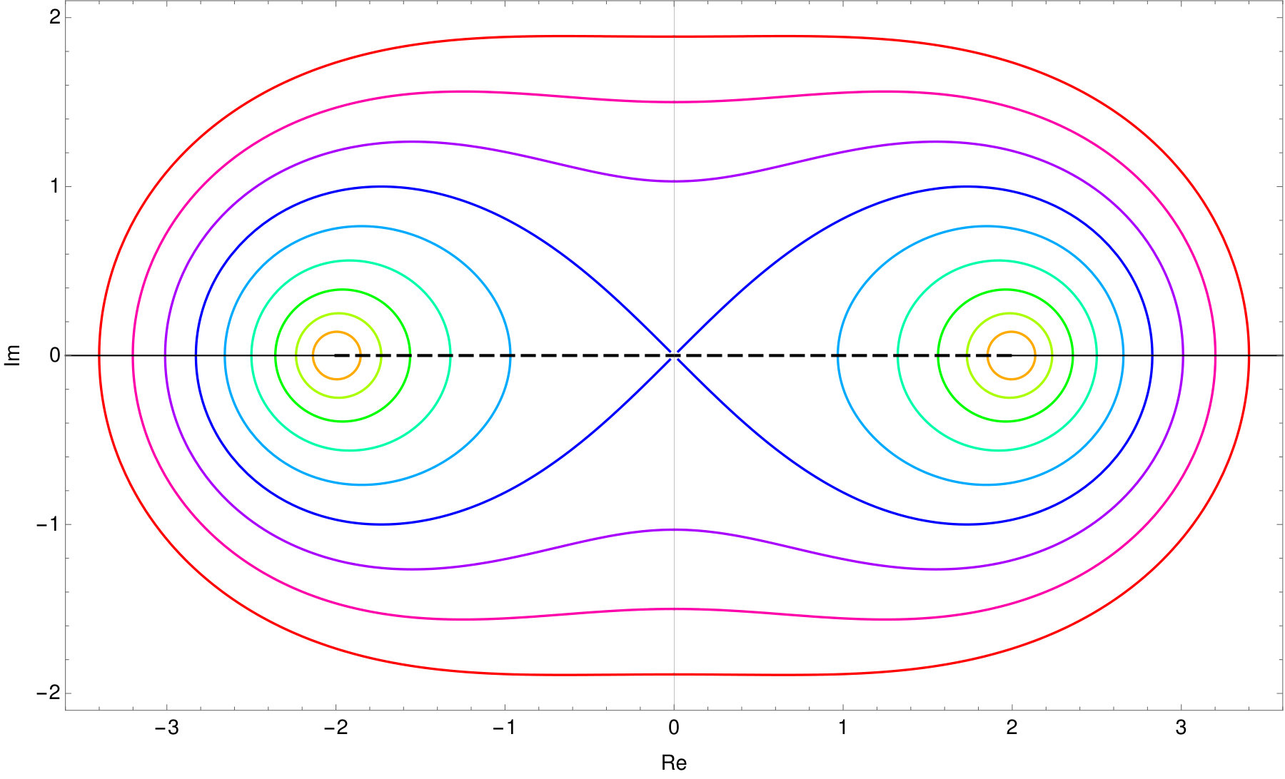 Figure 7
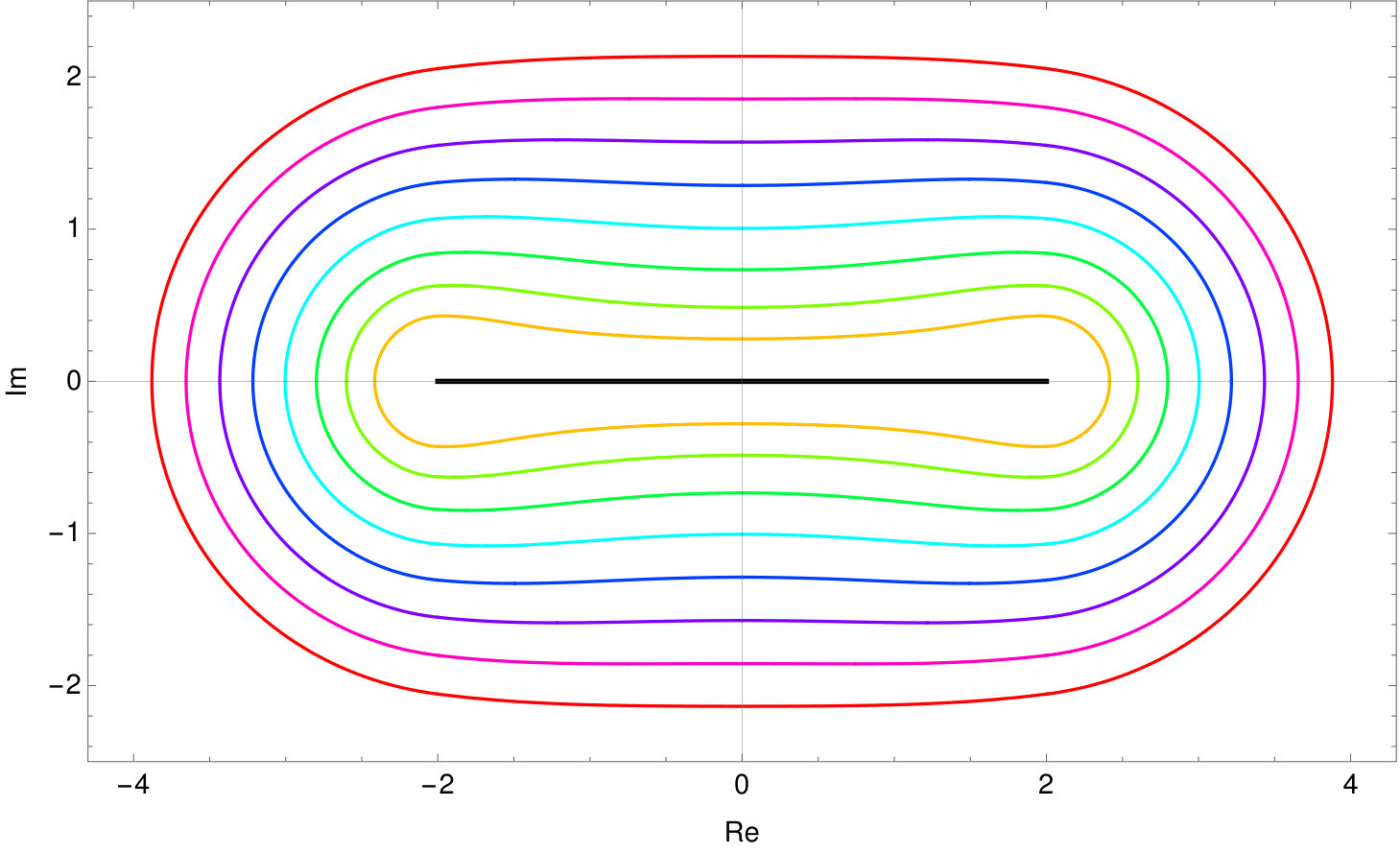 Figure 8
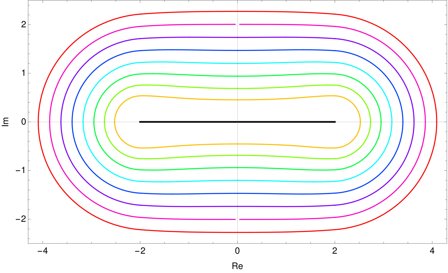 Figure 9
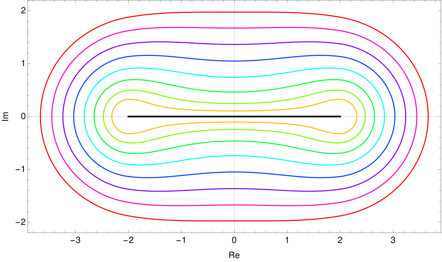 Figure 10
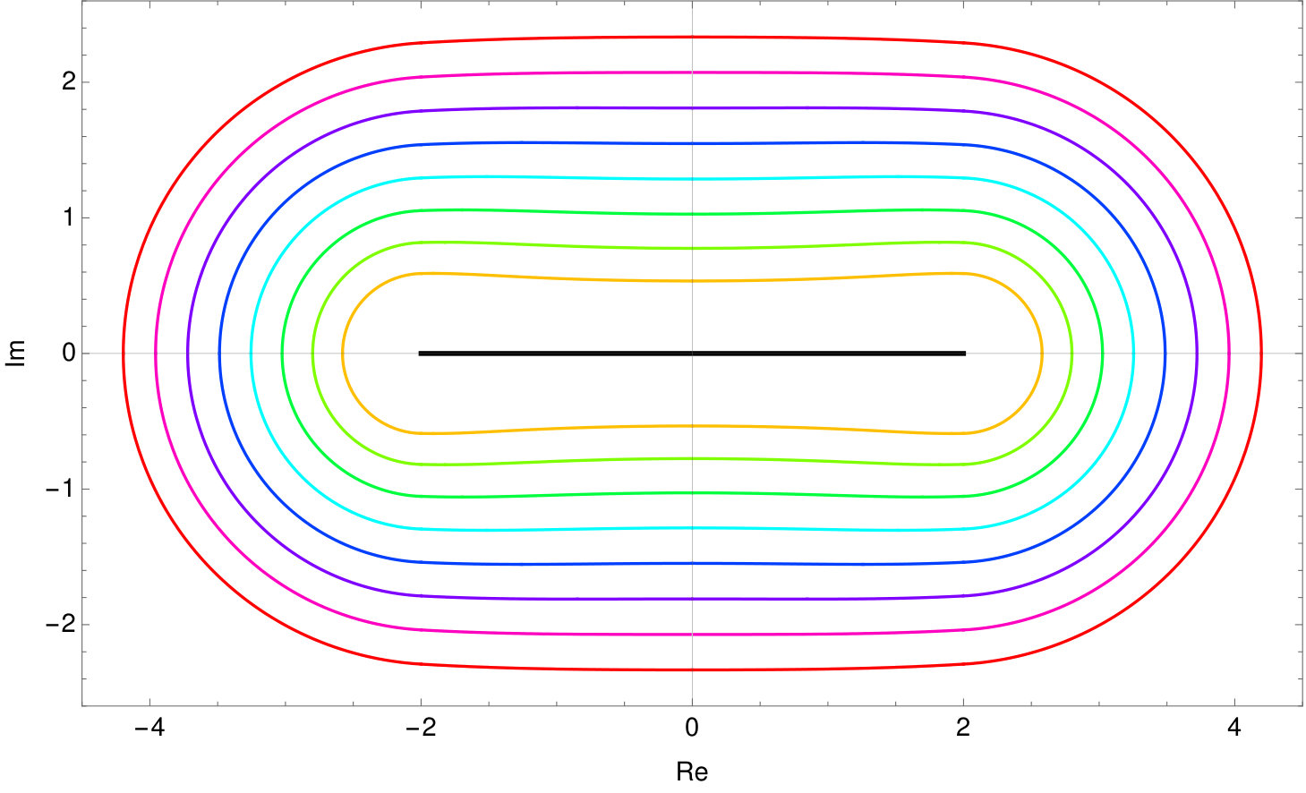 Figure 11
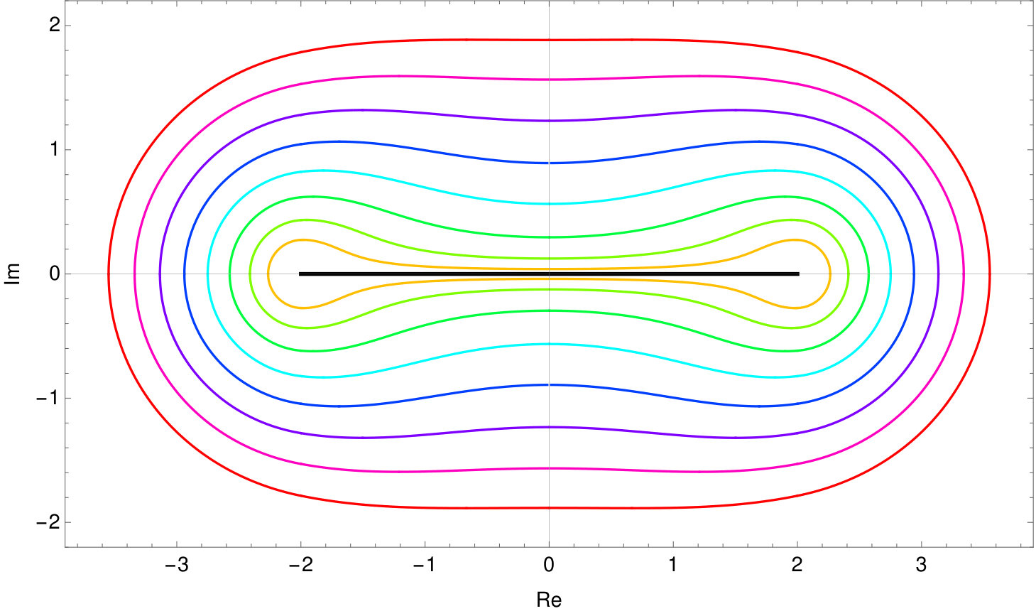 Figure 12
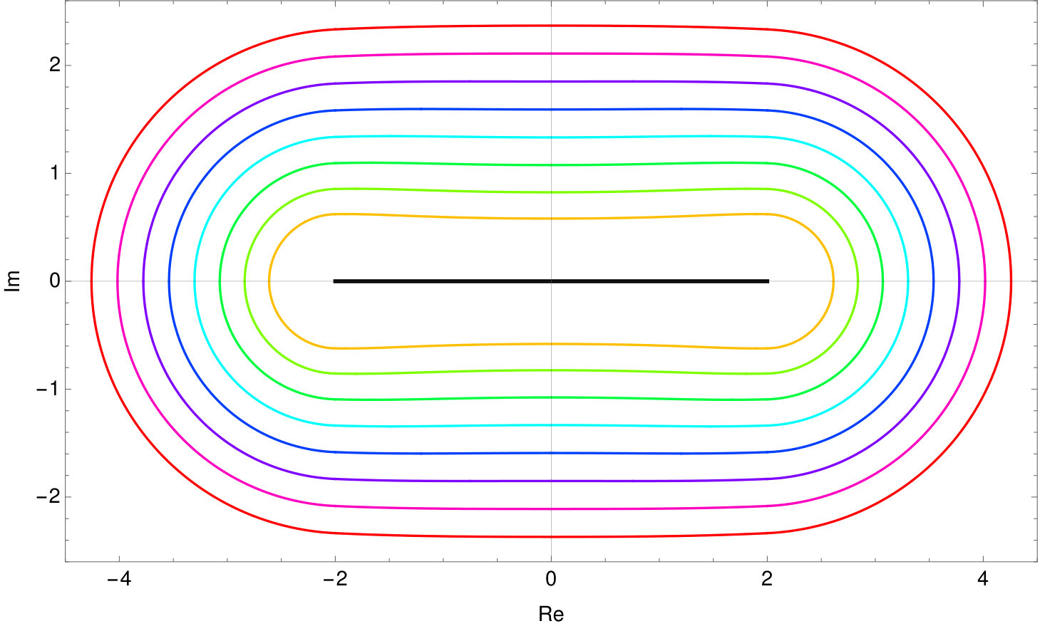 Figure 13
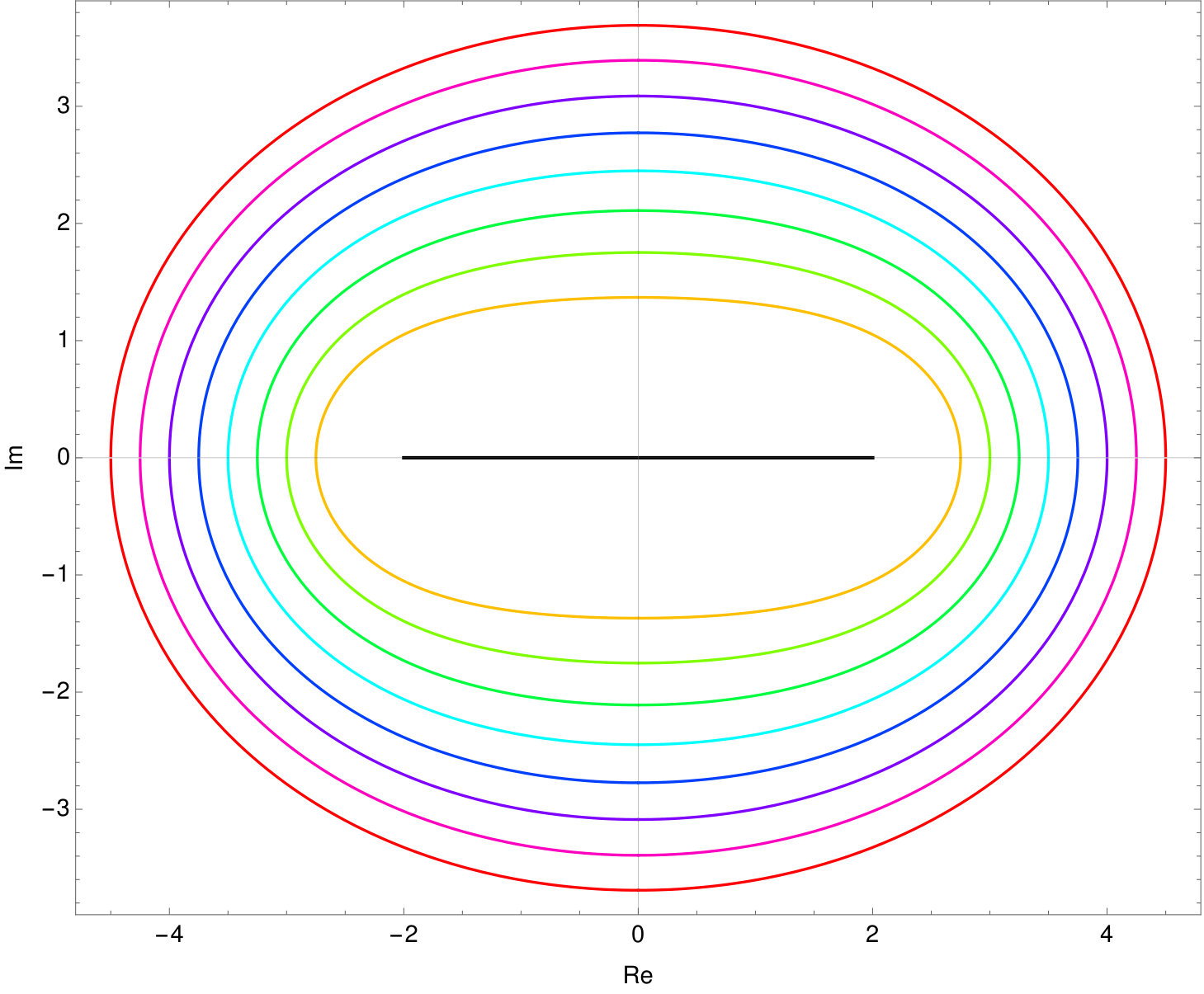 Figure 14
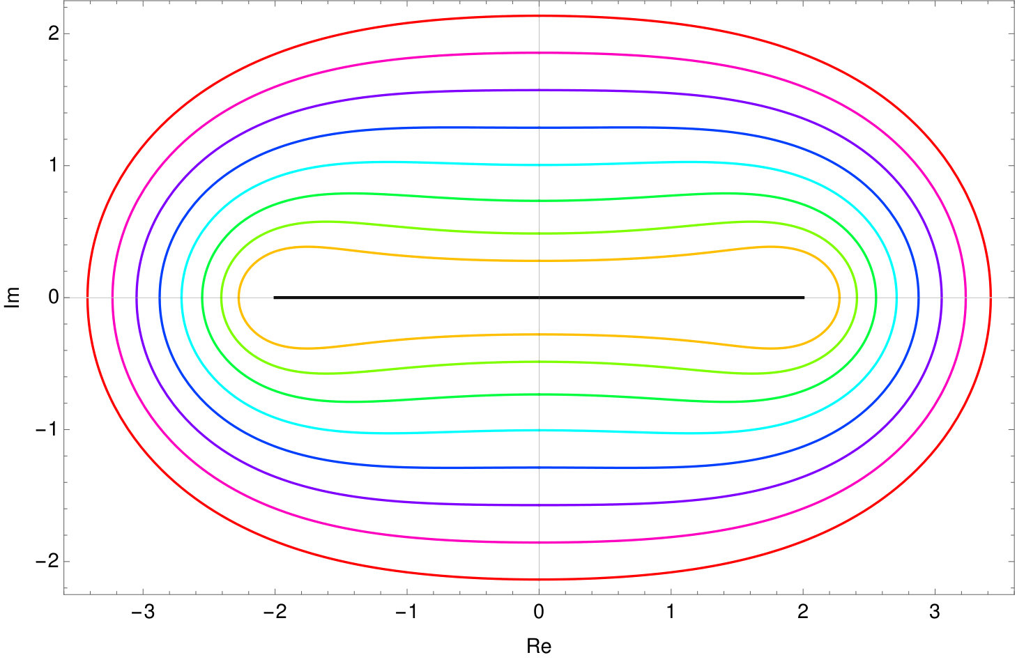 Figure 15
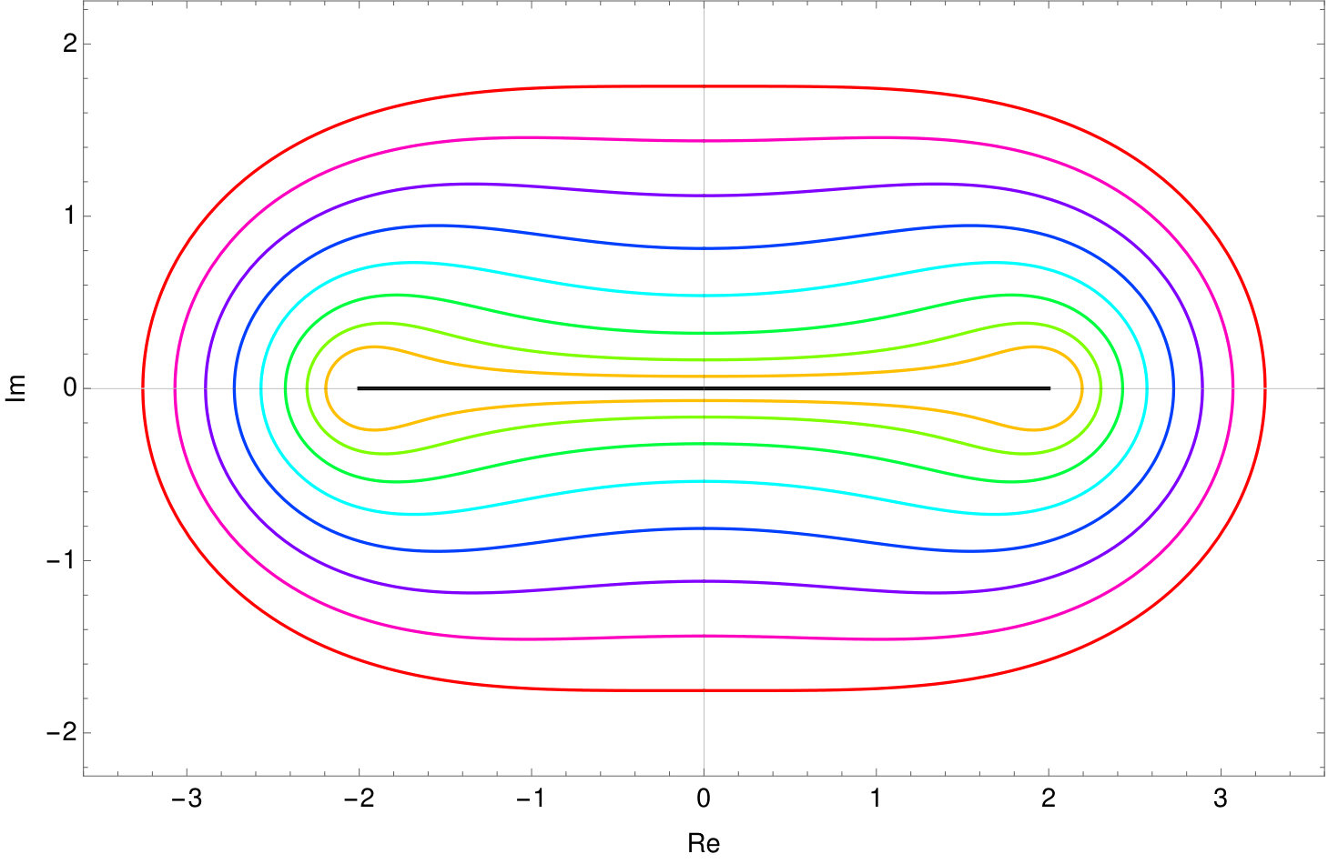 Figure 16
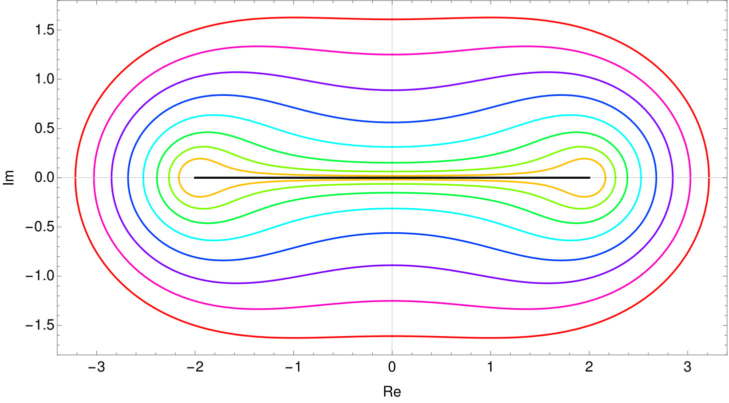 Figure 17
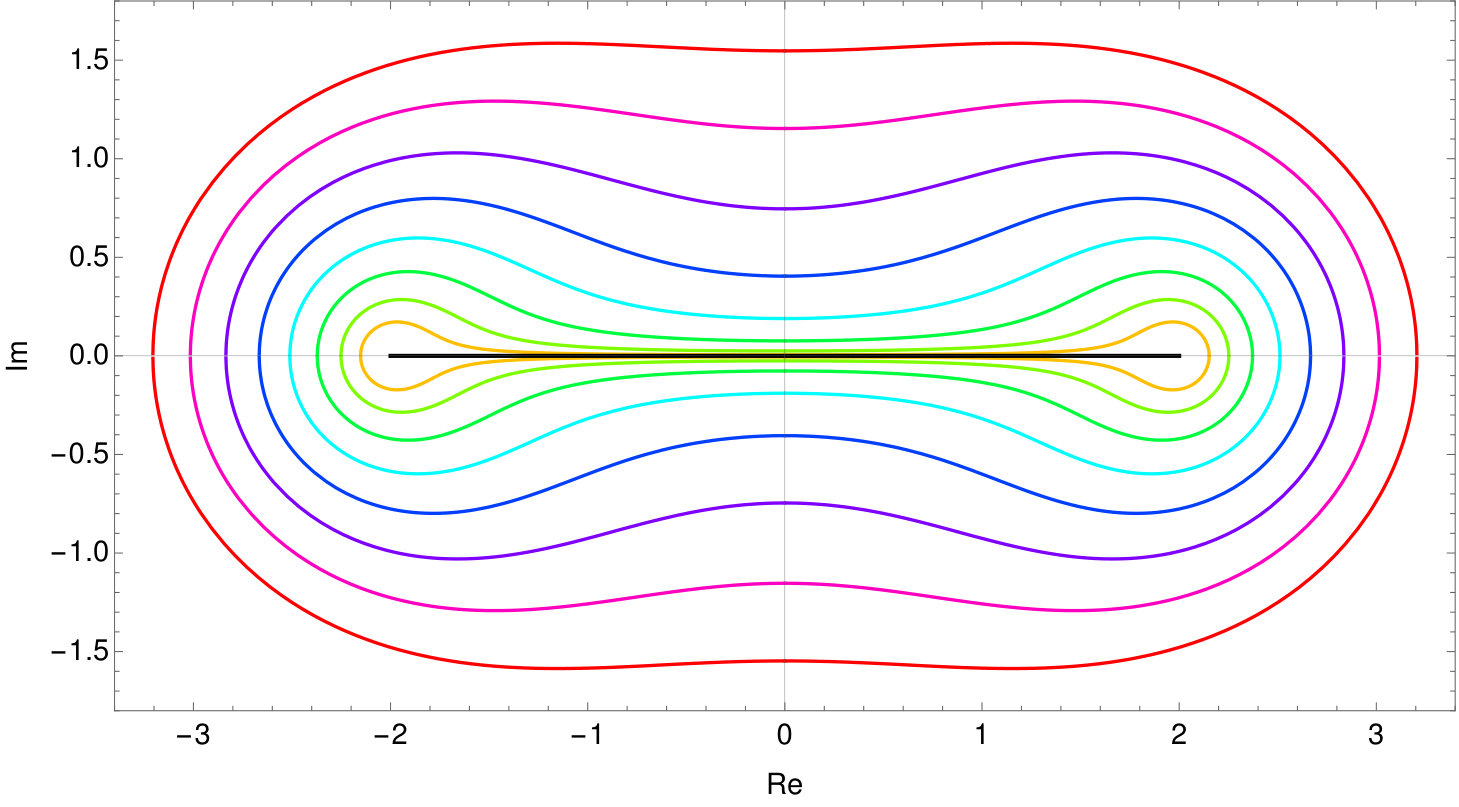 Figure 18
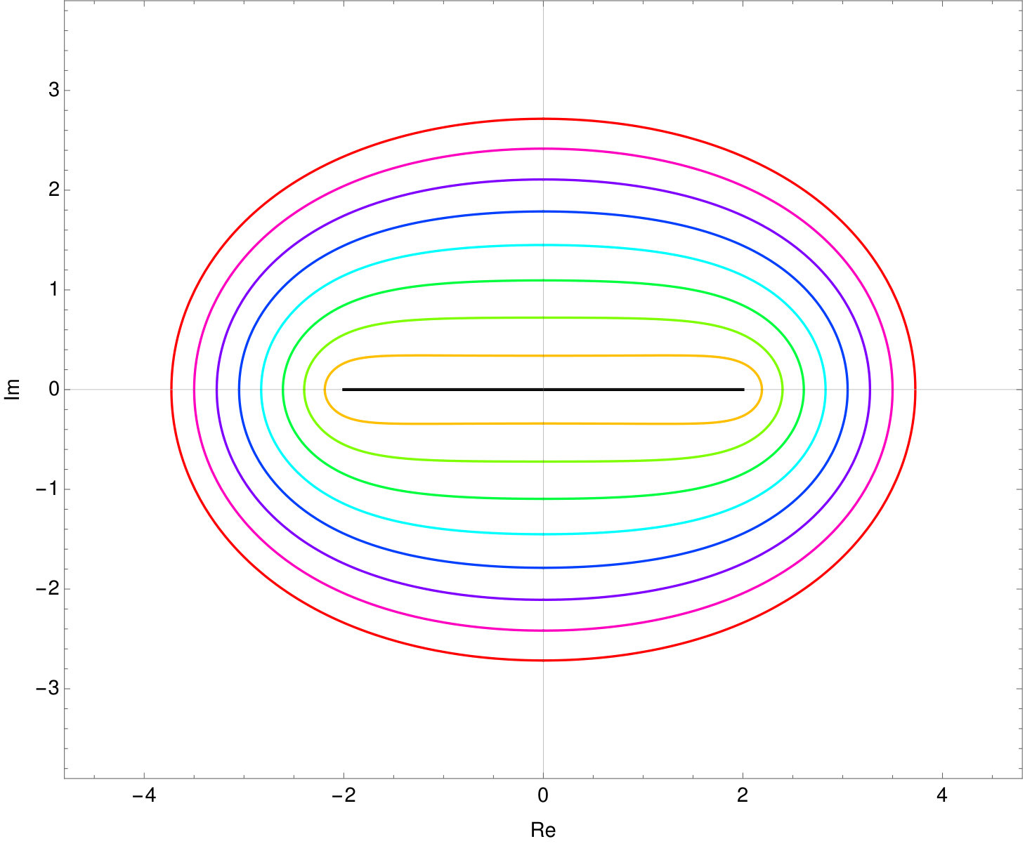 Figure 19
Peer Reviews
No public reviews on file for this paper yet. If you reviewed it on a platform where reviews are public (OpenReview, ICLR, NeurIPS, ICML), you can paste yours below so the community can read it here.
Videos
No videos yet. Explain this paper in a talk, walkthrough, or lecture? Add one.
Spectral enclosures for non-self-adjoint
discrete Schrödinger operators
Orif O. Ibrogimov
Department of Mathematics, Faculty of Nuclear Sciences and Physical Engineering, Czech Technical University in Prague, Trojanova 13, 12000 Praha 2, Czech Republic
and
František Štampach
Department of Applied Mathematics, Faculty of Information Technology, Czech Technical University in Prague, Thákurova 9, 160 00 Praha, Czech Republic
Abstract.
We study location of eigenvalues of one-dimensional discrete Schrödinger operators with complex -potentials for . In the case of -potentials, the derived bound is shown to be optimal. For , two different spectral bounds are obtained. The method relies on the Birman–Schwinger principle and various techniques for estimations of the norm of the Birman–Schwinger operator.
Key words and phrases:
Discrete Schrödinger operator, Birman-Schwinger principle point spectrum, Jacobi matrix.
2010 Mathematics Subject Classification:
34L15, 47B36, 47A75
1. Introduction and main results
Recent years have seen a significant development in the spectral theory of non-self-adjoint operators. A great deal of research aims to a localization of spectra of differential operators such as Schrödinger operators [1, 3, 9, 12, 16, 19, 20, 23, 21, 30, 31, 33, 22, 18, 25, 29], Dirac operators [6, 10, 17] and others [8, 27, 24]. For related recent results obtained in an abstract operator theoretic setting, the reader may also consult [2, 11, 13, 14].
In contrast to the differential operators, there are almost no works studying similar questions for their discrete analogues, i.e. the difference operators like discrete Schrödinger or discrete Dirac operators with complex potentials. The authors are only aware of [26] which is focused on the number rather than the location of eigenvalues for the discrete Schrödinger operator with a complex potential and a related work [28] for the cubic lattice. Some constrains on the location of the discrete spectrum of semi-infinite complex Jacobi matrices are discussed in [15].
Our main interest is to bridge this gap focusing first on the location of spectrum of the one-dimensional dicrete Schrödinger operator with a complex valued -potential, , which is the objective of this paper. The one-dimensional Dirac operator with a complex potential is discussed in a separate paper [4].
Let be the discrete Laplacian acting on the Hilbert space which is the bounded operator determined by the equation
[TABLE]
where stands for the standard basis of . Further, to a given complex sequence , we define the potential as a diagonal operator
[TABLE]
The matrix representation of the discrete Schrödinger operator is the doubly-infinite Jacobi matrix
[TABLE]
It is well known that the spectrum of the unperturbed operator is absolutely continuous and covers the interval . If the potential vanishes at infinity, i.e. as , then is compact and the essential spectrum of the perturbed operator coincides with the interval .
The goal of the present paper is to investigate the location of the spectrum of with an –potential for . Our primary result concerns the location of eigenvalues of with an –potential. Moreover, the obtained bound is shown to be optimal; see Theorem 1. If the decay of the potential is slower, namely if for , we derive bounds for the entire spectrum of ; see Theorems 2 and 3.
Theorem 1**.**
Let . Then
[TABLE]
The bound in (1.1) is sharp in the following sense: For any and any point which fulfills the equation
[TABLE]
there exists such that and is an eigenvalue of the corresponding discrete Schrödinger operator , see Section 4. This means that every boundary point of the spectral enclosure (1.1), with the exception of points located in , is an eigenvalue of for some –potential . Hence the obtained spectral bound cannot be squeezed any further.
Clearly, the geometry of the spectral enclosure (1.1) depends on the -norm of the potential. If , the spectral enclosure consists of two connected components each containing either the point or . If , the spectral enclosure is a connected set containing the entire interval . The set is always symmetric with respect to both the real and the imaginary axes, see Figure 1 in Section 5.
Our next result provides a spectral estimate in terms of the -norm of the potential. In the sequel, for , we denote by the corresponding Hölder exponent, i.e. if and if .
Theorem 2**.**
Let and let . Then
[TABLE]
Similarly to the continuous setting, see e.g. [21, 7], complex interpolation applied to an appropriate analytic family of Birman–Schwinger type operators yields the following alternative spectral enclosure for the case of –potentials.
Theorem 3**.**
Let and let . Then
[TABLE]
Remark 1**.**
For , the inequality in (1.3) has to be understood as
[TABLE]
Note also that, if one sets in (1.3), one arrives at the bound (1.1) without the exclusion of the interval , however.
Notice the comparatively simpler form of the spectral enclosure from Theorem 1 in comparison with the ones of Theorems 2 and 3. The spectral enclosures from (1.2) and (1.3) are compact sets which are symmetric with respect to both the real and the imaginary axes. However, in contrast to (1.1), they are always connected sets containing the entire interval . In general, none of the spectral enclosures from (1.2) and (1.3) is a subset of the other. Naturally, taking their intersection yields the best result. Several plots of boundary curves of these sets as well as their comparison are presented in Section 5.
The methodology used to deduce spectral enclosures of Theorems 1 and 2 is by no means new. It relies on the conventional Birman–Schwinger principle similarly as the analogous results for the (continuous) Schrödinger and Dirac operators, see e.g. [20, 19, 10, 17, 23] and also [11, 27]. The lastly mentioned papers served as a motivation for the current work. In comparison with the (continuous) Schrödinger operators, where the spectral enclosure is a disk centered at the origin, the spectral enclosures from Theorems 1, 2 and 3 have more interesting geometry. On the other hand, to estimate the norm of the Birman–Schwinger operator is technically less demanding in the discrete setting. Namely, it is done by elementary means in the case of –potentials, it makes use of either the Schur test or discrete Young’s inequality to deduce (1.2), or it employs a very particular form of Stein’s complex interpolation to obtain (1.3).
The outline of the paper is as follows. In Section 2, the Birman–Schwinger principle is briefly recalled. Section 3 contains proofs of Theorems 1, 2, and 3 with two alternative proofs for Theorem 2. In Section 4, we discuss an example of the operator with a delta potential which demonstrates the optimality of the spectral enclosure (1.1) for –potentials. Final Section 5 is devoted to numerical illustrations of the results of Theorems 1, 2, and 3.
2. The Birman–Schwinger principle
The central role in our analysis is played by the Birman–Schwinger operator
[TABLE]
where and with the complex signum function defined by
[TABLE]
For , the Birman–Schwinger operator is a bounded operator in and its matrix elements read
[TABLE]
Here the middle term corresponds to the matrix element of the resolvent of the discrete Laplace operator which is given by
[TABLE]
where and , see [36, Chp. 1]. Here, it is often convenient to relate the spectral parameter with by the Joukowsky transform which is a bijection between the punctured unit disk and the resolvent set of .
For and a bounded potential , the Birman–Schwinger principle is the equivalence
[TABLE]
can be easily justified by usual arguments. In particular, it follows that the implication
[TABLE]
holds true for . Moreover, the implication in (2.3) remains valid even if the spectra are replaced by point spectra. Indeed, if for some and , then simple manipulations with the eigenvalue equation yields for since is bounded by our assumption. Consequently, the Birman–Schwinger principle implies the inclusion
[TABLE]
3. Proofs
3.1. Proof of Theorem 1
The proof uses (2.5). Since the set on the right-hand side of (1.1) always contains points we can distinguish the following two cases.
Case . Let be such that and . It follows readily from (2.2) that
[TABLE]
For , the Birman–Schwinger operator is Hilbert–Schmidt (even trace class). Using (3.1) and the Cauchy–Schwarz inequality, we can estimate
[TABLE]
for any . Hence
[TABLE]
and, according to (2.5), if , then
[TABLE]
Case . We make use of the fact that assumption actually implies . This seems to be a commonly known result but we did not find an exact reference for this claim concerning doubly-infinite Jacobi matrices with complex entries. Nevertheless, it follows readily from the existence of a particular solution of the three-term recurrence
[TABLE]
which satisfies
[TABLE]
provided that . The solution is referred to as the Jost solution and its existence is proved, for example, in [34, Sec. 13.6] for real valued . However, the reality of the potential is of no importance for the proof and hence the statement can be extended to complex valued as well.
If and , then but . Consequently, the Jost solution exists. Moreover, the second linearly independent solution of (3.4) can be chosen as since the Wronskian
[TABLE]
where we have used (3.5) and the fact that . Consequently, any solution of the eigenvalue equation , for , is a linear combination of and where and . Such is square summable only if trivial. Thus cannot be an eigenvalue of . This completes the proof. ∎
3.2. Proof of Theorem 2
Let be such that and . It follows readily from (2.2) that
[TABLE]
There are at least two proofs of Theorem 2. The first one makes use of a slight modification of the classical Schur test adjusted to our needs. The classical Schur test can be found in [5, Exer. 9, Chp. II].
Lemma 1** (Schur test).**
Let be a bounded operator on with matrix entries with respect to the standard basis denoted by for . Suppose that there is a set such that whenever or . Then, for arbitrary weights , , one has
[TABLE]
The second proof applies discrete Young’s inequality which can be proved by a simple modification of the proof of classical Young’s inequality [32, Thm. 4.2].
Theorem 4** (discrete Young’s inequality).**
Let be such that
[TABLE]
Then, for any , , and , one has
[TABLE]
The first proof of Theorem 2.
We apply the Schur test to the Birman–Schwinger operator defined in (2.1). Since whenever or , we put and the positive weights are chosen as for . Then, taking the definition (2.1) and (3.6) into account, we obtain the estimate
[TABLE]
For the case , we infer from (3.8) that
[TABLE]
Now consider the case . For every fixed , Hölder’s inequality yields
[TABLE]
and thus
[TABLE]
In view of the estimates (3.9) and (3.11), the Birman–Schwinger principle (2.3) thus implies that cannot belong to the spectrum of unless it holds that
[TABLE]
Finally, noticing that also the interval is always included in the set on the right-hand side of (1.2), corresponding to the case when , the proof is completed. ∎
The second proof of Theorem 2.
Suppose for and and , , such that . For , we have
[TABLE]
where
[TABLE]
Notice that, by Hölder’s inequality, we have
[TABLE]
Moreover, for any , it is clearly true that
[TABLE]
Thus, we can apply Young’s inequality (3.7) in (3.13) with the indices and replaced by (or by if ) and is the Hölder dual index to ( if ). Taking also (3.14) and (3.15) into account, we obtain the estimate
[TABLE]
for all . In other words, we arrived at (3.11) again and the same reasoning as in the previous proof implies the desired inclusion (2.4). ∎
3.3. Proof of Theorem 3
The proof makes use of Stein’s complex interpolation theorem, see [35, Thm. 1]. However, only a special version of the theorem is sufficient for our needs. Its statement is as follows.
Theorem 5** (Stein’s interpolation).**
Let be a family of operators analytic in the strip and continuous and uniformly bounded in its closure . Suppose further that there exist constants and such that
[TABLE]
for all . Then, for any , one has
[TABLE]
Proof of Theorem 3.
Let be fixed. If , one readily estimates the Birman–Schwinger operator getting
[TABLE]
Then (2.4) implies (1.3) in the particular case .
Suppose . Define the operator family
[TABLE]
for with . Note that is continuous in the closed strip and analytic in its interior. Moreover, estimating similarly as above, we get
[TABLE]
Therefore, is uniformly bounded for .
Further, since by the hypothesis, we have . Consequently, we can apply (3.2) to get
[TABLE]
for any . Moreover, for all , we have also the trivial estimate
[TABLE]
Hence, we may apply Theorem 5 with which yields
[TABLE]
and (2.4) completes the proof. ∎
4. Optimality of the eigenvalue bound for -potentials
In this section, we demonstrate that the result (1.1) is sharp in the sense that to any boundary point of the spectral enclosure which is not located in , there exists an –potential so that this boundary point is an eigenvalue of . The excluded boundary points occur only if and they are .
For this purpose, we consider the operator with the potential determined by the sequence
[TABLE]
where is a coupling constant and stands for the Kronecker delta. The eigenvalue equation reads
[TABLE]
It is convenient to write for . Such exists unique inside the unit disk if , there are exactly two on the unit circle , if , and if . In any case, one readily verifies that the vector
[TABLE]
fulfills the eigenvalue equation
[TABLE]
If, in addition, , then and hence
[TABLE]
Obviously, and thus the eigenvalue is a boundary point of the spectral enclosure from (1.1). Moreover, let us remark that, in this particular example, the Birman–Schwinger operator takes the simple form
[TABLE]
for with . Thus the Birman–Schwinger principle (2.3) together with the fact that shows
[TABLE]
where if and only if , in which case .
On the contrary, it is not difficult to see that to any boundary point of the spectral enclosure (1.1) for with , there exists with and such that and Hence, if we put , the previous analysis shows that is an eigenvalue of with the potential given by the sequence (4.1).
5. Plots of the spectral enclosures from Theorems 1, 2, and 3
First Figure 1 shows the spectral enclosures from Theorem 1.
Second, we provide several plots as an illustration of the spectral enclosures from Theorem 2 in Figure 2. Denoting by , the set in (1.2) is determined by two parameters and . Without going into details, we remark that the boundary curve given by the equation
[TABLE]
for , can be parametrized in the first quadrant ( and ) as
[TABLE]
for , where and are the unique solutions of the equations
[TABLE]
for , respectively. This parametrization is used in the plots in Figure 2.
Third set of plots shows the spectral enclosures from Theorem 3, see Figure 3. Finally, we compare the spectral enclosures from Theorems 2 and 3 for six values of in Figure 5. The plots indicate that, for general , no spectral enclosure is a subset of the other one.
Acknowledgement
The first author thanks Prof. David Krejčiřík for stimulating discussions. The second author acknowledges financial support by the Ministry of Education, Youth and Sports of the Czech Republic project no. CZ.02.1.01/0.0/0.0/16_019/0000778.
The reference list from the paper itself. Each links out to its DOI / PubMed record.
- 1[1] A. A. Abramov, A. Aslanyan, and E. B. Davies, Bounds on complex eigenvalues and resonances , J. Phys. A 34 (2001), no. 1, 57–72.
- 2[2] J. Behrndt, M. Langer, V. Lotoreichik, and J. Rohleder, Spectral enclosures for non-self-adjoint extensions of symmetric operators , J. Funct. Anal. 275 (2018), no. 7, 1808–1888.
- 3[3] S. Bögli, Schrödinger operator with non-zero accumulation points of complex eigenvalues , Comm. Math. Phys. 352 (2017), no. 2, 629–639.
- 4[4] B. Cassano, O. O. Ibrogimov, D. Krejčiřík, and F. Štampach, Location of eigenvalues of non-self-adjoint discrete Dirac operators , ar Xiv:1910.10710[math.SP] (2019).
- 5[5] J. B. Conway, A course in functional analysis , second ed., Graduate Texts in Mathematics, vol. 96, Springer-Verlag, New York, 1990. MR 1070713
- 6[6] J.-C. Cuenin, Estimates on complex eigenvalues for Dirac operators on the half-line , Integr. Equ. Oper. Theory 79 (2014), no. 3, 377–388.
- 7[7] by same author, Eigenvalue bounds for Dirac and fractional Schrödinger operators with complex potentials , J. Funct. Anal. 272 (2017), no. 7, 2987–3018.
- 8[8] by same author, Sharp spectral estimates for the perturbed Landau Hamiltonian with L p superscript 𝐿 𝑝 L^{p} potentials , Integr. Equ. Oper. Theory 88 (2017), no. 1, 127–141.