Virtual Enriching Operators
Susanne C. Brenner, Li-yeng Sung

TL;DR
This paper introduces bounded linear operators that transform $H^1$ finite element spaces into $H^2$ virtual element spaces, aiding the analysis of advanced finite element methods in 2D and 3D.
Contribution
It constructs new operators bridging $H^1$ and $H^2$ spaces, enhancing the theoretical framework for nonstandard finite element analysis.
Findings
Operators are bounded and linear.
Applicable in 2D and 3D finite element contexts.
Facilitates analysis of nonstandard methods.
Abstract
We construct bounded linear operators that map conforming Lagrange finite element spaces to conforming virtual element spaces in two and three dimensions. These operators are useful for the analysis of nonstandard finite element methods.
Click any figure to enlarge with its caption.
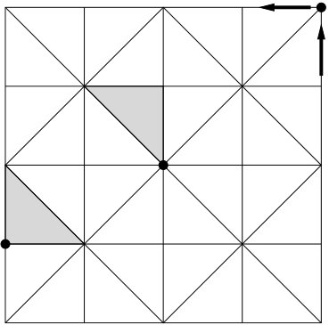 Figure 1
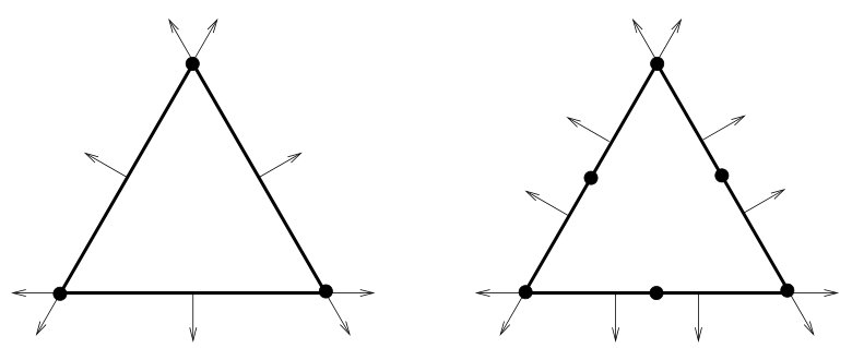 Figure 2
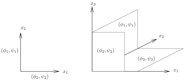 Figure 3
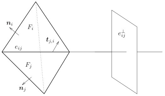 Figure 4
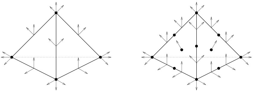 Figure 5
Peer Reviews
No public reviews on file for this paper yet. If you reviewed it on a platform where reviews are public (OpenReview, ICLR, NeurIPS, ICML), you can paste yours below so the community can read it here.
Videos
No videos yet. Explain this paper in a talk, walkthrough, or lecture? Add one.
Virtual Enriching Operators
Susanne C. Brenner
Susanne C. Brenner, Department of Mathematics and Center for Computation and Technology, Louisiana State University, Baton Rouge
and
Li-yeng Sung
Li-yeng Sung, Department of Mathematics and Center for Computation and Technology, Louisiana State University, Baton Rouge, LA 70803, USA
Abstract.
We construct bounded linear operators that map conforming Lagrange finite element spaces to conforming virtual element spaces in two and three dimensions. These operators are useful for the analysis of nonstandard finite element methods.
This work was supported in part by the National Science Foundation under Grant No. DMS-16-20273.
1. Introduction
Let () be a bounded polygonal/polyhedral domain, be a simplicial triangulation of and be the Lagrange finite element space with . The mesh dependent semi-norm is defined by
[TABLE]
where is the piecewise Hessian of with respect to , and
[TABLE]
Here (resp., ) is the set of interior edges (resp., faces) of , (resp., ) is the diameter of the edge (resp., face ), is the jump of the normal derivative across an edge (resp., face ), and (resp., ) is the infinitesimal length (resp., area).
Our goal is to construct a linear operator such that
[TABLE]
where is the Lagrange nodal interpolation operator, and the positive constants and only depend on the shape regularity of and . Moreover, the operator maps into .
Enriching operators that satisfy (1.4) and (1.5) are useful for a priori and a posteriori error analyses for fourth order elliptic problems [8, 17, 6, 7, 9], and they also play an important role in fast solvers for fourth order problems [4, 5, 10]. A recent application to Hamilton-Jacobi-Bellman equations can be found in [21].
In the two dimensional case, one can construct through the macro finite elements in [14, 13, 23, 22, 15]. This was carried out in [8] for the quadratic element and in [17] for higher order elements. However macro elements of order higher than 3 are not available in three dimensions and therefore this approach can only be carried out for quadratic and cubic Lagrange elements (cf. [21]) using the three dimensional cubic Clough-Tocher macro element from [25].
We take a different approach in this paper by connecting the -th order Lagrange finite element space to a -th order conforming virtual element space. In two dimensions such spaces are already in the literature [11, 12], and we will develop a version of three dimensional conforming virtual element spaces that are sufficient for the construction of .
Remark 1.1**.**
The assumption that the order of the Lagrange finite element space is at least 3 allows a uniform construction of . For the quadratic Lagrange finite element space we can simply take to be the restriction of the cubic enriching operator.
The rest of the paper is organized as follows. The construction of in two dimensions is carried out in Section 2, followed by the construction in three dimensions in Section 3 and some concluding remarks in Section 4. Appendix A contains some technical results concerning inverse trace theorems that are needed for the construction of conforming virtual elements.
A list of notations and conventions that will be used throughout the paper is provided here for convenience.
- •
A polygon/polyhedron is an open subset in , an edge of a polygon/polyhedron does not include the endpoints and a face of a polyhedron does not include the vertices and edges. These conventions apply in particular to triangles and tetrahedra.
- •
Let be an open line segment, a triangle or a tetrahedron, and be an integer. is the space of polynomials of total degree restricted to if and if . We say that two functions and defined on have identical moments up to order if the integral of on vanishes for all . The orthogonal projection from onto is denoted by .
- •
is the set of all the vertices of the triangles/tetrahedra in , is the set of vertices in and is the set of vertices on .
- •
is the set of all the edges of the triangles/tetrahedra in , is the set of edges in and is the set of edges that are subsets of .
- •
is the set of all the faces of the tetrahedra in , is the set of faces in and is the set of faces that are subsets of .
- •
is the set of all the triangles/tetrahedra in that share as a common vertex.
- •
is the set of all the triangles/tetrahedra in that share as a common edge.
- •
is the set of all the tetrahedra in that share as a common face.
- •
is the set of the faces of the tetrahedra in that share as a common edge.
- •
If is a function defined on a triangle/tetrahedron, then (resp., ) is the restriction of to an edge (reps., a face ).
- •
If is a function defined on a triangle/tetrahedron, then denotes the outward normal derivative of along . In the case of a triangle (resp. tetrahedron), is double-valued at the vertices (resp., edges) of .
- •
If is an edge of the triangle , then is the unit vector orthogonal to and pointing towards the outside of . If is an edge of a face of a tetrahedron , then is the unit vector tangential to , orthogonal to and pointing towards the outside of .
- •
If is a face of the tetrahedron , then is the unit vector orthogonal to and pointing towards the outside of .
2. The Two Dimensional Case
The construction of is based on the characterizations of trace spaces associated with a triangle and the construction of polynomial data on the skeleton of that satisfy these characterizations on all the triangles of .
2.1. Trace Spaces for a Triangle
Let be a triangle with vertices , and , be the edge of opposite , be the unit outer normal along , and be the counterclockwise unit tangent of . Let be a nonnegative number. A function belongs to the piecewise Sobolev space if and only if , the restriction of to , belongs to for . It follows from the Sobolev Embedding Theorem [1, Theorem 4.12] that we can define a linear operator by
[TABLE]
where the restrictions of and are in the sense of trace and defined piecewise with respect to the edges. For the subspace of , we have . Our first task is to identify the image of .
Definition 2.1**.**
A pair belongs to the space if and only if the following conditions are satisfied:
[TABLE]
Note that the compatibility conditions (2.3)–(2.4) are equivalent to
[TABLE]
for and .
It follows from the Sobolev Embedding Theorem that for , where , and we can recover on from by
[TABLE]
We want to show that in fact . For this purpose it is useful to construct a linear isomorphism such that
[TABLE]
where is an orientation preserving affine transformation that maps the triangle onto . We assume that maps the vertex of to the vertex of and hence it also maps the edge of to the edge of .
First we note that, by the chain rule,
[TABLE]
where (a constant matrix with a positive determinant) is the Jacobian of .
Let . Motivated by (2.6)–(2.8), we define , where
[TABLE]
and
[TABLE]
where is the outward pointing unit normal along the edge and the vector field on is given by
[TABLE]
It is straightforward to check that , is a bijection, and that (2.7) follows from (2.6) and (2.8)–(2.11).
We are now ready to characterize .
Lemma 2.2**.**
The image of under is the space .
Proof.
We already know that . In the other direction, we want to construct that satisfies (2.1) for a given .
If and vanish near the vertices, we can use the operator in Lemma A.1 and cut-off functions to obtain . Therefore, by using a partition of unity, we can reduce the construction to a neighborhood of a vertex and, by an affine transformation (cf. (2.7)), we can further assume that the angle at the vertex is a right angle. The existence of near such a vertex then follows from Lemma A.3. ∎
2.2. Affine Invariant Virtual Element Spaces
The construction of the virtual element spaces involves polynomial subspaces of .
Definition 2.3**.**
Let be a triangle. We will denote the intersection of and by .
Remark 2.4**.**
It follows from the compatibility conditions (2.2)–(2.4) that is determined by (i) the values of at the vertices, (ii) the tangential derivatives of at the vertices, (iii) moments of on up to order that together with (i) and (ii) determine , and (iv) moments of up to order that together with (ii) (through (2.4)) determine . These degrees of freedom (dofs) are depicted in Figure 2.1 for and , where (i) the values of at the vertices and the moments of on the edges are represented by solid dots, and (ii) the tangential derivatives of at the vertices and the moments of on the edges are represented by arrows. Altogether we have .
Remark 2.5**.**
Since polynomial spaces are preserved by an affine transformation, the map defined by (2.9)–(2.10) maps one-to-one and onto .
2.2.1. Virtual Element Spaces on the Reference Triangle
We begin with a simple well-posedness result for the biharmonic problem.
Lemma 2.6**.**
Given any and , there exists a unique such that
[TABLE]
Proof.
Let satisfy (2.1) and be defined by
[TABLE]
Then is the unique solution of (2.6). ∎
Let be the reference triangle with vertices , and . In view of Lemma 2.6 and the fact that is a subspace of , we can now define the reference virtual element spaces , which are identical to the virtual element spaces in [11] for the special case of the reference triangle.
Definition 2.7**.**
A function belongs to the virtual element space if and only if and the distributional derivative belongs to , i.e., there exists such that
[TABLE]
Remark 2.8**.**
According to Remark 2.4 and Lemma 2.6, we have
[TABLE]
The following result is well-known (cf. [11]). We provide a proof here for self-containedness.
Lemma 2.9**.**
A function in is uniquely determined by and .
Proof.
In view of Remark 2.8, it suffices to show that is the only function in with the properties that and . Indeed, using integration by parts and the fact that the distributional derivative , we have
[TABLE]
Therefore is a harmonic function that vanishes on and hence . ∎
Remark 2.10**.**
The definition of the virtual element space relies on the fact that is a subspace of . One can show by using macro elements of order that a pair satisfying the compatibility conditions (2.2)–(2.4) automatically belongs to . Hence Lemma 2.2 is not necessary for the definition of the virtual element space in two dimensions. However, the definition of the virtual element spaces in three dimensions requires the characterization of the trace of for the reference tetrahedron , since macro elements of arbitrary order are not available. The approach here provides a preview of the three dimensional case.
2.2.2. Virtual Element Spaces for a General Triangle
We now define for an arbitrary triangle in terms of .
Definition 2.11**.**
Let be an arbitrary triangle and be an orientation preserving affine transformation that maps onto . Then if and only if .
Remark 2.12**.**
The definition of is independent of the choice of . The polynomial space is a subspace of since is obviously a subspace of . The dimension of is also given by the formula in (2.14).
We have an analog of Lemma 2.9.
Lemma 2.13**.**
A function in is uniquely determined by and .
Proof.
This is a direct consequence of (2.7), Remark 2.5, Lemma 2.9 and the relation . ∎
Remark 2.14**.**
Our definition of , which is invariant under affine transformations, differs from the one in [11] for a general triangle. The affine invariance simplifies the proofs of (1.4) and (1.5) in Section 2.4. We note that it is also possible to use the virtual finite element spaces from [11] in the construction of . But then the proofs of (1.4) and (1.5) will become more involved.
Remark 2.15**.**
The definition of virtual element spaces on polygons and their applications to the plate bending problem can be found in [11, 12].
2.3. Construction on the Skeleton
Given , our goal is to define representing (the desired) E_{h}v\big{|}_{\partial T} and representing (the desired) (\partial E_{h}v/\partial n)\big{|}_{\partial T} for all , such that
[TABLE]
and the following conditions are satisfied:
[TABLE]
Note that (2.16) and (2.17) imply any piecewise function satisfying (\xi_{T},\partial\xi_{T}/\partial n)\big{|}_{\partial T}=(f_{v,{\scriptscriptstyle T}},g_{v,{\scriptscriptstyle T}}) for all will belong to , and (2.18) implies that if .
2.3.1. Construction at the Vertices
In view of the compatibility conditions (2.3) and (2.4), we need to define vectors associated with the vertices of . There are three cases: (i) is an interior vertex, (ii) is boundary vertex that is not a corner of and (iii) is a corner of .
Case (i) For an interior vertex , we define to be , where is any triangle in .
Case (ii) For a boundary vertex that is not a corner of , we define to be , where is one of the triangles in that has an edge on . This choice ensures that if , where is any vector tangential to at .
Case (iii) At a corner of , we define by
[TABLE]
where are the two edges emanating from and is the derivative in the direction of the unit tangent of . Note that at a corner of if .
The choices of the triangles and tangent vectors in Case(i)–Case(iii) are illustrated in Figure 2.2.
Remark 2.16**.**
If the condition
[TABLE]
is satisfied at a vertex , then obviously for all .
2.3.2. Construction on the Edges
On any edge , we define a polynomial as follows: First we choose and then we specify that
[TABLE]
2.3.3. Construction on the Triangles
We are now ready to define for any as follows. Given any edge of , the function on is the unique polynomial in with the following properties:
[TABLE]
Remark 2.17**.**
If the condition (2.20) is satisfied at both endpoints of , then at the two endpoints of by Remark 2.16 and then conditions (2.23) and (2.24) imply on .
Given any edge of , we define
[TABLE]
Remark 2.18**.**
If the condition (2.20) is satisfied at both endpoints of and is across , then Remark 2.16 and (2.21)–(2.22) imply that on .
By construction, the condition (2.15) is satisfied because the compatibility conditions (2.2)–(2.4) follow from (2.21) and (2.23)–(2.24). The condition (2.16) follows from (2.23)–(2.24) and the condition (2.17) follows from (2.25). The choices we make in the definition of for (cf. Case (ii) and Case (iii) in Section 2.3.1 and (2.23)–(2.24)) also implies (2.18).
2.4. The Operator
Let and be arbitrary, and be the function pair constructed in Section 2.3. We define by the following conditions (cf. Lemma 2.13):
[TABLE]
It follows from (2.16)–(2.17) that the piecewise function belongs to , and (2.18) implies if . It only remains to establish the estimates (1.4) and (1.5).
Note that Remark 2.17 and Remark 2.18 imply
[TABLE]
and hence if is on , which is the rationale behind (1.4) and (1.5).
Theorem 2.19**.**
The estimate (1.4) holds with a positive constant that only depends on and the shape regularity of .
Proof.
All the constants (explicit or hidden) that appear below will only depend on the minimum angle of .
Let be arbitrary. In view of Remark 2.4, Lemma 2.13 and the equivalence of norms on finite dimensional vector spaces, we have, by scaling,
[TABLE]
where is the diameter of and (resp., ) is the set of the three vertices (resp., edges) of . Moreover the affine invariance of (cf. Definition 2.11) together with (2.10) and (2.11) implies that the hidden constants in (2.28) only depend on the shape regularity of .
It follows from (2.23), (2.26) and (2.28) that
[TABLE]
and we also have, by the construction of in Section 2.3.1, (2.22), (2.24), and (2.25),
[TABLE]
where is the set of all the edges in that share as a common vertex, and hence
[TABLE]
We then deduce from (2.30) and scaling that
[TABLE]
Note that, because of the affine invariance of , the scaling constants behind (2.31) only depend on the shape regularity of .
The estimate (1.4) follows immediately from (1.1) and (2.31). ∎
Theorem 2.20**.**
The estimate (1.5) holds with a positive constant that only depends on and the shape regularity of .
Proof.
Let be arbitrary and (the star of ) be the interior of the union of the closures of all the triangles in that share a common vertex with . If belongs to , then in and hence on by (2.30). The estimate (1.5) can then be established through the Bramble-Hilbert lemma [3, 16]. ∎
3. The Three Dimension Case
The construction of in three dimensions follows the same strategy as in Section 2, and our treatment will be brief regarding the results and arguments that are (almost) identical with the two dimensional case.
3.1. Trace Spaces for a Tetrahedron
Let be a tetrahedron with vertices , and be the face of opposite . Let be a nonnegative number. A function belongs to the piecewise Sobolev space if and only if , the restriction of to , belongs to for .
For a function defined on a face of the tetrahedron , the planar gradient is defined by
[TABLE]
where is any extension of to a neighborhood of in .
The operator is again defined by (2.1) in a piecewise sense. We want to characterize the image of in under the operator , for which we will need more notations and definitions.
The common edge of and is denoted by and denotes the two dimensional subspace of perpendicular to . The outward unit normal on is denoted by , and we denote by the unit vector tangential to , perpendicular to and pointing outside (cf. Figure 3.1).
Definition 3.1**.**
The space consists of all vector functions defined on with image in such that for all .
Definition 3.2**.**
A pair belongs to the space if and only if the following conditions are satisfied
[TABLE]
Note that we can replace the compatibility conditions (3.2)–(3.3) by the condition
[TABLE]
It follows from the Sobolev Embedding Theorem that for , where is the orthogonal projection of along onto the subspace , and we can recover on from through the relation
[TABLE]
We want to show that .
Again we construct a linear bijection so that (2.7) is valid, where is an orientation preserving affine transformation that maps the tetrahedron onto . Let . Motivated by (2.7), (2.8) and (3.4), we define , where is given by (2.9), is given by (2.10) (where is the outward pointing unit normal along the face ) and the vector field on is given by
[TABLE]
It is straightforward to check that , is a bijection, and that (2.7) follows from (2.8)–(2.10), (3.5) and (3.6).
We can now establish the following analog of Lemma 2.2.
Lemma 3.3**.**
The image of under is the space .
Proof.
Given that satisfies (3.1)–(3.3), we can reduce the construction of to the following three cases by a partition of unity. (i) and vanish near the vertices of and the edges of , in which case we can use the operator in Lemma A.2 to obtain . (ii) and are supported in a neighborhood of an edge and vanish near the vertices of , in which case we can assume through an affine transformation (cf. (2.7)) that the dihedral angle at the edge is a right angle and obtain through Lemma A.5. (iii) and are supported near a vertex of , in which case we can assume through an affine transformation that the angle at the vertex is a solid right angle and obtain through Lemma A.4. ∎
3.2. Affine Invariant Virtual Element Spaces
We will use the same notation to denote for a tetrahedron . But the definition of is different.
Definition 3.4**.**
Let be a tetrahedron. A pair belongs to if and only if for .
Remark 3.5**.**
It follows from Lemma 2.9 and the constraints (3.1)–(3.3) that we need the following dofs for : (i) The value of at each vertex together with the values of the three directional derivatives along the three edges emanating from , which requires dofs. (ii) The moments of up to order on each edge, which together with (i) ensure the constraint (3.1). This requires dofs. (iii) The moments of order up to on each edge in order to define, together with (i), a polynomial (vector) function of order on with images in , which requires dofs. We can then use this polynomial (vector) function to define on any edge of through (3.2) and on through (3.3). (iv) On each face we need to specify the moments of and up to order in order to complete the definition of and , which requires dofs. Altogether we have
[TABLE]
The (visible) dofs of for and are depicted in Figure 3.2, where (i) the values of at the vertices and the moments of on the edges and faces are represented by solid dots, and (ii) the directional derivatives of at the vertices and the moments of on the edges and faces are represented by arrows.
The well-posedness result in Lemma 2.6 remains valid for a tetrahedron and the definition of the virtual element space on the reference tetrahedron with vertices , , and is identical to the one in Definition 2.7 for the reference triangle. The virtual element space for an arbitrary tetrahedron is then defined as in Definition 2.11 through an orientation preserving affine transformation that maps onto , and Lemma 2.9 also holds for a tetrahedron.
The dimension of is now given by
[TABLE]
Remark 3.6**.**
The definition of for a tetrahedron relies crucially on the fact that boundary data satisfying the compatibility condition (3.1)–(3.3) will belong to . Unlike the two dimensional case (cf. Remark 2.10), this cannot be taken for granted since macro elements of arbitrary order that share the same boundary data are yet to be developed.
Remark 3.7**.**
Three dimensional virtual elements on arbitrary polyhedron have recently been proposed in [2].
3.3. Construction on the Skeleton
Given any , we want to define representing (the desired) E_{h}v\big{|}_{\partial T} and representing (the desired) (\partial E_{h}v/\partial n)\big{|}_{\partial T} for all , such that
[TABLE]
and the following conditions are satisfied:
[TABLE]
Note that (3.10) and (3.11) imply any piecewise function satisfying (\xi_{T},\partial\xi_{T}/\partial n)\big{|}_{\partial T}=(f_{v,{\scriptscriptstyle T}},g_{v,{\scriptscriptstyle T}}) for all will belong to , and (3.12) implies that if .
3.3.1. Construction at the Vertices
As in Section 2.3, we first define the vectors associated with the vertices of . There are three cases: (i) is an interior vertex, (ii) is a boundary vertex that belongs to a face of , (iii) is a boundary vertex that does not belong to any face of .
Case (i) For an interior vertex , we choose a tetrahedron in and define to be .
Case (ii) For a boundary vertex that belongs to a face of , we define to be , where is a tetrahedron in that has a face on . This choice ensures that if , where is any vector tangential to at .
Case (iii) In this case is either a corner of or belongs to an edge of . We define implicitly by
[TABLE]
where , and are the tangential derivatives along three edges emanating from that are not coplanar. This choice of implies if .
Remark 3.8**.**
Note that Remark 2.16 is also valid here, i.e., for all if is at the vertex .
3.3.2. Construction on the Edges
In view of (3.2) and (3.3), we also need to define polynomial vector functions on the edges . There are three cases: (i) is an interior edge of , (ii) is a subset of a face of and (iii) is a subset of an edge of .
Case (i) Let belong to . We choose , and then define by the following conditions:
[TABLE]
Case (ii) Let be an edge of that is a subset of a face of . We define again by (3.14)–(3.15), but with the stipulation that one of the faces of is a subset of . This additional condition (together with the choices made in Cases (ii) and (iii) in Section 3.3.1) implies that on if , where is any vector tangential to .
Case (iii) Let be an edge of that is a subset of an edge of . Then there are two distinct faces and we define by (3.14) together with the condition that
[TABLE]
Our choices of and (together with the choices made in Cases (ii) and (iii) in Section 3.3.1) ensures that on if .
Remark 3.9**.**
In the case where is across an edge and at the endpoints of , it follows from Remark 3.8 and (3.14)–(3.16) that the vector field is the projection of on for all .
3.3.3. Construction on the Faces
We define on a face as follows. We choose and stipulate that
[TABLE]
Remark 3.10**.**
If is across and at the endpoints of , then we have on for all and by Remark 3.9 and (3.17).
3.3.4. Construction on the Tetrahedra
We are now ready to define for any as follows. On any edge of a face of , is the unique polynomial in with the following properties:
[TABLE]
Remark 3.11**.**
Remark 2.17 is also valid here, i.e., on if is at the endpoints of .
Let be a face of and be an edge of , we define by
[TABLE]
On each face of , the pair belongs to by (3.14) and (3.19)–(3.21). Hence we can define to be the virtual element function (cf. Lemma 2.13) that satisfies the following conditions:
[TABLE]
Remark 3.12**.**
If is on , then on by Remark 3.9 and (3.21). It then follows from Remark 2.12, Remark 3.11 and (3.22) that on .
Given any face of , we define
[TABLE]
Remark 3.13**.**
If is on , then (3.18), Remark 3.10 and (3.23) imply on .
At the end of this process, we have constructed for every polyhedron . The pair belongs to because (i) the condition (3.1) is implied by (3.19)–(3.20), (ii) the condition (3.2) is implied by (3.21)–(3.22), and (iii) the condition (3.3) is implied by (3.17).
It follows from (3.19)–(3.22) that (3.10) is satisfied, and the condition (3.11) follows from (3.23). The choices we make in Section 3.3.1 and Section 3.3.2 ensure that defined by (3.19)–(3.20) and defined by (3.21) both vanish on if the face of is a subset of and . The condition (3.12) then follows from (3.22).
In view of Remark 3.12 and Remark 3.13 the relation (2.27) remains valid, i.e., if is on , which is the basis for the estimates (1.4) and (1.5).
3.4. The Operator
We proceed as in Section 2.4. Let and be arbitrary, and be the function pair constructed in Section 3.3. We define again by the conditions in (2.26), i.e.,
[TABLE]
It follows from (3.10)–(3.11) that , and (3.12) implies that if .
The estimates (1.4) and (1.5) are established by similar arguments as in Section 2.4, where the analog of (2.28) for a tetrahedron (cf. Lemma 2.13 and Remark 3.5) is given by
[TABLE]
for all , where (resp., and ) is the set of the four faces (resp., six edges and four vertices) of and is the orthogonal projection of onto the subspace of perpendicular to . The hidden constants in (3.4) only depend on the shape regularity of because of the affine invariance of the virtual element spaces.
It follows from (3.19), (3.22), (3.24) and (3.4) that we have the following analog of (2.29):
[TABLE]
We can then establish the three-dimensional analogs of Theorem 2.19 and Theorem 2.20 as in Section 2.4.
4. Concluding Remarks
Following the approach of this paper (and with more patience and persistence), one can construct enriching operators that maps the totally discontinuous finite element space into , where (1.4) and (1.5) are valid for given by
[TABLE]
One can also construct such that (1.4) and (1.5) are valid, provided the sum in (1.2) (resp., (1.3)) is taken over (resp., ). This can also be carried out for the totally discontinuous finite element space.
Lemma 3.3 is also of independent interest, since inverse trace theorems for polyhedral domains in do not appear to be readily available in the literature.
Appendix A Inverse Trace Theorems for and
We consider inverse trace theorems for and with data on the boundaries of these domains (cf. Figure A.1). We will rely on the results in Lemma A.1 and Lemma A.2 that follow from the construction of inverse trace operators through the Fourier transform [20, 24] and the Paley-Wiener theorem [19].
Lemma A.1**.**
There exists a bounded linear operator such that , , and vanishes on the half plane if and vanish on the half line .
Lemma A.2**.**
There exists a bounded linear operator with the following properties: , , and vanishes on the half space resp., if and vanish on the half plane resp., .
We begin with a two-dimensional inverse trace theorem. We note that similar results for can be found in [18, Section 1.5.2]. Our approach is simpler (since we are considering ) and therefore its extension to three dimensions is easier.
Lemma A.3**.**
Let and belong to such that
[TABLE]
Then there exists such that
[TABLE]
Proof.
First we extend and to , so that the extensions (still denoted by and ) satisfy and . This can be achieved by reflection (cf. [20, Theorem 2.3.9] and [1, Theorem 5.19]). Let be the lifting operator in Lemma A.1 and so that
[TABLE]
Then we define , for .
Note that , and
[TABLE]
[TABLE]
by (A.2) and (A.5). Moreover we have , and
[TABLE]
by (A.3) and (A.5). Hence their trivial extensions (still denoted by and ) satisfy and .
Let such that and . Then on the half plane by Lemma A.3, which implies
[TABLE]
We can now take to be the restriction of to . ∎
Next we consider the three dimensional analog of Lemma A.3.
Lemma A.4**.**
Let , and belong to such that the following conditions are satisfied
[TABLE]
Then there exists such that
[TABLE]
Proof.
First we extend and to by reflection (twice) so that the extensions (still denoted by and ) satisfy and . Let be the lifting operator in Lemma A.2 and so that
[TABLE]
Then we define, for ,
[TABLE]
Note that belongs to and
[TABLE]
by (A.6), (A.16) and (A.18), and
[TABLE]
by (A.9), (A.17) and (A.18). Furthermore belongs to and
[TABLE]
Hence we can extend and to by reflection across (still denoted by and ) so that , , for and for . Therefore the trivial extensions of and to (still denoted by and ) belong to and respectively.
Let . Then we have, by Lemma A.2,
[TABLE]
and
[TABLE]
which implies
[TABLE]
We now define, for ,
[TABLE]
Then (resp., ) belongs to (resp., ).
Moreover, it follows from (A.8), (A.16), (A.22) and (A.23) that
[TABLE]
and (A.10), (A.17), (A.22) and (A.23) imply
[TABLE]
From (A.14), (A.16), (A.22) and (A.24) we also have
[TABLE]
Next we check the behavior of and at . We have
[TABLE]
by (A.7), (A.18), (A.20) and (A.23);
[TABLE]
by (A.11), (A.18), (A.21) and (A.23);
[TABLE]
by (A.13), (A.18), (A.20) and (A.24).
The calculations above show that on the boundary of . Hence their trivial extensions to (still denoted by and ) belongs to and .
Let . Then we have, by Lemma A.2, ,
[TABLE]
and
[TABLE]
which implies
[TABLE]
We can now take to be the restriction of to , and (A.15) follows from (A.16)–(A.27), ∎
Finally we have a three-dimensional result that is two-dimensional in nature and which can be derived by using the arguments in the proof of either Lemma A.3 or Lemma A.4.
Lemma A.5**.**
Let and belong to such that
[TABLE]
Then there exists such that
[TABLE]
The reference list from the paper itself. Each links out to its DOI / PubMed record.
- 1[1] R.A. Adams and J.J.F. Fournier. Sobolev Spaces ( ( ( Second Edition ) ) ) . Academic Press, Amsterdam, 2003.
- 2[2] L. Beirão da Veiga, F. Dassi, and A. Russo. A C 1 superscript 𝐶 1 C^{1} virtual element method on polyhedral meshes. ar Xiv:1808.01105 v 2 [math.NA], 2019.
- 3[3] J.H. Bramble and S.R. Hilbert. Estimation of linear functionals on Sobolev spaces with applications to Fourier transforms and spline interpolation. SIAM J. Numer. Anal. , 7:113–124, 1970.
- 4[4] S.C. Brenner. Two-level additive Schwarz preconditioners for nonconforming finite element methods. Math. Comp. , 65:897–921, 1996.
- 5[5] S.C. Brenner. Convergence of nonconforming multigrid methods without full elliptic regularity. Math. Comp. , 68:25–53, 1999.
- 6[6] S.C. Brenner. C 0 superscript 𝐶 0 C^{0} Interior Penalty Methods. In J. Blowey and M. Jensen, editors, Frontiers in Numerical Analysis-Durham 2010 , volume 85 of Lecture Notes in Computational Science and Engineering , pages 79–147. Springer-Verlag, Berlin-Heidelberg, 2012.
- 7[7] S.C. Brenner, J. Gedicke, L.-Y. Sung, and Y. Zhang. An a posteriori analysis of C 0 superscript 𝐶 0 C^{0} interior penalty methods for the obstacle problem of clamped Kirchhoff plates. SIAM J. Numer. Anal. , 55:87–108, 2017.
- 8[8] S.C. Brenner, T. Gudi, and L.-Y. Sung. An a posteriori error estimator for a quadratic C 0 superscript 𝐶 0 {C^{0}} interior penalty method for the biharmonic problem. IMA J. Numer. Anal. , 30:777–798, 2010.