Eigenfunction concentration via geodesic beams
Yaiza Canzani, Jeffrey Galkowski

TL;DR
This paper introduces a new technique for analyzing the concentration of Laplace eigenfunctions by decomposing them into geodesic beams, leading to improved bounds on their norms and pointwise behavior.
Contribution
The paper develops a novel method using geodesic beam decomposition to study eigenfunction concentration, providing quantitative improvements over existing bounds.
Findings
Improved bounds on $L^ Infty$ norms of eigenfunctions.
Enhanced estimates for eigenfunction averages over submanifolds.
Quantitative bounds depending on the dynamical property T.
Abstract
In this article we develop new techniques for studying concentration of Laplace eigenfunctions as their frequency, , grows. The method consists of controlling by decomposing into a superposition of geodesic beams that run through the point . Each beam is localized in phase-space on a tube centered around a geodesic whose radius shrinks slightly slower than . We control by the -mass of on each geodesic tube and derive a purely dynamical statement through which can be studied. In particular, we obtain estimates on by decomposing the set of geodesic tubes into those that are non self-looping for time and those that are. This approach allows for quantitative improvements, in terms of , on the available bounds for …
Click any figure to enlarge with its caption.
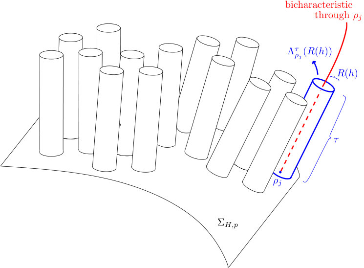 Figure 1
Peer Reviews
No public reviews on file for this paper yet. If you reviewed it on a platform where reviews are public (OpenReview, ICLR, NeurIPS, ICML), you can paste yours below so the community can read it here.
Videos
No videos yet. Explain this paper in a talk, walkthrough, or lecture? Add one.
Eigenfunction concentration via geodesic beams
Yaiza Canzani
Department of Mathematics, University of North Carolina at Chapel Hill, Chapel Hill, NC, USA
and
Jeffrey Galkowski
Department of Mathematics, University College London, London, UK
Abstract.
In this article we develop new techniques for studying concentration of Laplace eigenfunctions as their frequency, , grows. The method consists of controlling by decomposing into a superposition of geodesic beams that run through the point . Each beam is localized in phase-space on a tube centered around a geodesic whose radius shrinks slightly slower than . We control by the -mass of on each geodesic tube and derive a purely dynamical statement through which can be studied. In particular, we obtain estimates on by decomposing the set of geodesic tubes into those that are non self-looping for time and those that are. This approach allows for quantitative improvements, in terms of , on the available bounds for norms, norms, pointwise Weyl laws, and averages over submanifolds.
1. Introduction
On a smooth, compact, Riemannian manifold with no boundary, we consider sequences of Laplace eigenfunctions solving
[TABLE]
From a quantum mechanics point of view, represents the probability density for finding a quantum particle of energy at the point . As a result, understanding how concentrates across is an important problem in the mathematical physics community.
In this article, we construct tools to examine the behavior of by decomposing it into geodesic beams. To study how concentrates near , we rewrite as a sum of functions, each of which is microlocalized to a shrinking neighborhood of a geodesic that runs through . The analysis of this decomposition, including a precise description of the behavior of each geodesic beam, yields a bound on in terms of the local structure of the -mass of along each of the geodesic tubes starting at . In addition, through an application of Egorov’s theorem, we obtain estimates on the growth of that rely only on the dynamical behavior of geodesics emanating from , and not on any other geometric structure of . Throughout the article, we refer to the tools developed here as geodesic beam techniques.
The term geodesic beam is inspired by Gaussian beams. Recall that, on the round sphere, these are eigenfunctions that concentrate in a neighborhood of a closed geodesic that have a Gaussian profile transverse to the geodesic. Gaussian beams have been extensively studied in the math and physics literature (see e.g. [BL67, Arn73, KS71, BB91, DGR06, Zel15, Wei75, Ral77, Ral82]). Notably, Ralston [Ral76] constructed quasimodes associated to stable periodic orbits modelled on Gaussian beams. These references concern modes associated to a single closed geodesic. In contrast, the methods developed here decompose functions into linear combinations of what we call geodesic beams. Each building block is similar to a Gaussian beam in that it is associated to a geodesic and concentrates in a small neighborhood thereof. However, three facts crucial to our construction are: that geodesic beams are only locally defined, that the geodesic need not close, and that they do not need to have a Gaussian profile transverse to the geodesic.
In this article we build the geodesic beam tools and illustrate their application by obtaining quantitative improvements to norms for eigenfunctions on certain integrable geometries (see §5).
In addition, the techniques developed in this paper have remarkable implications in the study of norms and averages of eigenfunctions, norms, and pointwise Weyl Laws. (See §1.2, §1.3, §1.4 respectively.) However, all of these applications require some additional non-trivial input e.g. controlling looping behavior of geodesics in [CG19a], understanding the local geometry of overlapping tubes in [CG20a], and reduction of Weyl remainders to quasimode estimates in [CG20b]. We stress that the crucial technique in each application is that of geodesic beams, which are developed in this article. We briefly describe the applications to norms, averages, norms, and Weyl Laws now:
** norms:** Beginning in the 1950’s, the works of Levitan, Avakumović, and Hörmander [Lev52, Ava56, Hör68] prove the estimate as ; known to be saturated on the round sphere. This bound was improved to by Sogge, Toth, Zelditch and the second author [SZ02, STZ11, SZ16a, SZ16b, GT17, Gal19] under various dynamical assumptions at . Notably, [SZ02] was the first to study bounds under purely local dynamical assumptions. When has no conjugate points, a quantitative improvement of the form has been known since the classical work of Bérard [Bér77, Bon17, Ran78]. However, until the present time, no quantitative improvements were available without global geometric assumptions on . In §1.2 we present applications of our geodesic beam techniques giving such improvements.
Averages: Another measure of eigenfunction concentration is the average over a submanifold of codimesion . In this case, the general bound was proved by Zelditch [Zel92] and is saturated on the round sphere. This generalized the work of Good and Hejhal [Goo83, Hej82]. Chen–Sogge [CS15] were the first to obtain a refinement on the standard bounds. This work has since been improved under various assumptions by Sogge, Xi, Zhang, Wyman, Toth, and the authors [SXZ17, Wym17, Wym19a, Wym19b, Wym18, CGT18, CG19b]. As before, none of these results obtain quantitative improvements without global geometric assumptions on . In §1.2 we present applications of our geodesic beam techniques giving such improvements.
** norms:** Since the seminal work of Sogge [Sog88], it has been known that where depends on how compares to the critical exponent . Namely, if and if . When has non-positive sectional curvature, Hassell and Tacy [HT15] gave quantitative gains over this estimate of the form when and with . Blair and Sogge [BS17, BS18] also obtained an improvement when for some smaller than . In §1.3 we present applications of our geodesic beam techniques which yield improvements for norms with , generalizing those of [HT15].
Weyl Laws: Let be the Laplace eigenvalues of . It is well known that with as , where is the unit ball. Indeed, this is the integrated version of the more refined statement proved by Hörmander in [Hör68] which says that for all , with uniform for . This estimate has been improved by Sogge–Zelditch [SZ02] and Bérard [Bér77] under various dynamical assumptions. In §1.4 we present improvements of these results based on geodesic beam techniques.
1.1. Main results: Localizing eigenfunctions near geodesic tubes
In this section we present Theorems 1 and 2, which are our main estimates for Laplace eigenfunctions. In §2 we present much more general versions of these two results, Theorems 10 and 11, that hold for quasimodes of more general operators.
In fact, we work in the semiclassical framework, writing and letting . Then, relabeling , we study
[TABLE]
This rescaling is useful because it allows us to work in compact subsets of phase space, and in particular, near the cosphere bundle where geodesic dynamics naturally take place.
Our main results give an estimate for near a point . We now introduce the necessary objects to state these estimates. We will work with a cover of by short geodesic tubes . This notation roughly means that the geodesic tube, , is the flowout of a ball of radius around for times . We will, in fact, take small. This is similar to an thickening (with respect to the Sasaki metric on ) of the geodesic of length centered at (see (2.13) for a precise definition). We say that is a -cover of if it covers (see Definition 3 for the definition of a cover and (2.12) for the definition of ).
In addition, a -partition of associated to the -cover is a collection of functions so that each is supported in the tube and with the property that on (See Appendix A.2 for a description the symbol class , and Definition 3 for the definition of a -partition.)
The functions are used to microlocalize to the tubes . We refer to as a geodesic beam through . They are constructed in Proposition 3.4 and have the additional property that nearly commutes with near (so that these localizers do not destroy the property of being a quasimode locally near ). (See also Step 2 in the proof of Theorem 10.) The fact that nearly commutes with requires that we work with geodesic tubes of positive length, , independent of rather than localizing to balls of radius centered in .
In the following result, we control by the -mass of the geodesic beams through .
Theorem 1**.**
Let . There exist , depending only on , so that the following holds.
Let , , and . Let be a -partition for associated to a -cover. Let .
Then, there are and with the property that for any and satisfying (1.2),
[TABLE]
Moreover, the constants and are uniform for in bounded subsets of .
Crucially, this estimate makes no assumptions on the geometry of or the dynamics of the geodesic flow. Information on the dynamics of the geodesic flow will later allow us to control the mass of the geodesic beams (see Theorem 2).
This result is a consequence of the more general and stronger result given in Theorem 10 below. (See Remark 6 for the proof.) Indeed, the latter is stated as a bound for , where is a general submanifold and is a quasimode for a pseudodifferential operator with a real, classically elliptic symbol with respect to which is conormally transverse. Note that when we have . See §2 for a detailed description.
One can conclude from Theorem 1 that, in order to have maximal sup-norm growth at a point, an eigenfunction must have a component with norm bounded from below that is distributed in the same way as the canonical example on the sphere (up to scale for all ). Indeed, if one restricts attention to covers of without too many overlaps (see Definition 4) it follows from Theorem 1 that there exists , so that for all , if
[TABLE]
then .
To understand Theorem 1 heuristically, one should think of as measuring the mass of on the tube of radius around a geodesic that runs through the point . Since , an individual term in the sum in Theorem 1 is then
[TABLE]
where is the volume measure on induced by the Sasaki metric on . In particular, the sum on the right of the estimate in Theorem 1 can be interpreted as \int_{S^{*}_{x}M}\big{|}\frac{d\mu}{d\operatorname{vol}}\big{|}^{\frac{1}{2}}d\operatorname{vol}, where is the measure giving the distribution of the mass squared of on . This statement can be made precise by using defect measures (see [CG19b, Theorem 6]), but the results using defect measures can only be used to obtain improvements on eigenfunction bounds.
We emphasize now that Theorem 1 is the key estimate for the proofs of all the applications to -norms, -norms, and Weyl Laws stated in §1.2, 1.3, 1.4, respectively.
At first sight it may seem that it is not easy to extract information from the upper bound provided in Theorem 1. However, the strength of this bound is showcased in our next result, Theorem 2. The latter combines the analytical bound of Theorem 1 together with Egorov’s Theorem to obtain a purely dynamical statement. Indeed, is controlled by covers of by “good” tubes that are non self-looping under the geodesic flow, (where is the Hamiltonian vector field of ), and “bad” tubes whose number is small.
Definition 1**.**
(non-self looping sets) For , we say that is non-self looping if
[TABLE]
The goal of our next result is to obtain quantitative control of by splitting the geodesic tubes into “good” tubes that are non self-looping and “bad” tubes that may be self-looping. The quantitative control is then given in terms of , , , and . Recall that is a small parameter so the tubes do not see the global dynamical structure of the geodesic flow. It is only when that one encounters this information.
It is convenient to work with covers by tubes for which the number of overlaps is controlled. Indeed, we say that a - covering by tubes is a -good covering, if it can be split into families of disjoint tubes. See Definition 4 for a precise definition. In Proposition 3.3 we prove that one can always work with -good coverings, where only depends on .
In what follows we write for the maximal expansion rate of the flow and for the Ehrenfest time (see (2.15)).
Theorem 2**.**
Let , . There exist positive constants , , , and depending only on , so that for all and the following holds.
Let , and be a -good cover for for some . Let and suppose there exists a partition of into and such that for every there exist and with such that
[TABLE]
Then, for all there exists so that for solving (1.2)
[TABLE]
Remark 1**.**
Note that, since the tubes are essentially time flowouts of balls around with radius , if the ball of radius around is non-self looping then is non-self looping. Therefore, we could replace the non-self looping assumption on in Theorem 2 by an analogous non-self looping assumption on . Note, however, that these balls cannot be replaced by balls inside . We need them to have full dimension so that smooth cutoffs can be supported inside . Moreover, it is necessary that they encode quantitative information on how geodesics near the center of return close to .
This result is a consequence of the more general and stronger result given in Theorem 11. See Remark 7 for the proof. As with the previous theorem, the generalization is stated for averages over submanifolds of quasimodes of general operators. See §2 for a detailed explanation. For examples where Theorem 2 is applicable see §1.2.2 and §1.5.
We note that Theorem 2 distinguishes much finer features than that of self-conjugacy with maximal multiplicity. Indeed, the theorem can be used to obtain estimates at points all of whose geodesics return; provided the geodesics through the point have some additional non-recurrent structure (e.g. the umbillic points on the triaxial ellipsoid; see §1.5). In particular, this estimate distinguishes recurrent structure and non-recurrent structure as in Definition 2. At this point, we do not know to what extent it distinguishes periodic structure from recurrent structure.
Theorem 2 reduces estimates on to the construction of covers of by sets with appropriate structure. Here denotes a thickening of the set of geodesics through , see (2.12). If there is a cover of by “good” sets and a “bad” set , with every being non-self looping, the estimate reads
[TABLE]
where denotes the volume induced on by the Sasaki metric on , and where we write for . The additional structure required on the sets and is that they consist of a union of tubes and that .
With this in mind, Theorem 2 should be thought of as giving a non-recurrent condition on which guarantees quantitative improvements over the standard bounds (see Definition 2 for a precise explanation of what we mean by non-recurrent structure). In particular, taking , , and to be -independent can be used to recover the dynamical consequences in [CG19b, Gal19] (see [Gal18] and Section 1.6).
In §5 we illustrate how to build covers by good and bad tubes in some integrable geometries, and how to use them to obtain quantitative improvements over the known -bounds. In the figure we illustrate how to cover with “good” tubes (green) and “bad” tubes (orange) for a point on the square flat torus. The grid represents the integer lattice on the universal cover of the torus. In the figure, there is only one index i.e. , and we chose , , , and . In the figure, the length of the green/orange tubes is . Note that some of the green tubes are not non-self looping but are non-self looping e.g. the tube at angle . In practice, to obtain quantitative gains, one needs to work with . The figure is drawn for one relatively small because choosing a larger makes the figure illegible. A tube is “bad” if the geodesic generated by it returns to in time between and . Note, in addition, that must be positive since our tubes have finite, positive width in the flow direction. Also, a set may be self-looping, but not self-looping for some e.g. a neighborhood, , where is a neighborhood around an unstable hyperbolic closed geodesic in phase space and is a slightly smaller neighborhood. While, at the moment we do not have examples where it is necessary to send with , we anticipate this will be useful in the future.
To understand why it is in general useful to have families of tubes with different looping times, , we consider the following setup. We assume that the geodesic flow is exponentially contracting in the sense that
[TABLE]
For simplicity, let . The way in which we work with the assumption on the geodesic flow is that the flow out of an arc of length in will have length upon return to at time . We, in general, do not have information about the place to which the arc returns. Suppose we want to cover with tubes of radius and divide them into non-self looping collections such that Theorem 2 gives a gain. Note that, for simplicity, we identify each tube with the arc of length that is formed by its intersection with . Since , and, in order to get a improvement, we must take , we have .
To simplify the situation further, we discretize the time and imagine that the return map, , has the properties above. To produce a non-self looping collection, we start with an arc of length . To construct a non-self looping set, , we let
[TABLE]
Since we do not know the directions in which returns, apriori consists of intervals of size . Hence, has volume and is self-looping. In order to get a improvement with only one , any set which is self looping must have volume . Since ’s volume is , we must iterate this process by putting
[TABLE]
Apriori, has volume , is self-looping, and consists of intervals of size . Therefore, in order to gain in our estimates, we must iterate until . That is, . Note that in this case the smallest arc in has length
[TABLE]
Now, depending on , this may be , which is the scale of our cover. There are a two ways around this. We could shrink so that this scale is above . However, this would be somewhat unnatural since then our dynamical gain would necessarily depend on the contraction rate. So that we may use our original , while still having a scale above , we shrink the non-self looping times at each step so that is non-self looping. In doing this, we have that is non-self looping and has volume . In addition, the minimum size of an interval in is . Iterating until , then enables us to obtain our estimates.
In the following sections, §1.2, §1.3, §1.4, we showcase a few of the many applications of Theorem 2 in obtaining quantitative improvements for norms, norms, pointwise Weyl laws, and averages over submanifolds.
1.2. Improvements to -norms and averages
In this section we introduce some of the applications of geodesic beam techniques to the study of the norms of , and of the averages over a submanifold . The goal is to obtain quantitative improvements on the known bounds [Hör68, Zel92]
[TABLE]
where is the codimension of . These bounds are sharp since they are, for example, saturated on the round sphere. Note that the right hand estimate includes the left if we take . In §1.2.1 we present applications of our geodesic beam techniques to studying eigenfunction growth on manifolds with no conjugate points, or whose geometries satisfy a weaker condition. These results, and many more, can be found in [CG19a]. In §1.2.2 we present applications to obtaining quantitative improvements of norms in integrable geometries. The proofs of these and more general results are presented in §5.
1.2.1. Results under conjugate point assumptions
It is well known that the bound in (1.4) is saturated on the round sphere if one chooses to be a zonal harmonic that peaks at the given point . This phenomenon is possible since all geodesics through are closed. In addition, on the sphere every point is maximally self-conjugate. In general, a point is said to be conjugate to if there exists a unit speed geodesic joining and , together with a non-trivial Jacobi field along that vanishes at and . The number of such Jacobi fields that are linearly independent is called the multiplicity of with respect to and is always bounded by . When the multiplicity equals the point is said to be maximally conjugate to . As a consequence of our geodesic beam techniques, we obtain quantitative improvements on the norm of an eigenfunction near a point that, loosely speaking, is not maximally self-conjugate.
Consider the set of unit speed geodesics on and define
[TABLE]
where we count conjugate points with multiplicity. Note that if as , then saying that for large indicates that behaves like a point that is maximally self-conjugate. This is the case for every point on the sphere. The following result applies under the assumption that this does not happen and obtains quantitative improvements in that setting. The obvious case where our next theorem applies is that of manifolds without conjugate points, where for . In addition, the theorem applies to all non-trivial product manifolds (see § 1.5).
Theorem 3** ([CG19a, Theorem 1]).**
Let and assume that there exist and so that
[TABLE]
with Then, there exist and so that for and
[TABLE]
For a definition of the semiclassical Sobolev spaces see (A.3). Here and below, when we write for some with , we define .
Before stating our next theorem, we recall that if has strictly negative sectional curvature, then it also has Anosov geodesic flow [Ano67]. Also, both Anosov geodesic flow [Kli74] and non-positive sectional curvature imply that has no conjugate points.
Theorem 4** ([CG19a, Theorems 3 and 4]).**
Let be a smooth, compact Riemannian manifold of dimension . Let be a closed embedded submanifold of codimension . Suppose one of the following assumptions holds:
- A.
* has no conjugate points and has codimension .* 2. B.
* has no conjugate points and is a geodesic sphere.* 3. C.
* is a surface with Anosov geodesic flow.* 4. D.
* is non-positively curved and has Anosov geodesic flow, and has codimension .* 5. E.
* is non-positively curved and has Anosov geodesic flow, and is totally geodesic.* 6. F.
* has Anosov geodesic flow and is a subset of that lifts to a horosphere in the universal cover.*
Then, there exists so that for all the following holds. There is so that for and
[TABLE]
Remark 2**.**
Note that while in (1.6) is independent of , the choice of depends on high order derivatives of .
To the authors’ knowledge, the results in [CG19a] improve and extend all existing bounds on averages over submanifolds for eigenfunctions of the Laplacian, including those on norms (without additional assumptions on the eigenfunctions; see Remark 8 for more detail on other types of assumptions). Our estimates imply those of [CG19b] and therefore give all previously known improvements of the form . Moreover, we are able to improve upon the results of [Wym18, Wym19a, SXZ17, Bér77, Bon17, Ran78].
1.2.2. Integrable geometries
Next, we present a class of integrable geometries for which improvements over the standard bounds are a consequence of Theorem 2 and its generalization, Theorem 11. We apply Theorem 11 to the case of Schrödinger operators, , acting on spheres of revolution where the bicharacteristic flow is integrable. When , these examples give manifolds with many conjugate points where we are able to obtain quantitatively improved bounds away from the poles of .
To state our results, we identify the surface of revolution with endowed with the metric We then consider operators of the form with . The Hamiltonian for this problem is then
[TABLE]
and we assume that the map has a single critical point at which is a non-degenerate maximum. In order that be equivalent to a sphere, must satisfy and for all non-negative integers .
Since , the pair yields an integrable system on . Let be action-angle coordinates so that is the foliation by Liouville tori (possibly with some singular elements). That is, in the coordinates and hence the Hamiltonian flow is given by
[TABLE]
There is a single singular torus corresponding to the closed Hamiltonian bicharacteristic . In addition, we make the following assumption
- (1)
The map is a diffeomorphism. When this is the case at , we say is iso-energetically non-degenerate at on .
Theorem 5**.**
Let and satisfy the assumptions above. Then, for
[TABLE]
with self-adjoint, and compact, there exists with the following properties. For all there exists so that for , and
[TABLE]
In particular, if \|Pu\|_{\text{\raisebox{5.69046pt}{{{}{!H{\operatorname{scl}}^{-\frac{1}{2}}!!(M)}}}}}=o\Big{(}\frac{h\|u\|_{{{}_{\!L^{2}(M)}}}}{{{\log h^{-1}}}}\Big{)}, then
[TABLE]
Remark 3**.**
Note that we make no assumptions on . In particular, need not be a joint eigenfunction of the quantum completely integrable system. Furthermore, the addition of the perturbation (for general) destroys the quantum complete integrability of the operator.
1.3. Logarithmic improvements for -norms
Since the work of Sogge [Sog88] it has been known that
[TABLE]
where . This bound is saturated on the sphere by zonal harmonics when and by highest weight spherical harmonics (a.k.a Gaussian beams) when . (See e.g [Tac18] for a description of extremizing quasimodes.)
It is then natural to look for quantitative improvements on this bound under different geometric assumptions. When has non-positive sectional curvature, a bound of the form
[TABLE]
was proved by Hassell-Tacy [HT15], with , for the case . In the same setting, Blair-Sogge [BS17, BS18] studied the case and obtained a logarithmic improvement for some that is smaller than .
An application of Theorem 2 gives improvement when under very weak assumptions on the set of conjugate points of . Indeed, given , , and , we continue to write for the set of points defined in (1.5). Note that if as , then saying that for large indicates that behaves like point that is maximally conjugate to .
Theorem 6** ([CG20a]).**
Let . Let and assume that there exist and so that
[TABLE]
with Then, there exist and so that for , and satisfying (1.2),
[TABLE]
One should think of the assumption in Theorem 6 as ruling out maximal conjugacy of the points and uniformly up to time .
Remark 4**.**
There are estimates in terms of the dynamical properties of covers by tubes similar to Theorem 2 for each of the bounds in Theorems 3, 4, and 6. In particular, these estimates do not require global geometric assumptions on , instead only using dynamical properties near or .
1.4. Logarithmic improvements for pointwise Weyl Laws
Let be the eigenvalues of . It is well known that with . Indeed, this result is the integrated version of the more refined statement proved by Hörmander in [Hör68] which says that for all
[TABLE]
with uniformly for . When the set of looping directions over has measure zero [SZ02] proved that . Also, Duistermaat-Guillemin [DG75] proved an integrated version of this result by showing that if the set of closed geodesics in has measure zero. In terms of quantitative improvements, [Bér77, Bon17] prove that if has no conjugate points. As before, another application of geodesic beam techniques is that improvements can be obtained under weaker assumptions than having no conjugate points.
Theorem 7** ([CG20b]).**
Let and assume that there exist and so that
[TABLE]
with Then, there exist and so that for and as in (1.8),
[TABLE]
We remark that there are generalizations of this result to Kuznecov sums estimates, where evaluation at is replaced by an integral average over a submanifold (see [Zel92] for the first results in this direction). In addition, in the same way that Theorem 2 can be used to obtain quantitative improvements in bounds in concrete geometric settings, the dynamical version of the estimate in Theorem 7 can be used to obtain improved remainder estimates for pointwise Weyl laws. We show, for example, that all non-trivial product manifolds satisfy the assumptions of Theorem 7 at every point in § 1.5.
1.5. Examples
We now record some examples to which our theorems apply. We refer the reader to [CG19a] for many more examples. First, note that Theorem 3 applies when is a manifold without conjugate points. The following examples may (and typically do) have conjugate points.
1.5.1. Product manifolds
Lemma 1.1**.**
Let , , be two compact Riemannian manifolds. Let endowed with the product metric . Then, for all , , and .
Proof.
Let and be a unit speed geodesic on with . Then, there are unit speed geodesics and in and respectively such that , , and there exists such that
[TABLE]
Moreover, for every , the curve is a unit speed geodesic. In particular, one perpendicular Jacobi field along is given by
[TABLE]
Thus, and hence vanishes only at . In particular, since there exists a Jacobi field vanishing only at , for all . ∎
We point out that although is empty for , may, and often does, have self conjugate points. For example, this is the case if for .
Corollary 8**.**
Let , , be two compact Riemannian manifolds of dimension . Let endowed with the metric . Then, there is such that for all and ,
[TABLE]
1.5.2. The triaxial ellipsoid
We consider the triaxial ellipsoid
[TABLE]
with . It is well known that the four umbillic points (i.e. points at which the normal curvatures are equal in all directions) on are maximally self-conjugate. In fact, for an umbillic point , there is such that every geodesic through returns to at time . Nevertheless, Theorem 2 and its generalization, Theorem 11, are useful at these points. The reason for this is the presence of a hyperbolic closed geodesic through to which every other geodesic through exponentially converges forward and backward in time (up to reversal of the parametrization). In particular, letting and be the initial points of the hyperbolic geodesic, we have that the stable direction for is given by and the unstable direction for is given by [Kli95, Theorem 3.5.16]. Thus, for each there is such that if , then in for all one has that
[TABLE]
This type of exponential convergence can be used (see [GT20], [CG19a, Lemmas 3.1-3.2]) to generate covers and obtain
[TABLE]
1.5.3. The spherical pendulum
One example to which Theorem 5 applies is that of the standard sphere equipped with the round metric, , and given by . The quantum spherical pendulum is then the operator
[TABLE]
Identifying the sphere with . The Hamiltonian is given by
[TABLE]
with . This Hamiltonian describes the movement of a pendulum of mass moving without friction on the surface of a sphere of radius .
By [Hor93] for , is iso-energetically non-degenerate for all on . It is easy to check by explicit computations that for and has a single non-degenerate maximum on . Therefore, taking and in Theorem 5 yields the following Corollary 9.
Corollary 9**.**
Let , and . There exists such that for all there exists so that the following holds. For all , and ,
[TABLE]
In particular, if and Pu=o\big{(}h/\log h^{-1}\big{)}_{L^{2}} then
[TABLE]
Note that if we define with , then Theorem 5 shows that the eigenfunctions for satisfy the bound
[TABLE]
for any .
1.6. Relations with previous dynamical conditions on pointwise estimates
In this section, we recall the previous dynamical conditions guaranteeing improved pointwise estimates [Saf88, VS92, SZ02, STZ11, SZ16a, SZ16a, Gal19]. We first define the loop set at by
[TABLE]
and recall that a point is said to be non-self focal if . It is proved in [Saf88, SZ02] that if is non-self focal, then
[TABLE]
Next, define by and by
[TABLE]
We then define as the recurrent set for . In [VS92, STZ11, Gal19], it is shown that if , then (1.10) continues to hold. In that case is called non-recurrent. Finally, in [SZ16a, VS92, Gal19] it is shown that there need only be no invariant function for (1.10) to hold.
Definition 2**.**
For the purposes of this section, we will say that a point is non-looping via covers if there is a cover for , , and , such that
[TABLE]
(See also [CG20b, Definition 2.1].) We will say that is non-recurrent via covers if there are sets of indices and pairs of times such that and
[TABLE]
(See also [CG20b, Definition 2.2].)
First of all, we point out that being non-looping via covers implies that it is non-recurrent via covers and that Theorem 2 states that if is non-recurrent via covers for some , then there is such that
[TABLE]
In order to relate these two concepts to the concept of a non-self focal point and a non-recurrent point respectively, we prove the following two Lemmas in Appendix B
Lemma 1.2**.**
Suppose that is non-self focal. Then there are and such that and is non-looping via covers.
Lemma 1.3**.**
Suppose that is non-recurrent. Then there is such that and is non-recurrent via covers.
In particular, lemmas 1.2 and 1.3 recover the fact that being non-recurrent implies (1.10).
1.7. Outline of the paper
In §2 we present Theorems 10 and 11 which are the generalization of Theorems 1 and 2 to quasimodes of general pseudo-differential operators . In §3, we perform the analysis of quasimodes for and in particular prove Theorem 10. In §4 we give the proof of Theorem 11. In §5 we construct non-self looping covers on spheres of revolution and prove Corollary 9. Finally, in §6, we prove that the Hamiltonian flow for can be replaced by that for . In Appendix A we present an index of notation and background on semiclassical analysis.
Acknowledgements. Thanks to Pat Eberlein, John Toth, Andras Vasy, and Maciej Zworski for many helpful conversations and comments on the manuscript. Thanks also to the anonymous referees for many suggestions which improved the exposition. J.G. is grateful to the National Science Foundation for support under the Mathematical Sciences Postdoctoral Research Fellowship DMS-1502661. Y.C. is grateful to the Alfred P. Sloan Foundation.
2. General results: Bicharacteristic beams
Our main estimate gives control on eigenfunction averages in terms of microlocal data. The ideas leading to the estimate build on the tools first constructed in [Gal19] for sup-norms and generalized for use on submanifolds in [CG19b].
Since it entails little extra difficulty, we work in the general setup of semiclassical pseudodifferential operators (see e.g. [Zwo12] or [DZ19, Appendix E] for a treatment of semiclassical analysis, see §A.2 for a brief description of notation). Indeed, instead of only working with Laplace eigenfunctions, all our results can be proved for quasimodes of a pseudodifferential operator of any order that has real, classically elliptic symbol. We now introduce the necessary objects to state this estimate.
Let be a submanifold. For define
[TABLE]
where is the conormal bundle to and consider the Hamiltonian flow
[TABLE]
Here, and in what follows, is the Hamiltonian vector field generated by . In practice, we will prove our main result with replaced by a family of submanifolds such that for all multiindex there exists such that for all
[TABLE]
where and denote the sectional curvature and the second fundamental form of . Next, we assume that there is so that for all , the map ,
[TABLE]
We will say that a family of submanifolds is regular if it satisfies (2.3) and (2.4). In addition, we will prove uniform statements in a shrinking neighborhood of . In particular, we prove stimates on where is another family of submanifolds such that
[TABLE]
for all . Note that when is a family of points, the curvature bounds become trivial, and so in place of (2.5) we work with and we may take to be arbitrarily close to [math]. It will often happen that the constants involved in our estimates depend on only through finitely many of the constants.
For , we say that is classically elliptic if there exists so that
[TABLE]
In addition, for , we say that a submanifold of codimension is conormally transverse for if given locally defining i.e. with
[TABLE]
we have
[TABLE]
where is the Hamiltonian vector field associated to , and is the set of conormal directions to . Here, we interpret as a function on the cotangent bundle by pulling it back through the canonical projection map. In addition, let be the geodesic distance to ; . Then, define by
[TABLE]
A family of submanifolds is said to be uniformly conormally transverse for if is conormally transverse for for all and there exists so that for all
[TABLE]
Note that when then and for all .
Let be a regular and uniformly conormally transverse family of submanifolds. Then, we may fix a family of regular hypersurfaces depending on , such that
[TABLE]
and so that with defined by , there is (independent of ) so that
[TABLE]
for all .
Remark 5**.**
Working with a family , and obtaining uniform estimates for it, is needed in Theorem 1. In this case, for every and is a point . Moreover, it is often useful to allow itself to vary with (see e.g. [CG20a]). Note that any -independent submanifold that is conormally transverse is automatically regular and uniformly conormally transverse. While in some applications it is useful to have -dependent submanifolds , as well as uniform estimates in a neighborhood of , the reader may wish to ignore the dependence of on as well as letting for simplicity of reading.
Given define
[TABLE]
For and we define
[TABLE]
where denotes the distance induced by the Sasaki metric on (see e.g. [Bla10, Chapter 9] for an explanation of the Sasaki metric). In particular, the tube
[TABLE]
Definition 3**.**
Let , , and . We say that the collection of tubes is a -cover of a set provided
[TABLE]
In addition, for and , we say that a collection is a -partition for associated to the -cover if is bounded in and
- (1)
, 2. (2)
on
The main estimate is the following.
Theorem 10**.**
Let have real, classically elliptic symbol . Let be a regular family of submanifolds of codimension that is uniformly conormally transverse for . There exist
[TABLE]
* depending only on , and depending only on , so that the following holds.*
Let , , and . Let be a -partition for associated to a -cover. Let and be a family of submanifolds of codimension satisfying (2.5).
There exist , so that for every family with there are and
[TABLE]
with the property that for any and ,
[TABLE]
where
[TABLE]
and is the canonical projection. Moreover, the constants are uniform for in bounded subsets of . The constants depend on only through finitely many of the constants in (2.3). The constant is uniform for in bounded subsets of .
Remark 6** (Proof of Theorem 1).**
We emphasize now that Theorem 10 is the key analytical estimate of this article. In particular, Theorem 1 is a direct consequence of it. Indeed, we work with , . Let and with . Let for all . In particular, . Note that since , then . Also, in this case can be chosen uniform on , and we have and . Moreover, can be taken arbitrarily small. This yields , and . Theorem 1 follows.
We next present Theorem 11 which combines Theorem 10 with an application of Egorov’s theorem to control eigenfunction averages using dynamical information at . In fact, all the applications to obtaining quantitative improvements for bounds and averages described in the introduction are reduced to a purely dynamical argument together with an application of Theorem 11.
As explained before Theorem 2, it will be convenient for us to work with covers by tubes without too much redundancy. We therefore introduce the following definition.
Definition 4**.**
Let , , and . We say that the collection of tubes is a -good cover of a set provided that it is a -cover for and there exists a partition of so that for every
[TABLE]
In Proposition 3.3 we prove that there exists a -good cover for where only depends on . Thus, one can always work with such a cover.
We define the *maximal expansion rate * and the Ehrenfest time at frequency respectively:
[TABLE]
Note that and if , we may replace it by an arbitrarily small positive constant.
The next theorem involves many parameters; their role is to provide flexibility when applying the theorem. This theorem controls averages over uniformly conormally transverse families of submanifolds in terms of families of tubes that run conormally to the submanifolds and are non self-looping. For an explanation on the roles of these tubes and non-looping times, see the text after Theorem 2.
Theorem 11**.**
Let be a self-adjoint operator with classically elliptic symbol . Let be a regular family of submanifolds of codimension that is uniformly conormally transverse for . Let be a family of submanifolds of codimension satisfying (2.5). Let , and with . There exist positive constants , , and depending only on and , , and for each there are
[TABLE]
so that the following holds.
Let , , and suppose is a -good cover of for some . In addition, suppose there exist and a finite collection with
[TABLE]
where is defined in (2.14), and so that for every there exist and with so that
[TABLE]
Then, for and ,
[TABLE]
Here, the constant depends on only through finitely many seminorms of . The constants depend on only through finitely many of the constants in (2.3).
Remark 7** (Proof of Theorem 2).**
Note that making the same observations in Remark 6 it is straightforward to see that Theorem 2 is a generalization of Theorem 11. The only consideration is that the tubes are built using the geodesic flow, which is generated by the symbol instead of . We explain how to pass from one flow to the other in §6.
Remark 8**.**
Note that in this paper we study averages of relatively weak quasimodes for the Laplacian with no additional assumptions on the functions. This is in contrast with results which impose additional conditions on the functions such as: that they be Laplace eigenfunctions that simultaneously satisfy additional equations [IS95, GT20, Tac19, TZ03]; that they be eigenfunctions in the very rigid case of the flat torus [Bou93, Gro85]; or that they form a density one subsequence of Laplace eigenfunctions [JZ16].
Remark 9**.**
We also note that the norm C\|Pu\|_{\text{\raisebox{5.69046pt}{{{}{!H{\operatorname{scl}}^{!!\frac{k-2m+1}{2}}!!(M)}}}}} in Theorems 11 and 10 may be replaced by C_{\varepsilon}\|Pu\|_{\text{\raisebox{5.69046pt}{{{}{!H{\operatorname{scl}}^{!!\frac{k-2m+\varepsilon}{2}}!!(M)}}}}} for any . However, for notational convenience we have chosen to use a sub-optimal Sobolev embedding to produce the \|Pu\|_{\text{\raisebox{5.69046pt}{{{}{!H{\operatorname{scl}}^{!!\frac{k-2m+1}{2}}!!(M)}}}}} term.
3. Estimates near bicharacteristics: Proof of Theorem 10
The proof of Theorem 10 relies on several estimates. In what follows we give an outline of the proof to motivate three propositions that together yield the proof of Theorem 10.
A note on notation. Throughout this section to ease notation we write
[TABLE]
Proof Theorem 10. Let . In what follows , , and are the constants given by Proposition 3.5. Let , and .
Let and be so that the tubes form a - covering of . We divide the proof into three steps, each of which relies on a proposition.
Step 1 (Localization near conormal directions). Let be a smooth cut-off function with for and for . Let be defined as in (3.3) below and define
[TABLE]
where denotes the length of as an element of with respect to the Riemannian metric induced on . In Proposition 3.2 we prove that for there exists , depending on , finitely many seminorms of , and finitely many of the constants in (2.3), so that for all
[TABLE]
Step 2 (Coverings by bicharacteristic beams). Let , .
In Proposition 3.3 we prove that there exist a constant , depending only on , points , and a partition of , so that
- •
****
- •
****
That is, we work with a -good cover.
In Proposition 3.4 we prove that there exists so that for and there is a partition of unity for with
- •
,
- •
- •
****
Indeed, this follows from applying Proposition 3.4 since . From now on we fix so that and . See Appendix A.3 for background on microsupports.
Step 3 (Estimates near bicharacteristics). In Proposition 3.5 we prove that there exist , , , and so that for all and , if is as before, then
[TABLE]
where .
Remark 10**.**
It is crucial that the cutoffs supported in disjoint tubes act almost orthogonally. This allows for efficient decomposition and recombination of estimates based on tubes and we use this fact throughout the text.
Next, let be a -partition associated to the -cover of . We claim that for each
[TABLE]
where
[TABLE]
Indeed, this follows from two observations. The first one is that since . The second observation is that on we have since on and . Combining this with the fact that yields the claim in (3.4).
Next, note that if , then where This follows from the fact that if , then .
To complete the proof we claim that there exists depending only on so that for every ,
[TABLE]
Assuming the claim for now, we conclude from (3.4) that
[TABLE]
Combining this with (3) and (3.2) finishes the proof of Theorem 10.
We now prove (3.5). Suppose that . Then,
[TABLE]
In particular,
[TABLE]
Therefore, . Thus, since the tubes are disjoint for each , there exists , depending only on , such that for every
[TABLE]
∎
We proceed to state and prove all the propositions needed in the proof of Theorem 10.
3.1. Step 1: Localization near conormal directions
Our first result is quite general, and it shows that in order to study integral averages over of a function it suffices to restrict ourselves to studying the conormal behavior of . That is, the non-oscillatory behavior of along is encoded in .
Lemma 3.1**.**
Let , , and . Then, there is , depending on finitely many seminorms of and finitely many of the constants in (2.3), so that for all
[TABLE]
Proof.
Let . Here, we work in coordinates where . Let be so that . Let denote the metric induced on . Then, integrating by parts with gives
[TABLE]
Here, depends on the norm of as well as finitely many of the constants . The second fact follows since the transition maps for the coordinate change which flattens have norm bounded by finitely many of the constants . ∎
We next apply Lemma 3.1 to the setup of Theorem 10.
Proposition 3.2**.**
Let be as in Theorem 10. Let , , and . Then, there exists , depending on , finitely many seminorms of , and finitely many of the constants in (2.3), so that for all and all
[TABLE]
Proof.
In order to use Lemma 3.1, we first bound . For this, observe that since is classically elliptic, by a standard elliptic parametrix construction (see e.g [DZ19, Appenix E])
[TABLE]
where depends only on . In particular, the semiclassical Sobolev estimates (see e.g. [Gal19, Lemma 6.1]) imply that
[TABLE]
Using Lemma 3.1 then gives
[TABLE]
∎
3.2. Step 2: Coverings by bicharacteristic beams
We first prove that there is , depending only on , so that for small enough, there is a -good cover of . We adapt the proof of ****[CM11, Lemma 2]**** to our purposes.
Proposition 3.3**.**
There exist depending only on , , and depending only on , such that for , , and there exist and a partition of so that
- •
**
- •
**
Proof.
Let be a maximal separated set in . Fix and suppose that for all . Then for all , In particular,
[TABLE]
Now, there exist and depending on and a lower bound on the Ricci curvature of , and hence on only , so that for ,
[TABLE]
Hence,
[TABLE]
and in particular, .
Now, suppose that
[TABLE]
Then, there exists , and so that
[TABLE]
Here, is the hypersurface defined in (2.10). In particular, choosing , this implies that , and hence . This implies that and hence that there are at most such distinct (including ).
At this point we have proved that each of the tubes intersects at most other tubes. We now construct the sets using a greedy algorithm. We will say that intersects if
[TABLE]
First place . Then suppose we have placed in so that each of the ’s consists of disjoint indices. Then, since intersects at most indices, it is disjoint from for some . We add to . By induction we obtain the partition .
Now, suppose and that there exists so that . Then, there are and so that
[TABLE]
In particular, by the triangle inequality, there exists ,
[TABLE]
This contradicts the maximality of if .
∎
We proceed to build a -partition of unity associated to the cover we constructed in Proposition 3.3. The key feature in this partition will be that it is invariant under the bicharacteristic flow. Indeed, the partition is built so that its quantization commutes with the operator in a neighborhood of .
Proposition 3.4**.**
There exist and , and given , there exists , so that for any , and , the following holds.
There exist so that for all and all -covers of there exists a partition of unity on for which
- •
,
- •
**
and the are uniformly bounded in .
Proof.
Let be as in (2.10) and fix . Then let be so small that , fix and let be so small that for all . For each let . Let be a partition of unity on subordinate to that is uniformly bounded in . Then, define on by solving
[TABLE]
Clearly, defined in this way is a partition of unity for . Furthermore, we can extend to as an element of so that
[TABLE]
Note also that since and , for with ,
[TABLE]
We define by induction. Suppose we have , , so that if we set , then
- A)
on , 2. B)
e_{j,k}:=\sigma\Big{(}h^{-1-k(1-2\delta)}[P,Op_{h}(\chi_{j,k-1})]\Big{)}\in S_{\delta} on
Then, for every define by
[TABLE]
Next extend to as an element of so that
[TABLE]
Now, since on , by (B) we see that for ,
[TABLE]
In particular, (3.6) gives that on . Therefore, since , we conclude that
[TABLE]
and hence (A) is satisfied for with . To show that (B) is also satisfied, let with . By assumption, we have
[TABLE]
Also, using once again that and that
[TABLE]
Hence,
[TABLE]
and so, on ,
[TABLE]
In particular,
[TABLE]
and on as claimed.
Finally, let
[TABLE]
Then, using (3.7),
[TABLE]
Now, note that by construction remains a partition of unity modulo and by adding an correction to teach term, we construct so that it forms a partition of unity. We also have by construction that for some depending only on ) and finitely many of the constants . ∎
3.3. Step 3: Estimate near bicharacteristics
Let . Let be Fermi coordinates near with corresponding dual coordinates . Then, since is uniformly conormally transverse for , and on , there exists so that . In particular,
[TABLE]
Thus, there exist so that are coordinates on near for which . In particular, there exists depending only on so that
[TABLE]
We define the constant introduced in the definition (3.1) of to be large enough so that
[TABLE]
As introduced in Step 1 in the proof of Theorem 10, let be a smooth cut-off function with for and for . Let be defined as in (3.1). In what follows are the positive constants given by Proposition 3.4.
Our next proposition estimates the main contribution to averages. In particular, we control the average near zero frequency by the mass along bicharacteristics co-normal to the submanifold . One of the main estimates used in the proof of Proposition 3.5 is found in Lemma 3.8. In particular, is factored as so that it can be treated using elementary estimates. This idea comes from ****[KTZ07]**** where, to the best of the authors’ knowledge, it was first used to control norms.
Proposition 3.5**.**
There exist constants , , with and , and a constant depending only on , and for each there exists so that the following holds.
Let , , . Let be the constant from Proposition 3.3, , and be a -good cover for . In addition, let be the partition of unity built in Proposition 3.4.
Then, there exists so that for all there is with the following properties. For all , , and ,
[TABLE]
where . Moreover the constants are uniform for in bounded subsets of , uniform in when these are bounded away from [math], and uniform for bounded.
Proof.
We define , to be the constants given by Lemma 3.7 below. Let be a smooth cut-off function with for and for . We first decompose with respect to . We write
[TABLE]
with
[TABLE]
First, note that \big{[}1-\chi_{{}_{0}}\big{(}\frac{Kd(x,{\tilde{H}})}{h^{\delta}}\big{)}\big{]}Op_{h}(\beta_{\delta})u\big{|}_{{\tilde{H}}}\equiv 0. Therefore,
[TABLE]
We first study the term. To do this let be so that on . Then, by a standard elliptic parametrix construction (see e.g [DZ19, Appendix E]) together with the semiclassical Sobolev estimates (see e.g. [Gal19, Lemma 6.1]) there exist and so that the following holds. For all there exists such that for all
[TABLE]
Together with Lemma 3.6 (below) applied to and the fact that \|Pu\|_{{{}_{\!L^{2}(M)}}}\leq\|Pu\|_{\text{\raisebox{5.69046pt}{{{}{!H{\operatorname{scl}}^{!!\frac{k-2m+1}{2}}!!(M)}}}}} this implies
[TABLE]
Indeed, to see that Lemma 3.6 applies, let . Then observe that \operatorname{supp}\chi\subset\Big{(}\Lambda_{\Sigma_{{}_{\!H\!,p}}}^{\tau}({2}h^{\delta})\Big{)}^{c} and hence
[TABLE]
Next, note that since . Therefore, since , , and , by the definition (3.3) of we obtain that for all . To see that on , we observe that on . It follows from (3.9) and (3.10) that
[TABLE]
By Proposition 3.3, or more precisely its proof, there exist a collection of balls in of radius and constants depending only on , so that
[TABLE]
and each lies in at most balls . Let be a partition of unity on subordinate to . Then, by (3.11), for all ,
[TABLE]
We next note that on , the volume of a ball of radius satisfies
[TABLE]
where is a constant depending only on and is a constant that depends only on , (this can be seen by working in geodesic normal coordinates). Therefore, for some and any
[TABLE]
We next bound . By Lemma 3.7 below there exist depending only on , and so that the following holds. For every there exists , independent of , so that for all
[TABLE]
Also, note that if for some , then
[TABLE]
Therefore, since for all , for all there exists so that the following holds. For all and
[TABLE]
In particular, since and grow like a polynomial power of , we can choose so that
[TABLE]
Putting (3.13), (3.14) and (3.15) into (3.12), we find that for some adjusted and
[TABLE]
We have used that both and grow like a polynomial power of to collect all the error terms in (3.14). Furthermore, since the balls are built so that every point in lies in at most balls, and each is supported on , we have
[TABLE]
Now, since is supported in , and the tubes were built so that every point in lies in at most tubes, we have This implies
[TABLE]
Next, notice that since , we have for some depending only on . Therefore,
[TABLE]
for some depending only on . Using this in (3.3) together with , gives
[TABLE]
as claimed. Note that the constants are uniform for in bounded subsets of , and are also uniform in when these are bounded away from [math]. Furthermore, they depend only on finitely many of the constants .
∎
We now state the following result which gives elliptic estimates in regions that are away from the characteristic variety of .
Lemma 3.6**.**
Let , . Let be coordinates on . Let be so that there exist with
[TABLE]
for . Then, there exists such that for all with on , there exists so that the following holds. For all there exists such that for
[TABLE]
where are the coordinates induced by . Moreover, are uniform for in bounded subsets of , and for in bounded subsets of .
Proof.
First, let with on . Then, using the standard elliptic parametrix construction [DZ19, Appendix E] there exists with such that
[TABLE]
Next, we show that there exists with so that
[TABLE]
Using that on one can carry out an elliptic parametrix construction in the second microlocal calculus associated to . Using a partition of unity, since on \operatorname{supp}\chi\cap\operatorname{supp}\psi\big{(}\tfrac{2}{c}p\big{)} we may assume that there exist an -independent neighborhood of , a neighborhood of [math], and a symplectomorphism so that . Let be a microlocally unitary FIO quantizing . Then
[TABLE]
with and denotes the left quantization of . Moreover, there exist so that
[TABLE]
and
[TABLE]
with and on . Now, for supported on ,
[TABLE]
Let Then and
[TABLE]
Observe that
[TABLE]
with and, since on ,
[TABLE]
In particular, . Then, setting , and
[TABLE]
we have with . In particular, putting ,
[TABLE]
It follows that
[TABLE]
In particular, there exists with so that
[TABLE]
Therefore, as claimed in (3.18) that
[TABLE]
for all supported in and some suitable with . Next, using that is compactly microlocalized, we apply the Sobolev Embedding [Gal19, Lemma 6.1] (see also [Zwo12, Lemma 7.10]) in the coordinates. Writing , we obtain using (3.17) and (3.18) that there exists , and for all there exists , such that if , then for every
[TABLE]
Since this is true for any , the claim follows. ∎
The following lemma contains the key new ideas used to prove our main theorems. In particular, it converts quantitative localization along a bichacteristic into quantitative gains in averages. This idea is at the heart of the bicharacteristic beam techniques and originated in ****[Gal19]****.
Lemma 3.7**.**
There exist , depending only on and , and positive constants , , so that the following holds. Let , , and . Let be a bicharacteristic through , and with ,
[TABLE]
and
[TABLE]
Then, there are and with the following properties. For every there exists such that, if , then for ,
[TABLE]
The constants are uniform for in bounded subsets of , uniform for and uniformly bounded away from zero, and only depend on through finitely many of the constants in (2.3).
Proof.
The proof of this result relies heavily on Lemma 3.8 below. Let be coordinates on . Let . Note that we may adjust coordinates so that , , , and so that the norm of the coordinate map is bounded by finitely many of the constants . Therefore, since by (2.9), we may apply Lemma 3.8 with . Let , depending only on , be the constants from Lemma 3.8. Note that they are uniform for in bounded sets of . Therefore, they depend on through finitely many of the constants . Next, let be small enough so that for all ,
[TABLE]
Let and let be a maximal separated set. Then for all , there exists so that and in particular, where is the subset from Lemma 3.8 associated to .
Fix . Without loss of generality assume that . Next, let , , small enough (depending only on ) so that . Next, by letting
[TABLE]
we have
[TABLE]
for all and small enough. This will allow us to apply Lemma 3.8 to our .
We work in coordinates so that , which we can assume since is a bicharacteristic through and . In what follows we abuse notation slightly and redefine as the normal coordinates to that are not . With this notation .
Given a function we may bound using the version of the Sobolev Embedding Theorem given in [Gal19, Lemma 6.1] which gives, after setting , that for all there exists depending only on so that
[TABLE]
We proceed to choose so that
[TABLE]
and in such a way that the terms in (3.24) can be controlled efficiently. Let , and set .
Since is a bicharacteristic through , we may define a function so that vanishes along . This is possible since we are working in coordinates so that , and hence may be locally written (near ) as for and smooth.
Define
[TABLE]
where is so that the coordinates are well defined if . Let
[TABLE]
where is so that . The reason for working with this function is that not only (3.25) is satisfied, but also
[TABLE]
for , and this will allow us to obtain a gain in the -norm bound once we use that, by Lemma A.3, for small enough (depending only on ),
[TABLE]
We bound the terms in (3.24) by applying Lemma 3.8 with and . We first bound the non-derivative term on the RHS of (3.24).
By Lemma 3.8 we have that on . This implies
[TABLE]
Let with on , . By (3.19) and (3.20) we have . Therefore, by (3.27),
[TABLE]
Throughout the rest of the proof we will write for constants that are uniform as claimed. We also note that when bounding by , need only be taken small enough depending on finitely many seminorms of in . Let as above and as in (3.23). Applying Lemma 3.8 with , , , , and using that on , and , we have that there exists such that for all
[TABLE]
Next, note that
[TABLE]
Therefore, since ,
[TABLE]
Using the previous bound, equation (3.29) turns into
[TABLE]
We proceed to bound the derivative terms in (3.24). For this, we first note that after setting
[TABLE]
for . Writing we get and commutes with modulo . Note that there are no remainder terms since is a function of only . Then, Lemma 3.8 gives that there exists , independent of , and some so that
[TABLE]
for all where was possibly adjusted. We proceed to find efficient bounds for all the terms in (3.32). Throughout the rest of the proof we use for a positive constant that depends only on and finitely may seminorms of , possibly bigger than that above. We also write for a positive constant that depends only on . These constants may increase from line to line.
First, let with on and Then note that by (3.26) and (3.31) there exists such that
[TABLE]
for all for small enough.
Second, using that
[TABLE]
we claim that there exists such that
[TABLE]
Indeed, the estimate on was obtained as follows. We observe that
[TABLE]
and since vanishes on , vanishes to order on . Therefore, using as in (3.32), on we have and there exists such that
[TABLE]
Finally, observe that and hence the bound follows since and .
Finally, to bound the fourth term in (3.32) note that by [Gal19, Lemma 6.1]
[TABLE]
Then, observe that since for we have for , , for all , and because is a tangential symbol. We then obtain that there exists such that
[TABLE]
Combining (3.33), (3.34), and (3.35) into (3.32) it follows that
[TABLE]
for some , , and for all with small enough.
By (3.28) we also know that there exists and so that for all
[TABLE]
Feeding (3.37) into (3.30) and (3.36), and combining them in to (3.24), we have
[TABLE]
Taking and small enough so that proves the desired result because of (3.25). Also, note that, since , in view of (3.22), we have
[TABLE]
We may therefore rewrite the bound for in terms of which completes the proof.
∎
In what follows we work with points and . We will isolate one position coordinate and write . This lemma is based on ****[Gal19, Lemma 4.3]**** which in turn draws on the factorization ideas from ****[KTZ07]****.
Lemma 3.8**.**
Let be coordinates on , and be so that
[TABLE]
Then, there exist , , depending only on and neighborhood of , so that ,
[TABLE]
and the following holds.
Let and . Let with , and
[TABLE]
Let and . Then, there is such that for all , there is and so that for all , and all ,
[TABLE]
Also, all constants are uniform when are taken in bounded subsets of , is taken in bounded subset of , and when are taken uniformly bounded away from 0.
Proof.
There exists an open neighborhood of so that on . Therefore, we may assume that there is elliptic on , and so that for all
[TABLE]
with satisfying that for every ,
[TABLE]
where depends on through finitely many norms. Moreover, there exists so that .
Using this factorization, we see that there exists so that for all ,
[TABLE]
where we write for an operator that may change from line to line but whose seminorms are bounded by those of . Moreover, there exists an element so that for each fixed the operator is self-adjoint. Abusing notation slightly, we relabel as and as . Then, for all
[TABLE]
Therefore, letting denote a microlocal parametrix for on , we have for all ,
[TABLE]
where is such that From the symbolic calculus together with (3.39) we see that for every
[TABLE]
where depends on through finitely many norms. Shrinking (in a way depending only on and the norm of ), if necessary, we may also assume that
[TABLE]
Define
[TABLE]
with we have by (3.40) that
[TABLE]
for
[TABLE]
Defining the operator by
[TABLE]
we obtain that for all
[TABLE]
Let be defined as
[TABLE]
and let with and . Then, integrating in ,
[TABLE]
Let satisfy
[TABLE]
where is as in (3.40). Note that by (3.41) only depends on .
From now on, we write
[TABLE]
for constants depending on finitely many seminorms of the given parameters. To bound the first term in (3.45) we apply Cauchy-Schwarz and use that is a unitary operator acting on to get
[TABLE]
To bound the second term in (3.45) we apply Minkowski’s integral inequality, use that the support of is contained in , and that to get
[TABLE]
Feeding these two bounds into (3.45), and using that and give , we obtain
[TABLE]
Finally, note that according to (3.43)
[TABLE]
Using (3.39), we see that depends only . Therefore, since
[TABLE]
we may combine definition (3.42) of with (3.47) to obtain
[TABLE]
To finish the proof we combine the first and third terms in the bound above using that and that (3.46) gives .
∎
4. Non-looping Propagation Estimates: Proof of Theorem 11
The main result in this section is the proof of Theorem 11 which we present in what follows. The proof is based on an application of Egorov’s theorem (see Lemma 4.1) which in turn uses that cutoffs with disjoint support act almost orthogonally.
Proof of Theorem 11. By Theorem 10 there exist , , and so that if , , , and , then for a -good cover of , and a -partition associated to the cover, there exist , , so that for all there is with the property that for any and ,
[TABLE]
Next, suppose there exist and a finite collection satisfying , and with having the non self looping properties described in the statement of the theorem. Furthermore, since we are working with a -good cover, we split each into families of disjoint tubes.
Note that
[TABLE]
Since
[TABLE]
and the tubes in are disjoint, we may apply Lemma 4.1 below to and for all together with Cauchy-Schwarz to get
[TABLE]
On the other hand, using Cauchy-Schwarz and the fact that there are families of disjoint tubes,
[TABLE]
Therefore, after adjusting in (4.1),
[TABLE]
∎
The next lemma relies on Egorov’s theorem to the Ehrenfest time (see for example ****[DG14, Proposition 3.8]****, ****[Zwo12]****).
Lemma 4.1**.**
Assume that is self adjoint. Let , , and let be a set of indices with for some . For each let , , and . In addition, for each let and be so that
[TABLE]
for all or , and suppose that
[TABLE]
Then, there exists a constant so that for
[TABLE]
Moreover, the constant can be chosen to be uniform for in bounded subsets of and .
Proof.
Throughout this proof it will be convenient to write for . Define by
[TABLE]
First, we claim that there exists so that for all
[TABLE]
Indeed, Egorov’s Theorem [DG14, Proposition 3.9] gives that there exists and so that for every
[TABLE]
where ,
[TABLE]
for all . Note that since is a continuous map from
[TABLE]
the constant can be chosen to be uniform for in bounded subsets of , and that then the same is true for .
Now, let with and assume without loss that . Then, using (4.2) and (4.3), we have for , ,
[TABLE]
In addition, using (4.2), we have if , then for ,
[TABLE]
Thus, it follows from (4.5) that
[TABLE]
with for all , and can be chosen uniform for in bounded subsets of . We have used that the support of the ’s are disjoint, together with the fact that implies , to get the bound on . This implies that
[TABLE]
for all .
Note that by the sharp Gårding inequality (4.6) yields
[TABLE]
which in turn gives
[TABLE]
for all . Also, note that since , we may shrink so that (4.7) gives
[TABLE]
for as claimed in (4.4).
Next, note that since the supports of the and are disjoint for , Egorov’s Theorem also gives
[TABLE]
where the constant in depends only on the seminorms of , where is a universal constant. It then follows from (4.8) and (4.9) that
[TABLE]
as long as we work with and small enough so that can be absorbed by .
On the other hand, since the propagators are unitary operators,
[TABLE]
where
[TABLE]
It follows from (4.11) that
[TABLE]
Observe that
[TABLE]
where
[TABLE]
To deal with the terms note that
[TABLE]
In addition, observe that for ,
[TABLE]
with . Also, another application of Egorov’s theorem gives
[TABLE]
where with and
[TABLE]
Next, we claim that (4.2) gives
[TABLE]
To see this, let , , be so that and . Suppose and note that
[TABLE]
Therefore, since we obtain from (4.2). This proves the claim.
In addition, we claim that combining (4.14) with (4.3) gives
[TABLE]
To see this, first observe that \#\big{\{}k\in[-\tfrac{T_{\ell}}{2t_{\ell}},\tfrac{T_{\ell}}{2t_{\ell}}]\big{\}}\leq T_{\ell}/t_{\ell}. Together with (4.14) this implies
[TABLE]
Second, note that
[TABLE]
Therefore, by (4.3) for
[TABLE]
Combining (4.16) with (4.17) we obtain (4.15) as claimed.
Using (4.13) and (4.15) together with the same argument we used for , for small enough (uniform for in bounded subsets of )
[TABLE]
In particular,
[TABLE]
We next turn to dealing with . Note that
[TABLE]
Therefore, by a similar argument this time using
[TABLE]
we obtain
[TABLE]
We have therefore shown that
[TABLE]
Next, note that
[TABLE]
Then, by unitarity of and (4.13),
[TABLE]
In particular, from (4.19) and (4.20) we have
[TABLE]
By possibly shrinking we may assume that the error term in is smaller than for . We conclude from (4.10) together with (4.11), (4.12) and (4.21) that
[TABLE]
Therefore, (4.22) gives
[TABLE]
for . As noted right after (4.5) the constant can be chosen to be uniform for in compact subsets of . ∎
5. Quantitative improvements in integrable geometries
In this section, we focus on the special case of spheres of revolution with Hamiltonian
[TABLE]
and operate under the assumptions of Theorem 5.
In this setting, one can explicitly describe the Liouville tori intersected with as
[TABLE]
In particular,
[TABLE]
and for any there is so that if the two intersections are separated by at least
[TABLE]
Let and define
[TABLE]
Theorem 5 is a consequence of the following Lemma which constructs non-looping covers together with Theorem 11.
Lemma 5.1**.**
Let the above assumptions hold. Fix and let \big{\{}\Lambda_{{}_{\rho_{j}}}^{\tau}(R)\big{\}}_{j=1}^{N_{R}} be as in Proposition 3.3. Then there exists so that if , the following holds. For all , , , and , there exists so that for
[TABLE]
and for with
[TABLE]
In particular,
[TABLE]
Proof.
We start by removing tubes covering the intersection of an neighborhood of with . This requires tubes of radius . In particular, this covers an neighborhood of the singular torus and we may restrict our attention to .
We claim that there is so that if are at least away from the singular torus, then
[TABLE]
Indeed, by (e.g. [Tot09, eqn. (3.37)], [VuN06, Theorem 3.12], [Eli90, Theorem. Page 9]) there are Birkhoff normal form symplectic coordinates in a neighborhood of the stable bicharacteristic so that with given by so that
[TABLE]
for some and for some .
In particular, we may work with action-angle coordinates given by
[TABLE]
In these coordinates , the action coordinate function measures the squared distance from to the singular torus, and we have
[TABLE]
This yields (5.2) as claimed.
Next, suppose
[TABLE]
There exists with . Therefore, for some ,
[TABLE]
and hence, for ,
[TABLE]
Now, for , by (5.1) since is at least away from the singular torus, the only intersection of with
[TABLE]
happens at with . In particular,
[TABLE]
and hence by (5.2)
[TABLE]
That is, is close to a rational torus of period . Thus, the same is true for the original with possibly a different constant.
Now, the points that are close to the intersection of with can be covered by tubes. Moreover, since is isoenergetically non-degenerate, there is so that the rational tori of period , are separated by . Hence, there are at most such tori and we require tubes. ∎
Proof of Theorem 5.
Fix , , and . Then for and , we may apply Lemma 5.1. Let be the cover of given by Proposition 3.3. Then, there are so that
[TABLE]
Fix , let and . We next apply Theorem 11 with as in (1.7), , and for all . Then, there exist independent of , for any , , and , so that for all
[TABLE]
∎
6. Change of the Hamiltonian
When studying quasimodes for the Laplacian, it will be convenient to replace the operator by an operator whose dynamics agree with those of .
Lemma 6.1**.**
There exists with real, classically eliptic symbol such that , in a neighborhood of and there exist , satisfying
[TABLE]
In particular, for all there exists a constant depending only on so that for all , there exist and so that for and ,
[TABLE]
Proof.
Let with and on . Next, let with on so that has on . Define
[TABLE]
with
[TABLE]
Note that by the functional calculus [Zwo12, Theorem 14.9] with symbol
[TABLE]
In particular, in a neighborhood of .
Next, observe that
[TABLE]
Now, there exists so that
[TABLE]
In particular, by the elliptic parametrix construction (see e.g. [DZ19, Appendix E.2]) there is so that
[TABLE]
Now, therefore, and we have that
[TABLE]
which completes the proof of the lemma after letting and .
∎
Applying Theorem 11 to from Lemma 6.1, where , and then estimating by Lemma 6.1, we obtain the following theorem.
Theorem 12**.**
Let be a regular family of submanifolds of codimension that is uniformly conormally transverse for . Let be a family of submanifolds of codimension satisfying (2.5). Let , and with . There exist positive constants , , depending only on and , and and for each there exist, and , so that the following holds.
Let , , and suppose is a cover of for some .
In addition, suppose there exist and a finite collection with
[TABLE]
where is defined in (2.14), and so that for every there exist and so that
[TABLE]
Then, for and ,
[TABLE]
Here, the constant depends on only through finitely many seminorms of . The constants depend on only through finitely many of the constants in (2.3).
Appendix A
A.1. Index of Notation
In general we denote points in by . When position and momentum need to be distinguished we write for and . Sets of indices are denoted in calligraphic font (e.g ). Next, we list symbols that are used repeatedly in the text along with the location where they are first defined.
** \tabto1.6cm (1.5)**
** \tabto1.6cm (2.1)**
** \tabto1.6cm (2.2)**
** \tabto1.6cm (2.3)**
** \tabto1.6cm (2.8)**
** \tabto1.6cm (2.6)**
** \tabto1.6cm (2.9) \tabto1.6cm (2.10)**
** \tabto1.6cm (2.11)**
** \tabto1.6cm (2.12)**
** \tabto1.6cm (2.13)**
** \tabto1.6cm (2.14) **
** \tabto1.6cm (2.15)**
** \tabto1.6cm (2.15)**
** \tabto1.6cm (3.1)**
** \tabto1.6cm Prop. **3.3
** \tabto1.6cm (A.1)**
** \tabto1.6cm (A.1)**
** \tabto1.6cm (A.3)**
** \tabto1.6cm Def. 5**
For the definition of non-self looping**, see (1.3). For that of good covers, see Definition 4.**
A.2. Notation from semiclassical analysis
We refer the reader to ****[Zwo12]**** or ****[DZ19, Appendix E]**** for a complete treatment of semiclassical analysis, but recall some of the relevant notation here. We say is a symbol of order and class , writing if there exists so that
[TABLE]
Note that we implicitly allow to also depend on , but omit it from the notation. We then define . We sometimes write for . We also sometimes write for . Next, we say that if is supported in an -independent compact subset of .
Next, there is a quantization procedure and we say if there exists so that where we say an operator is if for all there exists so that
[TABLE]
and say an operator, , is if for all there exists so that
[TABLE]
For and , we have that
[TABLE]
where is a differential operator of order in and order in .
There is a symbol map so that
[TABLE]
and
[TABLE]
is exact.
The main consequence of (A.2) that we will use is that if and , then
[TABLE]
with .
We define the semiclassical Sobolev spaces by
[TABLE]
A.3. Background on Microsupports and Egorov’s Theorem
Definition 5**.**
For a pseudodifferential operator , we say that is microsupported in a family of sets and write if
[TABLE]
and for all , there exists so that
[TABLE]
For , will also write for .
Note that the notation is a shortening for .
Lemma A.1**.**
Let and , . Suppose that and that . Then,
[TABLE]
Proof.
Let . Suppose that
[TABLE]
and let with . Then, for any ,
[TABLE]
So, letting ,
[TABLE]
∎
Lemma A.2**.**
Let and . Suppose that and .
- (1)
The statement is well defined. In particular, it does not depend on the choice of quantization procedure. 2. (2)
** 3. (3)
** 4. (4)
If , then . 5. (5)
If , then .
Proof.
The proofs of 1-3 are nearly identical, relying on the asymptotic expansion for, respectively, the change of quantization, composition, and adjoint so we write the proof for only (2). Write
[TABLE]
Then,
[TABLE]
where
[TABLE]
and are differential operators of order . Suppose that . Then, for any .
[TABLE]
So, choosing ,
[TABLE]
In particular,
[TABLE]
An identical argument shows
[TABLE]
(4) follows from the definition since if .
(5) follows easily from the definition. ∎
Lemma A.3**.**
Let and compact. There exists small enough and so that uniformly for , and .
[TABLE]
where is the distance induced by the Sasaki metric. Furthermore if ,
[TABLE]
where is the distance induced by the metric on .
Proof.
By Taylor’s theorem
[TABLE]
Now,
[TABLE]
so
[TABLE]
In particular,
[TABLE]
and choosing small enough gives the result. ∎
Appendix B Proofs of Lemmas 1.2 and 1.3
Lemma B.1**.**
Let and suppose that is a closed set that is non-self looping. Then there is such that is non-self looping.
Proof.
We will assume that for , the case of being similar. Let . We claim there is such that
[TABLE]
Suppose not. Then there are and such that . Extracting subsequences, we may assume and . But then and, in particular, is not non-self looping.
Now, and hence, by compactness, there are , , such that In particular, there is such that This implies that is non-self looping. ∎
Lemma B.2**.**
Let , , and be a good cover of . Suppose that is closed and non-self looping. Then, for all , there is small enough such that for ,
[TABLE]
satisfies
[TABLE]
and
[TABLE]
Proof.
By Lemma B.1, there is such that is non-self looping. Furthermore, since is closed, there is such that
[TABLE]
Therefore, putting , for , and ,
[TABLE]
In particular, (B.1) and (B.2) hold. ∎
Proof of Lemma 1.2.
Suppose that non-self focal. Let and note that for all , is closed. Thus, by Lemma B.2 for all there is such that for , with one has
[TABLE]
Next, since is closed and non-self looping, there is such for and
[TABLE]
equation (B.1) holds with and . Putting , and defining
[TABLE]
we have shown that is non-looping. ∎
Proof of Lemma 1.3.
Let be the set of points for which there exists such that and . Then,
[TABLE]
Note that is closed for all , and that for all there is such that for all
[TABLE]
Now, assume that is non-recurrent. Then for all , there is such that for all
[TABLE]
Let be such that and .
Letting , by Lemma B.2 there is such that for , defining , we have
[TABLE]
Next, let so that is closed and non-self looping. By Lemma B.2, there are such that for , if we set , then
[TABLE]
and for ,
[TABLE]
Then, we have
[TABLE]
Now, for let and set . Working with as defined before, we have
[TABLE]
Defining
[TABLE]
we have shown that is non-recurrent. ∎
The reference list from the paper itself. Each links out to its DOI / PubMed record.
- 1[Ano 67] Dmitri V. Anosov. Geodesic flows on closed Riemannian manifolds of negative curvature. Trudy Mat. Inst. Steklov. , 90:209, 1967.
- 2[Arn 73] Jacques A Arnaud. Vi hamiltonian theory of beam mode propagation. In Progress in Optics , volume 11, pages 247–304. Elsevier, 1973.
- 3[Ava 56] Vojislav G. Avakumović. Über die Eigenfunktionen auf geschlossenen Riemannschen Mannigfaltigkeiten. Math. Z. , 65:327–344, 1956.
- 4[BB 91] Vasilii M Babich and Vladimir Sergeevich Buldyrev. Short-wavelength diffraction theory: asymptotic methods . Springer-Verlag, 1991.
- 5[Bér 77] Pierre H. Bérard. On the wave equation on a compact Riemannian manifold without conjugate points. Math. Z. , 155(3):249–276, 1977.
- 6[BL 67] V. M. Babič and V. F. Lazutkin. The eigenfunctions which are concentrated near a closed geodesic. In Problems of Mathematical Physics, No. 2, Spectral Theory, Diffraction Problems (Russian) , pages 15–25. Izdat. Leningrad. Univ., Leningrad, 1967.
- 7[Bla 10] David E. Blair. Riemannian geometry of contact and symplectic manifolds , volume 203 of Progress in Mathematics . Birkhäuser Boston, Inc., Boston, MA, second edition, 2010.
- 8[Bon 17] Yannick Bonthonneau. The Θ Θ \Theta function and the Weyl law on manifolds without conjugate points. Doc. Math. , 22:1275–1283, 2017.