On the displacement of two immiscible Oldroyd-B fluids in a Hele-Shaw cell
Gelu I. Pa\c{s}a

TL;DR
This paper analyzes the linear stability of two Oldroyd-B fluids displacing each other in a Hele-Shaw cell, revealing a critical difference in Weissenberg numbers that causes a blow-up in growth rate, aligning with prior experimental findings.
Contribution
It provides an approximate formula for the growth rate of perturbations in Oldroyd-B fluid displacement, highlighting the effect of Weissenberg number differences and identifying a critical point for instability.
Findings
Growth rate depends on the difference of Weissenberg numbers.
A blow-up occurs at a critical Weissenberg number difference.
Results agree with previous numerical and experimental studies.
Abstract
The Saffman-Taylor instability occurs when { a} Stokes fluid is displaced by a less viscous one { in} a Hele-Shaw cell. { This model is useful to study the secondary oil recovery from a pororus medum.} Since 1960, { polymer solutions} were used as displacing fluids; moreover, the oil in a porous reservoir can often be considered a non-Newtonian fluid. Motivated by this fact, in this paper we study the linear stability of the displacement of two Oldroyd-B fluids in a rectilinear Hele-Shaw cell, even if the direct relevance for the flow through porous media is not so evident. We get an { approximate} formula of the growth rate of perturbations, which depends on the { difference} of the Weissenberg numbers of the two fluids. { A blow-up of the growth rate appears for a critical value of this difference.} This singularity is in agreement with { previous} numerical and experimental results,…
Click any figure to enlarge with its caption.
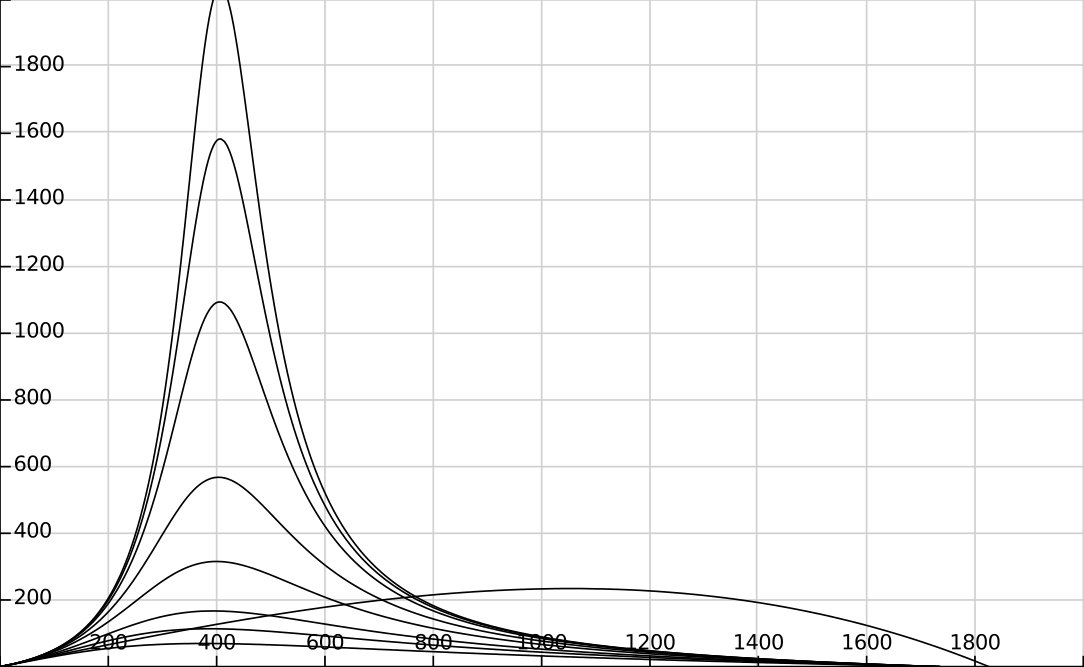 Figure 1
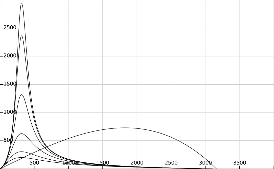 Figure 2
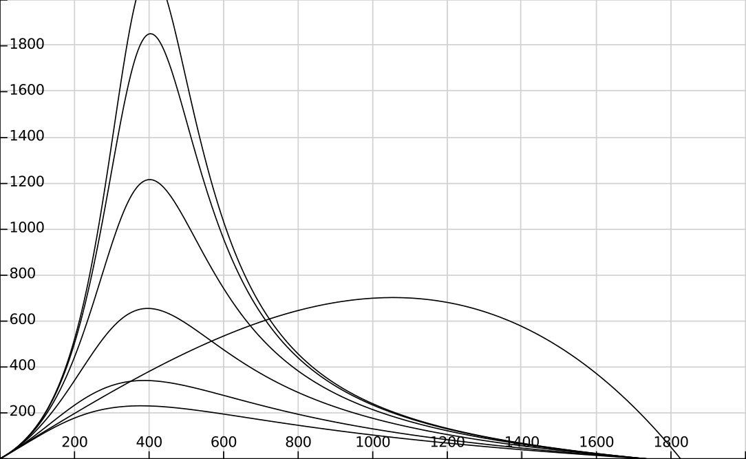 Figure 3
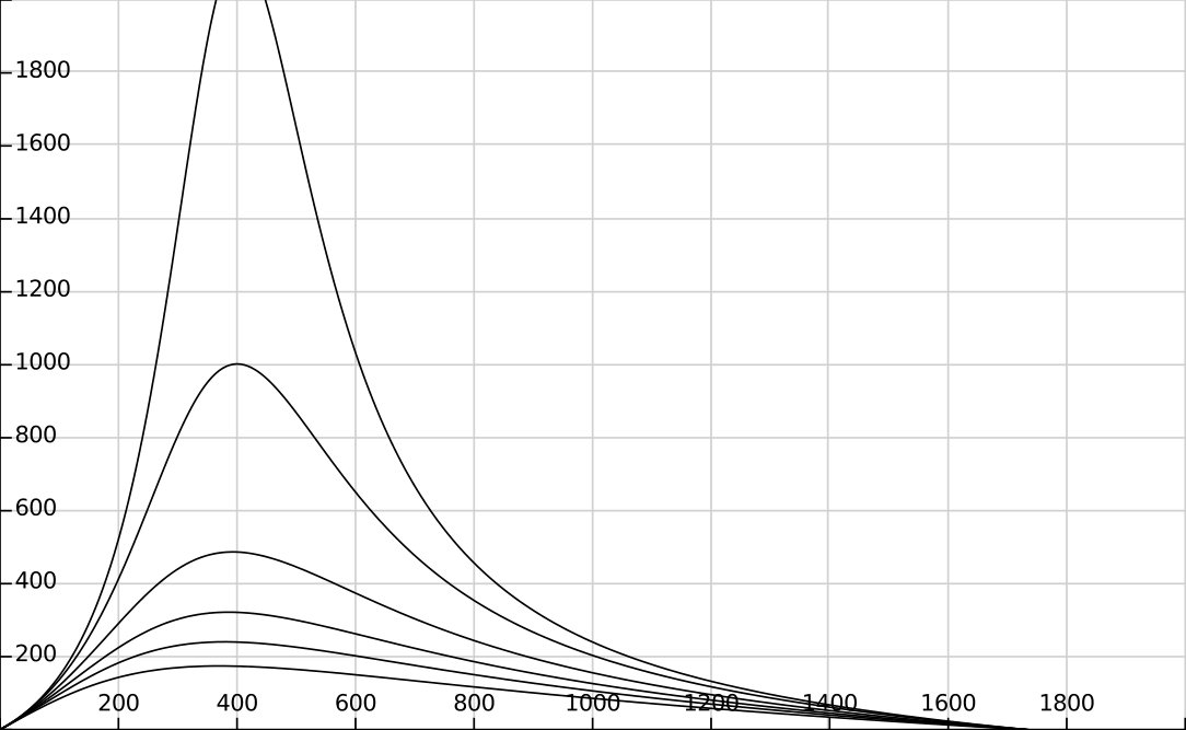 Figure 4
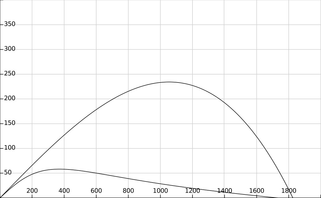 Figure 5
Peer Reviews
No public reviews on file for this paper yet. If you reviewed it on a platform where reviews are public (OpenReview, ICLR, NeurIPS, ICML), you can paste yours below so the community can read it here.
Videos
No videos yet. Explain this paper in a talk, walkthrough, or lecture? Add one.
On the displacement of two immiscible Oldroyd-B fluids in a Hele-Shaw cell
Gelu I. Paşa, Simion Stoilow Institute of Mathematics of Romanian Academy,
P.O. BOX 1-764, RO-14700, Bucharest, Romania
Abstract. The Saffman-Taylor instability occurs when a Stokes fluid is displaced by a less viscous one in a Hele-Shaw cell. This model is useful to study the secondary oil recovery from a pororus medum. Since 1960, polymer solutions were used as displacing fluids; moreover, the oil in a porous reservoir can often be considered a non-Newtonian fluid. Motivated by this fact, in this paper we study the linear stability of the displacement of two Oldroyd-B fluids in a rectilinear Hele-Shaw cell, even if the direct relevance for the flow through porous media is not so evident. We get an approximate formula of the growth rate of perturbations, which depends on the difference of the Weissenberg numbers of the two fluids. A blow-up of the growth rate appears for a critical value of this difference. This singularity is in agreement with previous numerical and experimental results, already reported by several papers concerning the flow of complex fluids in Hele-Shaw cells.
Key words: Hele-Shaw immisible displacement; Oldroyd-B fluids; linear stability; growth rate formulas.
1 Introduction
A Hele-Shaw cell is a technical device introduced in [16], formed by two parallel plates separated by a narrow gap. The equations verified by the mean velocities of a Stokes fluid in a Hele-Shaw cell are similar with the Darcy’s law for flow in a porous medium - see [2], [18]. The interface between two immiscible Stokes fluids in a Hele-Shaw cell is unstable when the displacing fluid is less viscous - see Saffman and Taylor [31].
The Hele-Shaw model can be used to study the secondary oil recovery. Since 1960, good results were obtained by using a polymer solution as ”forerunner” in the oil recovery process - see [12] and the references therein. The oil can often be considered a non-Newtonian fluid, so it is useful to study the stability of the non-Newtonian displacements in Hele-Shaw cells.
The non-Newtonian fluids are studied in a large number of papers - see [4], [11], [13], [23], [29], [32], [33]. This fluids exhibit at least two characteristics not present in Newtonian case: shear-thinning and elasticity. Two important constitutive models exists in order to describe these effects. The Ostwald-de Waele power-law fluid shows shear-thinning but is inelastic. The Oldroyd-B model exhibits elasticity but not shear-thinning.
Important results about the stability of non-Newtonian displacements in Hele-Shaw cells were obtained in [1], [3], [9], [20], [21], [30], [35].
A formula of the growth rate of perturbations was obtained in [35], when a power-law fluid (with exponent ) is displaced by air in a rectiliniar cell. It is multiplied by as compared with the Newtonian case, but there is no qualitative change.
In [1] is studied the flow near an arbitrary corner for any power-law fluid. The variational calculus is used in [3], to investigate the time-dependent injection rate that minimises the Saffman -Taylor instability, when shear-thinning fluids, slowly gelling or fast gelling polymer solutions are displacing. In [9] are studied some methods for minimize the fingering phenomenon when an inviscid fluid displaces a power-law fluid. The problem of bubble contraction in a Hele-Shaw cell is studied in [20], when the surrounding fluid is of power-law type, related with a small perturbation of the radially symmetric problem. The stability of the displacement of two power-law fluids in a radial Hele-Shaw cell has been considered in [21]. The displacement of a high-viscosity power-law fluid by a low-viscosity Newtonian fluid in a radial Hele-Shaw cell is studied in [30] and a detailed analysis of the flow is given, concerning the fractal fingering patterns.
Numerical results concerning the displacement of Oldroyd-B and Maxwell upper - convected fluids by air in rectilinear Hele-Shaw cells are given in [24], [25], [35]. A blow-up of the growth constant was reported in [35], when the relaxation (time) constant is increasing up to a critical value. This phenomenon may be related with the fractures observed in the flows of complex fluids in Hele-Shaw cells - see [26], [27], [36] and the references therein.
In this paper we study the linear instability of the displacement of two Oldroyd-B fluids in a rectilinear Hele-Shaw cell. We use the same depth-averaged interface conditions as in [31], [35]. The thickness of the narrow gap is much smaller compared with the cell lenght, then we can neglect some terms in the perturbations equations. The new element is the explicit formula (56) of the growth rate of perturbations, obtained in terms of , where are the Weissenberg numbers of the two fluids. Most numerical methods fail when the Weisenberg numbers are near 1. A blow-up of our growth rate formula (56) appears for some critical values . Therefore the instability is due to the model.
The paper is organized as follows. In section 2 we describe the Hele-Shaw cell and the constitutive equations of the Oldroyd-B fluids. The basic solution is given in section 3. In section 4 we get the linear perturbation system. The stability analysis is performed in section 5. A special Fourier decomposition used in section 5.1 allows us to avoid the unbounded growth of the partial derivatives of the perturbed velocity near the interface between the two fluids. In section 5.2 we get the leading order terms of the extra-stress tensor and the amplitude of the velocity perturbations. In section 6 we obtain the growth rate formula. In section 7 we give new rezults on the effects of superficial tension in the stability of the displacement process. Some dispersion curves are plotted, in good agreement with previous numerical results. We conclude in section 8. The calculations and complex formulas required for exposure are detailed in Appendix 1-3.
2 The Oldroyd-B fluids
We consider two incompressible immisicble Oldroyd-B fluids in a Hele-Shaw cell parallel with the plane. The cell plates are separated by a gap of thickness . The cell length is denoted by and we use the small parameter
[TABLE]
The fluid 1 is displacing the fluid 2 in the positive direction of the axis. Across the sharp interface bewteen the fluids, the jump of the averaged normal stress should equal the surface tension times the curvature of averaged interface and the normal velocity should be continuous (the ”depth-averaged” Laplace’s law). The no-slip conditions are imposed on the cell plates.
The velocities, the pressures, the viscosities and the extra - stress tensors for both fluids are denoted by
[TABLE]
The stress and the strain-rate are given by
[TABLE]
[TABLE]
[TABLE]
where is the unit tensor and is the gradient operator.
We have the following flow equations, divergence-free condition and constitutive relations, with :
[TABLE]
[TABLE]
[TABLE]
[TABLE]
Here are the relaxation and the retardation (time) constants of the fluids. The lower indexes x, y, z are denoting the partial derivatives; are the upper convected derivatives. We consider a steady flow, then
[TABLE]
[TABLE]
3 The basic flow
We study the linear stability of the following basic flow, denoted by the super index 0i, :
[TABLE]
[TABLE]
[TABLE]
The basic extra-stress tensor (depending only on ) is given by the equations (74) - (76) in Appendix 1 and it follows (see also [35]):
[TABLE]
[TABLE]
Therefore we obtain the following basic flow equations
[TABLE]
[TABLE]
From the relation we get
[TABLE]
where are two negative constants. We suppose for , then we obtain
[TABLE]
The normal velocity must be continuous across the interface. Our basic velocity has only the normal component, then and we have the important relation
[TABLE]
*The basic flow velocity * is given by
[TABLE]
We define the average operator
[TABLE]
and we introduce the characteristic velocity :
[TABLE]
The relation (15) is similar with the Darcy’s law for a porous medium with permeability .
We consider the following basic interface between the displacing fluids
[TABLE]
where is time and we introduce the moving reference
[TABLE]
Then the basic (material) steady interface becomes
[TABLE]
In the following we still use the notation instead of .
It is noteworthy that in [35] is considered the planar interface , by using the relation (15). In [25], after the formula (10), it is specified that “since is much smaller than any lateral lengthscale in a Hele-Shaw device, then any dependence of the basic interface is not relevant”.
The flow is due to the pressure gradients. The pressures contain two unknown constants, used latter in order to obtain the Laplace’s law for perturbations.
4 The perturbations system
The linear perturbations of the basic solution (6) are denoted by
[TABLE]
We assume for . The perturbation of the basic interface (18) is denoted by and we have
[TABLE]
The basic velocities verify the divergence-free relation. In the frame of linear perturbations we obtain . We use the average operator (14) and get
[TABLE]
This condition is verified if , from which we get . In this paper we consider
[TABLE]
The following relations (21) - (26) are concerning both fluids 1 and 2, then we omit the super index i. We introduce the small perturbations in (3)-(5) and obtain
[TABLE]
[TABLE]
[TABLE]
[TABLE]
[TABLE]
[TABLE]
where verify the relations
[TABLE]
[TABLE]
In the frame of the linear stability (by neglecting the second order terms in perturbations) it follows
[TABLE]
where the tensors are given in Appendix 2 - see the relations (77)-(79).
The perturbed normal stresses in both fluids are given by (see [29], [5])
[TABLE]
We search for the limit values and .
The basic pressure is not depending on , then we have the following first order expansion near the basic interface :
[TABLE]
[TABLE]
Recall (19), then is continuous across the interface and we get
[TABLE]
[TABLE]
The depth-averaged dynamic Laplace’s law (near the basic interface ) is
[TABLE]
where is the surface tension. From (27), (28) it follows
[TABLE]
[TABLE]
[TABLE]
where the curvature of is approximated by . The basic normal stress verify the Laplace’s law on the basic interface , so we should have the relationship
[TABLE]
[TABLE]
Only the basic pressures gradients are given, then the basic pressures contain two additive constants. As in [35] (where the displacing fluid is air), for appropriate values of these constants we get the above relation - see also the last two lines of section (4). Therefore the relations (29)-(30) are giving us the Laplace’s law for perturbations:
[TABLE]
[TABLE]
5 Linear stability analysis
5.1 Fourier decomposition
We consider the following expansions of the velocity perturbations, with :
[TABLE]
[TABLE]
[TABLE]
[TABLE]
[TABLE]
[TABLE]
[TABLE]
The dimension of is length. On we have
[TABLE]
[TABLE]
[TABLE]
where are the lateral limits values. The perturbations decay to zero far from the interface and in both fluids. If , then near are bounded in terms of . We justify the form of the amplitude in section 5.2.
The perturbation of the basic interface was denoted by - see (19). The Fourier decomposition (32)-(35) gives us and from (31) it follows
[TABLE]
where . We have to obtain as a functions of basic and perturbed velocities. In this paper we use the following dimensionless quantities, denoted by ′ :
[TABLE]
[TABLE]
[TABLE]
[TABLE]
[TABLE]
[TABLE]
[TABLE]
Here are the Weissenberg numbers. We consider that are of order .
5.2 Leading order terms for
In this subsection we use only the dimensionless quantities, but we omit the ′. We obtain approximate formulas of in terms of .
The leading order expressions for all components of are given in Appendix 3. For both fluids () we have
[TABLE]
[TABLE]
[TABLE]
We get by using the flow equations and the divergence-free condition:
[TABLE]
[TABLE]
[TABLE]
[TABLE]
We also have and from (43) it follows
[TABLE]
On the same way we get
[TABLE]
As , from (44) - (45) we obtain
[TABLE]
The form of the amplitude is justified as follows. From (42), (44) we should have
[TABLE]
We prove that . For this, we recall and we use the inequality
[TABLE]
[TABLE]
which holds for and . Then
[TABLE]
The decomposition (32)-(35) is giving us . Then verifies (47) with the precision order , if is large enough.
6 The growth rate formula
In this section we use both dimensional and dimensionless quantities (the last are denoted by ) and obtain the growth-rate formula. The flow equations ad the decomposition (32)-(35) give us
[TABLE]
[TABLE]
The dimensional forms of the equations (88), (99) in Appendix 3 are
[TABLE]
[TABLE]
The relations (32), (33), (36) and (48) - (49) give us
[TABLE]
[TABLE]
[TABLE]
[TABLE]
[TABLE]
[TABLE]
We use (31), (50), (51) and we get
[TABLE]
[TABLE]
[TABLE]
[TABLE]
[TABLE]
From (11) - (15) we obtain the following averages
[TABLE]
[TABLE]
[TABLE]
then leads us to:
[TABLE]
Let be the capillary number, then the relation (53) becomes
[TABLE]
The dimensional Saffman-Taylor formula is
[TABLE]
When we have the same numerators in (54) and (55); only the denominator of (54) contains the two new terms instead of .
From (38), (52), (53) and (55) we get the dimensionless expressions
[TABLE]
[TABLE]
Remark 1. We have
[TABLE]
[TABLE]
Then, near the basic interface, given by (27) is depending on . But our basic pressures must depend only on - see (9). We can partially overcome this inconsistency by using the parameter . For this, we estimate the partial derivative of the perturbed interface with respect to . As we mentioned at the end of section 5.1, we consider . Then we have
[TABLE]
[TABLE]
A large enough is giving us an arbitrary small . If in the decomposition (32)-(35), then for and we get .
Remark 2. Our model can describe the displacement of an Oldroyd-B fluid by air. For this, we consider (12) in the form . As the displacing fluid is air, then and from (12), (48), (49) we get
[TABLE]
In this case the Laplace’s law (31) becomes
[TABLE]
This form of the Laplace’s law (by neglecting the meniscus curvature ) was used in [35], based on the additional hypothesis
[TABLE]
which in fact it’s not necessary. If then the formula (53) becomes
[TABLE]
In we put . Moreover, . Then we get the dimensionless growth rate
[TABLE]
The dimensionless Saffman-Taylor formula is
[TABLE]
7 Discussions and results
A. We consider . Then the growth constant (56) becomes
[TABLE]
therefore . Two new terms appear in (63), compared with the formula (57):
i) in the denominator; ii) in the numerator.
The dispersion curves are given in Figure 1. The new terms in the formula (63) appear from two reasons:
a) we not neglected in front of ;
b) we used the total curvature of the perturbed interface in the Laplace law (31).
As a consequence, we obtain the following results:
A1) Even if the surface tension on the interface is zero, the growth constant is bounded in terms of the wave number . The equation (63) with gives us
[TABLE]
[TABLE]
Indeed, we have
[TABLE]
[TABLE]
A2) If the surface tension on the interface is zero, then the growth constant tends to zero for very large wave numbers .
We cite here some results obtained for displacements of immiscible Newtonian fluids with very small (or zero) surface tensions on the intrerface, in 2D Hele-Shaw cells.In [34] (Introduction) it is specified that ”One asks whether a non-zero-surface-tension model approximates the zero-surface-tension one. The answer is negative in the case of a receding fluid (see numerical evidence in [8], [28]). In the case of injection the answer is supposed to be affirmative but is still unknown”. In [19] is given a perturbation theorem for strong polynomial solutions to the zero surface tension Hele-Shaw equation driven by injection or suction, the so called Polubarinova - Galin equation. In the case of suction, by using some additional hypothesis, it is proved that the most part of the fluid will be sucked before the strong solution blows up.
The above results A1) and A2) are in contradiction with the Saffman-Taylor formula (57), where is giving an unbounded growth constant in terms of .
A3) From (63) we get
[TABLE]
and it follows
[TABLE]
The growth constant is negative or zero when the surface tension is large enough, even if the displacing fluid is less viscous (that means ). This is also in contradiction with the Saffman-Talor criterion derived from (55). This is an important result of our paper: the displacement stability in a 3D Hele-Shaw cell is decided not only by the ratio of the viscosities of the two fluids, but also by the surface tension on the interface. When the displacing fluid is less viscous, the sufficient condition for the almost stability is
[TABLE]
A quite similar result is given by the formula (19) of [22]: the growth-rate can not be positive for large enough surface tension. But in our formula (67) we have also the viscosities ratio.
A different contradiction of the Saffman and Taylor stability criterion was observed in [6], [7], [10], [14], [15], [17]. All these papers are related with the displacement of air (then is almost zero) by a fluid with surfactant properties in a Hele - Shaw cell with preexisting surfactant layers on the plates; it is pointed out that a more viscous displacing fluid can give us an unstable air-fluid interface. The experiments and the numerical results are in good agreement - but also in a 3D frame. We can consider that our result is a complementary one, compared with the above experiments with surfactants fluids and Hele-Shaw cells. We proved that for a large enough surface tension, even if the displacing fluid is less viscous, the interface air-fluid is almost stable.
B. Consider now the case when at least one of the Weissenberg numbers is not equal to zero and .
B1) Let . We use the notations (52) and introduce the new quantity :
[TABLE]
In the formula (56) we must avoid the critical value
[TABLE]
The denominator of the growth rate (56) is strictly positive in the range . As a consequence, from (56) we get the following instability criterion:
[TABLE]
[TABLE]
Moreover, when
[TABLE]
the denominator of (56) is close to zero and we get a blow-up of the growth rate. Then a strong destabilizing effect appears, compared with the case of Newtonian displacing fluids.
We have also
[TABLE]
[TABLE]
B2) If and or we have a Stokes displacing fluid. In this case, with we recover the above results (70) - (71).
We consider a Stokes fluid (so ) displacing an Oldroyd-B fluid with the Weissenberg numbers . In Figures 2,3 we compare our dispersion curves (56) and Saffman-Taylor formula (57), in the case , for and . The maximum value of given by (56) is increasing as function of until the blow-up appears, for a finite value of which we denote by . The formula (69) gives us
[TABLE]
If the ratio is increasing, then the critical numbers for which the blow-up of the growth rate appears is decreasing. For we get . This is natural: if the viscosity of the displacing fluid is decreasing to zero then the blow-up of appears ”earlier”, for smaller values of .
In Figures 4, 5 are plotted the growth rates (61) when air (then ) is displacing an Oldroyd-B fluid. In Figure 4 we compare (61) and (62) for . The maximum value of is increasing in terms of until we get the blow-up of the growth rate for the critical value
[TABLE]
In Figure 5 are plotted the growth rates (61) when and , for = 1, 0.7, 0.5, 0.3, 0.1, 0. The dispersion curves given in Figures 4,5 are quite similar with the numerical results given in Figures 1, 3 of [35].
8 Conclusions
In the last decades, some important results were established concerning the linear stability of the displacement of immiscible non-Newtonian fluids in Hele-Shaw cells.
The displacement of a power-law fluid by air in a rectilinear cell was studied by Wilson [35] and a formula of the growth rate of perturbations was given, but there is no qualitative change compared with the Saffman-Taylor result. The case of radial displacements is different and was studied in subsequent papers; the effect of the interfacial tension was highlighted.
Numerical results were obtained concerning the displacement of an Oldroyd-B fluid by air in rectilinear cells. A blow-up of the numerical growth rate was reported, in accord with some experimental results concerning the flow of complex fluids in Hele-Shaw cells. On the other hand, most numerical methods shows the existence of a critical value of the Weissenberg numbers beyond which no discrete solutions can be obtained.
In this paper we study the linear instability of the steady displacement of two Oldroyd-B fluids in a rectilinear Hele-Shaw cell. We use the Fourier decomposition (34) for the velocities and obtain the formula (56) of the growth rate of disturbances, which presents a blow-up for some critical values of the Weissenberg numbers.
In the case of two Newtonian displacing fluids, our growth rate is less than the Saffman-Taylor value, but no qualitative change appears - see Figure 1. We prove that the flow stability is decided not only by the ratio of the displacing fluids viscosities, but also by the surface tension on the interface - see the relations (65) - (67). The Saffman - Taylor viscous fingering problem in rectangular geometry is studied in [22], highlighting the link between interface asymmetry and viscosity contrast. The equation (19) of [22] shows that the growth rates will not become positive if the surface tension is large enough. This is in agreement with our result A3) in section 7.
In the case of two Oldroyd-B displacing fluids we get the instability criterion (70). A strong destabilization effect appears, compared with the Newtonian displacements. The dispersion curves when the displacing fluid is Stokes (or air) are plotted in Figures 2-5. Our analytical results are quite similar with numerical results already obtained in [35], then the instability is due to the flow model, at least for the flow geometry considered here.
**Appendix 1 - the equations of the basic extra-stress tensors . **
The basic extra-stress tensors in both fluids are obtained from (3) - (6):
[TABLE]
[TABLE]
[TABLE]
[TABLE]
[TABLE]
[TABLE]
[TABLE]
[TABLE]
[TABLE]
[TABLE]
**Appendix 2 - the tensors E, F, S in the formula (26). **
[TABLE]
[TABLE]
[TABLE]
[TABLE]
[TABLE]
[TABLE]
[TABLE]
[TABLE]
[TABLE]
[TABLE]
[TABLE]
[TABLE]
**Appendix 3 - the extra-stress perturbations . **
[TABLE]
[TABLE]
[TABLE]
[TABLE]
[TABLE]
At the leading order, from (80) we get
[TABLE]
The partial derivatives near are bounded in terms of , due to the Fourier decomposition (32) - (35) with . Moreover, we have
[TABLE]
then from the relations (81) - (84) it follows
[TABLE]
[TABLE]
The dimensionless form of is , therefore from the last relations it follows
[TABLE]
[TABLE]
We use again (84) and relations (86) lead us to
[TABLE]
In (80) - (87) replace by , then for we obtain
[TABLE]
- The dimensionless form of the relations (26) gives us the component of in the fluid 1 (in the formulas (89) - (92) below we omit the upper index 1):
[TABLE]
[TABLE]
[TABLE]
We suppose
[TABLE]
We insert the expression (90) in the equation (89) and get
[TABLE]
[TABLE]
[TABLE]
The Fourier decomposition (32) gives us
[TABLE]
Then the formula (90) is verified if we can neglect the term in front of the first two terms appearing in the equation (91). We recall that are bounded with respect to , then
[TABLE]
[TABLE]
[TABLE]
We neglect the term of order in the equation (91) and obtain the approximate formula
[TABLE]
in agreement with the hypothesis (90).
On the same way we get the approximate formula of in the second fluid:
[TABLE]
We emphasize that appear in the approximate curvature of , so they can not be neglected.
- The dimensionless form of the relations (26) gives us the component of in the fluid 1 (in the formulas (95) - (98) below we omit the index 1):
[TABLE]
[TABLE]
[TABLE]
We suppose
[TABLE]
We introduce the expression (96) in (95) and get
[TABLE]
[TABLE]
[TABLE]
The Fourier decomposition (32) gives us
[TABLE]
If we get
[TABLE]
[TABLE]
[TABLE]
We neglect the term of order in the equation (97) and get the formula (96). Therefore, for , we have
[TABLE]
- The dimensionless constitutive relation for is
[TABLE]
and at the leading order we get
[TABLE]
The reference list from the paper itself. Each links out to its DOI / PubMed record.
- 1[1] G. Aronsson G and U. Janfalk, On Hele-Shaw flow of power-law fluids, Eur. J. Appl. Math. 3 (1992), 343–66.
- 2[2] J. Bear, Dynamics of Fluids in Porous Media, Elsevier, New York, 1972.
- 3[3] T. H. Beeson-Jones and A. W. Woods, Control of viscous instability by variation of injection rate in a fluid with time-dependent rheology, J. Fluid Mechanics 829 (2017), 214-235.
- 4[4] R. B. Bird, W. E. Stewart, E. N. , Transport phenomena, Vol. 1: Fluid Mechanics, John Wiley and Sons, N Y, 1960.
- 5[5] J. M. Bush, Surface Tension Module, Lect. Notes, MIT, 2013.
- 6[6] C. K. Chan and N. Y. Liang, Observation of surfactant driven instability in a hele-Shaw cell, Phys. Rev. Lett. 79 (1997), 4381-4384.
- 7[7] C. K. Chan, Surfactant wetting layer driven instability in a Hele-Shaw cell, Physica A, 288 (2000), 315-325.
- 8[8] H. G. Ceniceros, T. Y. Hou and H. Si, Numerical study of Hele–Shaw flow with suction, Phys. Fluids 11 (1999), 2471–2486.