On a class of linear functional equations without range condition
Eszter Gselmann, Gergely Kiss, Csaba Vincze

TL;DR
This paper characterizes all solutions to a broad class of linear functional equations involving sums over fixed coefficients, providing explicit descriptions and conditions for non-trivial solutions in linear spaces.
Contribution
It offers a comprehensive solution framework for a class of linear functional equations without range restrictions, including necessary and sufficient conditions for non-trivial solutions.
Findings
Explicit general solutions for the functional equations
Necessary and sufficient conditions for non-trivial solutions
Framework applicable to linear spaces over any field
Abstract
The main purpose of this work is to provide the general solutions of a class of linear functional equations. Let be an arbitrarily fixed integer, let further and be linear spaces over the field and let , be arbitrarily fixed constants. We will describe all those functions , that fulfill functional equation \[ f\left(\sum_{i=1}^n \alpha_i x_i, \sum_{i=1}^n \beta_i y_i\right)= \sum_{i, j=1}^{n}f_{i, j}(x_i, y_j) \qquad \left(x_i \in X, y_i \in Y, i=1, \ldots, n\right). \] Additionally, necessary and sufficient conditions will also be given that guarantee the solutions to be non-trivial.
Click any figure to enlarge with its caption.
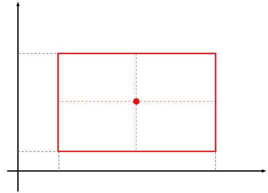 Figure 1
Peer Reviews
No public reviews on file for this paper yet. If you reviewed it on a platform where reviews are public (OpenReview, ICLR, NeurIPS, ICML), you can paste yours below so the community can read it here.
Videos
No videos yet. Explain this paper in a talk, walkthrough, or lecture? Add one.
On a class of linear functional equations
without range condition
Eszter Gselmann, Gergely Kiss and Csaba Vincze
Abstract
The main purpose of this work is to provide the general solutions of a class of linear functional equations. Let be an arbitrarily fixed integer, let further and be linear spaces over the field and let , be arbitrarily fixed constants. We will describe all those functions , that fulfill functional equation
[TABLE]
Additionally, necessary and sufficient conditions will also be given that guarantee the solutions to be non-trivial.
Dedicated to Professor János Aczél on the occasion of his th birthday. *
1 Introduction
As János Aczél wrote in his famous and pioneering monograph [1]: ‘Functional equations have a long history and occur almost everywhere. Their influence and applications can be felt in every field, and all fields benefit from their contact, use, and technique.’ Almost the same can be said about the class of linear functional equations. This area is one of the most investigated topic in this field, several authors studied this class, see e.g. [2, 3, 4, 5, 6, 7, 8, 9, 10, 14, 18, 19, 20].
The main purpose of this paper is to describe the general solutions of a class of linear functional equations. More precisely, we are interested in the following problem. Let be an arbitrarily fixed integer, let further and be linear spaces over the field and let , be arbitrarily fixed constants. Assume further that for the functions , , functional equation
[TABLE]
is fulfilled.
This equation belongs to the class of linear functional equations, that was thoroughly investigated by L. Székelyhidi in [15, 16, 17]. For the sake of completeness, here we briefly recall the main results from Székelyhidi [15].
Definition 1**.**
If are groups and is a positive integer, then a function is said to be -additive if it is a homomorphism in each variable. Let be a function, then the function defined by
[TABLE]
is said to be the diagonal of and it is denoted by . Further, let
[TABLE]
Remark*.*
Let be groups, be a positive integer and be an -additive function. Then for all and for arbitrary we have
[TABLE]
For a function , denotes the range of .
Definition 2**.**
Let be Abelian groups, let be a non-negative integer. The function is said to be of degree , if there exist functions and homomorphisms such that
[TABLE]
and functional equation
[TABLE]
holds.
Definition 3**.**
Let be Abelian groups, let be a non-negative integer. The function is called a (generalized) polynomial degree , if for all there exists a -additive mapping such that
[TABLE]
where [math]-additive functions are to be understood constant functions.
Theorem 1** (Theorem 3.6 of [15]).**
Let be Abelian groups and suppose that is divisible. Let be a non-negative integer. The function is of degree if and only if it is a polynomial of degree .
Theorem 2** (Theorem 3.9 of [15]).**
Let be Abelian groups and suppose that is divisible and is torsion free. Let be a non-negative integer and let be homomorphisms of onto itself such that
[TABLE]
The functions satisfy functional equation
[TABLE]
if and only if for all and there exist symmetric -additive functions such that
[TABLE]
and the equations
[TABLE]
hold for all and .
Observe that equation (1) can be reduced to the form (1). Indeed, suppose that (or substitute zero in place of the variables except a distinguished pair) and consider the following family of homomorphisms
[TABLE]
With these notations (1) can be re-written as
[TABLE]
At the same time (as it can be seen in the following subsection), we cannot state that the functions involved are polynomials. This is because the fact that the homomorphisms defined above in general do not fulfill range condition , neither fulfill range condition . What is more, they are injective if and only if and in such a situation . Notice that equation (1) involves the projections and . None of these are injective. This shows that Theorems 1 and 2 cannot be applied in our situation.
2 Special cases of the original equation
2.1 The one-variable sub-case
In this sub-case let be arbitrarily fixed, be a linear space over the field and suppose that for the functions functional equation
[TABLE]
holds with certain constants .
Observe that without loss of generality
[TABLE]
can be assumed. Otherwise we consider the functions
[TABLE]
They clearly vanish at zero and they also fulfill the above functional equation. Therefore from now on we always suppose that holds.
As we will see, the solutions of equation (1) heavily depend on whether or not there are zeros among the parameters . We may (and also do) assume that these parameters are arranged in the following way: there exists a non-negative integer such that for , but for all .
Proposition 1**.**
Let be arbitrarily fixed, be a linear space over the field and suppose that for the functions functional equation (1) holds with certain constants and assume that is also satisfied. Suppose further that for , but for all . Then
- (i)
in case , all the functions are identically zero and is any function fulfilling , 2. (ii)
in case , all the functions are identically zero and are any functions vanishing at zero and fulfilling
[TABLE] 3. (iii)
otherwise, there exists an additive function such that
[TABLE]
and the functions are identically zero.
Conversely, the mappings vanish at zero and they also fulfill (1).
Proof.
In case equation (1) reduces to
[TABLE]
Since we have independent variables, this immediately yields that the involved functions have to be constant functions. In view of this means that they have to be identically zero and the only information we get for the function is that .
In case , our equation can be written as
[TABLE]
With the substitution
[TABLE]
we obtain that
[TABLE]
which (similarly as above) yields that the functions are identically zero. Using this, the functions fulfill
[TABLE]
If , this is nothing but
[TABLE]
showing that in this case there is nothing to prove.
Assume that and let be different integers. Then equation (1) with for is
[TABLE]
which, after introducing the functions
[TABLE]
can be reduced to the system of Pexider equations
[TABLE]
This means that there exists an additive function such that
[TABLE]
∎
3 The two-variable case with
In this section we will focus on functional equation
[TABLE]
where denote the unknown functions and are given constants.
Observe that without loss of generality
[TABLE]
can be supposed. Otherwise we consider the functions
[TABLE]
They clearly vanish at the point and they also fulfill the same functional equation. Similarly as previously, from now on we always suppose that all the involved functions vanish at the point .
This section will be divided into two parts. At the first one, we will consider the so-called degenerate cases, where at least one of the parameters is zero. After that the non-degenerate case will follow, that is, when none of the above parameters are zero.
3.1 Degenerate cases
3.1.1 The homogeneous case
In case equation (2) reduces to
[TABLE]
Proposition 2**.**
Let and be linear spaces over the field and be functions such that
[TABLE]
Then and only then for all there exist functions and vanishing at [math] such that
[TABLE]
as well as
[TABLE]
Proof.
For let us define the functions and through
[TABLE]
With the notation
[TABLE]
identities
[TABLE]
give that
[TABLE]
Moreover, equations
[TABLE]
yield that
[TABLE]
where we used the previously proved identities, too. ∎
3.1.2 The case and
In such a situation (2) reduces to
[TABLE]
Obviously, can be assumed, otherwise we consider the functions defined through
[TABLE]
Proposition 3**.**
Let and be linear spaces over the field and be functions such that
[TABLE]
Then and only then for all there exist functions and vanishing at [math] such that
[TABLE]
as well as
[TABLE]
Proof.
For let us define the functions and through
[TABLE]
Furthermore, let
[TABLE]
to obtain the following system of equations
[TABLE]
or equivalently
[TABLE]
Finally, the system of equations
[TABLE]
yields that
[TABLE]
which in view of the above definitions completes the proof. ∎
3.1.3 The case and
In such a situation (2) implies that
[TABLE]
because the left hand side does not depend on and .
Obviously, can be assumed, otherwise we consider the functions defined through
[TABLE]
Proposition 4**.**
Let and be linear spaces over the field and be functions such that
[TABLE]
Then and only then there exists an additive function such that
[TABLE]
Proof.
Consider the functions defined through
[TABLE]
to get the following Pexider equation
[TABLE]
Since all the functions vanish at zero, we get that and the function has to be additive. ∎
To finish the discussion of equation (2) in this special case, apply Proposition 2 to the functions
[TABLE]
where are given in Proposition 4.
3.1.4 The case and
In such a situation (2) implies that
[TABLE]
because the left hand side does not depend on and .
Obviously, due to similar reasons as previously, can be assumed. The proof of the following proposition is a straightforward calculation, so we omit it.
Proposition 5**.**
Let and be linear spaces over the field and be functions. Functional equation
[TABLE]
is fulfilled if and only if there exist functions and such that
[TABLE]
To finish the discussion of equation (2) in this special case, apply Proposition 2 to the functions
[TABLE]
where and were determined in Proposition 5.
3.1.5 The case and
In such a situation (2) implies that
[TABLE]
because the left hand side does not depend on .
Obviously, due to similar reasons as previously, can be assumed.
Proposition 6**.**
Let and be linear spaces over the field and be functions. Functional equation
[TABLE]
is fulfilled if and only if there exist a mapping additive in its first variable and there are functions and vanishing at zero so that is additive and
[TABLE]
and also
[TABLE]
hold.
Proof.
With the substitution our equation yields that
[TABLE]
From this we immediately get that
[TABLE]
where the functions are defined by
[TABLE]
This means that the functions fulfill a Pexider equation on for any fixed . Thus there exists a mapping additive in its first variable and functions so that
[TABLE]
and
[TABLE]
In terms of the functions this means that
[TABLE]
where
[TABLE]
Observe that is additive. Indeed, using the above the forms of and , our equation with and the fact that is additive in its first variable, we obtain that
[TABLE]
that is, fulfills a Pexider equation. Since , this means that has to be additive. Thus, using again the form of the functions and our equation with , we get that
[TABLE]
Similarly, our equation with implies that
[TABLE]
∎
To finish the discussion of equation (2) in this special case, apply Proposition 2 to the functions
[TABLE]
where and are given in Proposition 6.
3.2 The non-degenerate case
After making clear the degenerate cases, now we can focus on the case and provide the general solution of the functional equation
[TABLE]
where denote the unknown functions and are given constants.
Obviously, it is enough to consider the case , that is, to consider the following functional equation
[TABLE]
In this subsection we always assume that the characteristic of the field is different from .
Proposition 7**.**
Let and be linear spaces over the field . Then the functions satisfy functional equation
[TABLE]
if and only if
[TABLE]
where the mapping is a bi-additive function and for as well as are functions such that and are additive functions and and vanish at the point and
[TABLE]
are also fulfilled.
Proof.
Assume that the functions fulfill functional equation (4) for any and . With the substitution we obtain that
[TABLE]
which immediately implies that
[TABLE]
where the functions are defined by
[TABLE]
This means that there exists a function which is additive in its first variable and a function vanishing at zero such that
[TABLE]
Substituting this form into equation (4), with and with a similar argument we receive that
[TABLE]
where is a bi-additive mapping and is a function that vanishes at zero.
All in all this means that
[TABLE]
Additionally, equation (4), first with yields that has to be additive and secondly, with we receive that the function also has to be additive, too.
Define the functions on through
[TABLE]
to deduce that they fulfill functional equation (3). Due to Proposition 2, for all there exist functions and vanishing at zero such that
[TABLE]
that is, for the functions we have
[TABLE]
Finally, using the equations in Proposition 2 for the functions and , identities
[TABLE]
complete the proof. ∎
3.3 Related equations
3.3.1 The functional equation of bi-additivity
As a trivial consequence of the results of the previous section we get the following.
Corollary 1**.**
Let and be linear spaces over the field with . The mapping fulfills the functional equation of bi-additivity, that is,
[TABLE]
if and only if is bi-additive.
3.3.2 The rectangle equation
Let and be linear spaces over the field and let be a function.
Then functional equation
[TABLE]
or equivalently (provided that )
[TABLE]
is called the rectangle equation.
Indeed, both the above equations express the following: the value of at the center of any rectangle, with parallel sides to the coordinate axes, equals the mean of the values of at the vertices.
y_{2}$$y_{1}$$x_{1}$$x_{2}$$\left(\frac{x_{1}+x_{2}}{2},\frac{y_{1}+y_{2}}{2}\right)$$x$$y
This equation as well as its generalization were investigated (among others) in [2, 5, 14].
With the aid of the results of the previous section, we obtain the following straightaway.
Proposition 8**.**
Let and be linear spaces over the field with and be a function. The function fulfills the rectangle equation, i.e.,
[TABLE]
if and only if there exists a bi-additive mapping and additive functions and such that
[TABLE]
Remark*.*
In case , the rectangle equation reduces to equation
[TABLE]
or equivalently
[TABLE]
Thus, Proposition 2 yields that there exist functions and such that
[TABLE]
The Cauchy equation on
Proposition 9**.**
Let and be linear spaces over the field and be functions. Then functional equation
[TABLE]
holds if and only if there exist additive functions , such that
[TABLE]
4 On the reduction of equations with to the two-variable case
In this section we intend to investigate the following problem. Let and be linear spaces over the field , let further , be arbitrarily fixed constants. Assume further that for the functions , , functional equation
[TABLE]
is fulfilled.
We will show that in case , the results of the previous section can be applied. Indeed, let such that and , but otherwise arbitrary. In this case equation (6) with the substitutions
[TABLE]
yields that
[TABLE]
for any and . Consider the functions defined by
[TABLE]
and
[TABLE]
to receive that
[TABLE]
is satisfied for any and . This equation can however be handled with the aid of the results of Section 3.
5 The case of a single unknown function in the equation — existence of non-trivial solutions
Let and be linear spaces over the same field and consider the following functional equation
[TABLE]
where denotes the unknown function and and are given constants.
Recall that due to the linearity of the above equation we may (and we also do) suppose that
[TABLE]
holds. Otherwise the function
[TABLE]
can be considered. This function clearly vanishes at the point and it fulfills the same functional equation, too.
Furthermore, the linearity of the investigated equation implies that the identically zero function is always a solution. In this section we would like to study under what conditions admits equation (8) a non-identically zero solution. Clearly, in every case the results of the previous sections can be applied with the choice
[TABLE]
This means that the assumption that the function is not identically zero will imply algebraic conditions for the involved parameters and .
Similarly as before, first we consider the so-called degenerate cases.
5.1 Degenerate cases
5.1.1 The case
In case equation (8) reduces to
[TABLE]
where for any .
Proposition 10**.**
Let and be linear spaces over the field , be given constants such that not all of them are zero and be a function such that
[TABLE]
Then and only then there exist functions and vanishing at zero such that
[TABLE]
Furthermore
- (i)
either the following system of linear equations
[TABLE]
is fulfilled or the function is identically zero. 2. (ii)
either the following system of linear equations
[TABLE]
is fulfilled or the function is identically zero.
Proof.
In view of Proposition 2 we get that there exist functions and vanishing at zero such that
[TABLE]
Using this representation of the function , equation (9) yields that
[TABLE]
or equivalently
[TABLE]
Since we have independent variables we get that
[TABLE]
is fulfilled or the function is identically zero. Similarly,
[TABLE]
holds or the function is identically zero. ∎
5.1.2 The case and
In such a situation (8) reduces to
[TABLE]
In view of Proposition 3, the proof of the following proposition is straightforward and similar to that of Proposition 10. The basic step is to consider as the sum of single variable functions (Proposition 3) and substitute such a special form of into the functional equation.
Proposition 11**.**
Let and be linear spaces over the field , be given constants such that not all of them are zero, and be a function such that
[TABLE]
Then and only then there exist functions and vanishing at zero such that
[TABLE]
Furthermore
- (i)
either the following system of linear equations
[TABLE]
is fulfilled or the function is identically zero. 2. (ii)
either the following system of equations
[TABLE]
is fulfilled or the function is identically zero.
5.1.3 The case and
In such a situation (8) reduces to
[TABLE]
As before, taking as the sum of single variable functions (Proposition 4), substitute into the functional equation.
Proposition 12**.**
Let and be linear spaces over the field , be given constants such that not all of them are zero and be a function such that
[TABLE]
Then and only then there exists an additive function and a function vanishing at zero such that
[TABLE]
Furthermore the above additive function has to fulfill
[TABLE]
for arbitrary and for the mapping alternative (ii) of Proposition 10 is fulfilled.
5.1.4 The case and
In such a situation (8) reduces to
[TABLE]
To prove the following result, consider as the sum of single variable functions (Proposition 5) and substitute into the functional equation.
Proposition 13**.**
Let and be linear spaces over the field , be given constants and be a function such that
[TABLE]
Then and only then
- (A)
* and is an arbitrary function fulfilling*
[TABLE] 2. (B)
or there exist functions and vanishing at zero such that
[TABLE]
Furthermore the mappings and also fulfill
[TABLE]
and
- (i)
either
[TABLE]
or is identically zero; 2. (ii)
either
[TABLE]
or is identically zero.
5.1.5 The case and
In such a situation (8) reduces to
[TABLE]
Proposition 14**.**
Let and be linear spaces over the field , , be given constants and be a function such that
[TABLE]
Then and only then there exists a mapping additive in its first variable, further there are functions and vanishing at zero such that is additive and
[TABLE]
Furthermore, we have that
[TABLE]
and also
[TABLE]
yielding that or is identically zero. Additionally, the alternatives below also hold
- A)
either and are zero, that is, equation (13) has the form
[TABLE]
and the identities
[TABLE]
and
[TABLE]
have to hold. 2. B)
or or do not vanish simultaneously and then the mapping has a rather special form, namely there exists an additive function such that
[TABLE]
and therefore
[TABLE]
where the identities
[TABLE]
and
[TABLE]
have to hold.
Proof.
Using Proposition 6 we immediately get that there exists a mapping and there are functions and vanishing at zero such that is additive and
[TABLE]
Using that is additive in its first variable and equation (13) we derive that
[TABLE]
Observe that this equation with implies that
[TABLE]
so or the function is identically zero. Similarly, equation (14) yields with that
[TABLE]
here while proving the last two identities we used that (cf. the proof of Proposition 6) and the fact that for all due to that is additive in its first variable. Put into (14) to receive that
[TABLE]
or in other words,
[TABLE]
Similarly equation (14) with yields that
[TABLE]
or equivalently
[TABLE]
From this latter two identities the following alternatives can be deduced
- A)
either and are zero and equation (13) has the form
[TABLE]
and the identities
[TABLE]
as well as
[TABLE]
follow immediately from (14) with and , respectively. 2. B)
or the two-variable mapping can be represented as
[TABLE]
being additive in its first variable, this is possible if and only if is additive. This means that
[TABLE]
Using this representation and equation (14) first with and after that with we get the identities
[TABLE]
and
[TABLE]
∎
5.2 The non-degenerate case
In view of the above results, now we can focus on the case and investigate the existence of nontrivial solutions of functional equation
[TABLE]
where for , the constants are given.
Here we will make use of the results of Section 3.2, therefore (as in Section 3.2) we always assume that the characteristic of the field is different from . As a direct application of Proposition 7 we derive the following.
Proposition 15**.**
Let and be linear spaces over the field , , be given constants and be a function such that
[TABLE]
Then and only then, there exist a bi-additive function and additive functions and such that
[TABLE]
Furthermore the following identities also have to be fulfilled
[TABLE]
Remark*.*
While investigating whether equation (8) admits or not a non-trivial solution we always got three type of conditions. One of them is a purely algebraic condition, namely we have to check if the parameters fulfill a system of homogeneous, linear equations.
The second type is about the existence of a non-trivial semi-homogeneous additive function. More precisely, this condition is always of the following form: let be a linear space over the field and let be an additive function such that
[TABLE]
with certain fixed scalars . For which values of and will the function be non-trivial (that is, non-identically zero)? This question was firstly investigated in Daróczy [6] if . These results were later generalized and extended in the papers [7, 8, 9, 10, 14, 19, 20]. To the best of our knowledge, this problem has not been investigated in case of fields with nonzero characteristic. To this we provide a solution in Subsection 6.2.
Our third condition is similar to the second one, namely it concerns the non-triviality of a semi-homogeneous bi-additive function. The attached existence problem will also be discussed in the last section.
6 A necessary and sufficient condition for the existence of non-zero, bi-additive semi-homogeneous mappings
According to the characteristic property
[TABLE]
of the bi-additive term in the solution (see Proposition 15), it is natural to investigate the problem of the existence of such non-zero mapping over the field .
Definition 4**.**
Let and be linear spaces over the field . An additive function is called semi-homogeneous if there exist elements , such that
[TABLE]
Similarly, a bi-additive function is called semi-homogeneous if there exist elements , and in the field such that
[TABLE]
6.1 The case of fields with characteristic zero
In this subsection we restrict ourselves to the case of fields with zero characteristic. According to this, let be a field of characteristic zero. Then it is an extension of the field of the rationals and we can consider the subfields and in .
We will also use the following.
Proposition 16**.**
Let be a field of characteristic zero. Then is embeddable into if and only if the transcendence degree of the field extension is less than .
Remark*.*
From the previous proposition we immediately get that if is finitely generated over , that is if , then is embeddable into .
Theorem 3**.**
Let be a field of characteristic zero and suppose that and are linear spaces over . There exists a non-zero bi-additive mapping satisfying (16) if and only if can be written as the product of algebraically conjugated elements to and over , respectively.
Proof.
Suppose that can be written as the product of algebraically conjugated elements to and over , respectively. This means that where and are injective homomorphisms. Taking and as linear spaces over and , respectively, we can write that
[TABLE]
where
- (i)
and are finite index sets such that and , 2. (ii)
, for any , 3. (iii)
, for any , 4. (iv)
belong to a basis of as a linear space over , 5. (v)
belong to a basis of as a linear space over .
The mapping is defined by the formula of the semi-linear extension
[TABLE]
and the values are not all zero.
Conversely, suppose that there exists a non-zero bi-additive mapping satisfying (16). Let us fix elements and such that . Taking the field we can define the bi-additive mapping as
[TABLE]
It can be easily seen that
[TABLE]
is fulfilled for arbitrary .
Let denote the multiplicative subgroup of and let be the group equipped with the pointwise multiplication. Then, for any , the translate mapping, that is,
[TABLE]
also satisfies (17). Let be the set of the restrictions of bi-additive mappings of the form satisfying (17). Then the set is closed with respect to the uniform convergence on finite sets and the field is countable. Therefore is a closed, translation invariant linear space, in other words, it is a variety over a field of finite transcendence degree. From this we infer that spectral analysis holds in , i.e., there exists an exponential element in this variety, see Laczkovich–Székelyhidi [12]. An exponential element in this variety is a bi-additive mapping satisfying (17) such that
[TABLE]
Using the notations and , it follows that where and are injective (field-) homomorphisms of . Using property (17)
[TABLE]
Therefore as it was stated. ∎
6.2 The case of finite fields of non-zero characteristic
If is a field of characteristic different from zero then it is a field of prime characteristic. First of all we collect those results from the theory of finite fields, that we intend to use subsequently. Here we rely on the monograph Lidl–Niederreiter [13]. For any field , there is a minimal subfield, namely the prime field of , which is the smallest subfield containing . It is isomorphic either to (if the characteristic is zero), or to a finite field of prime order (in case ). Moreover, if is a prime and is arbitrary then up to an isomorphism there exists exactly one finite field of order . This field is nothing but the splitting field of the polynomial over . This field is denoted by .
Let now be a semi-homogeneous additive function, that is, assume that for the additive function we have
[TABLE]
As we have seen in the proof of Theorem 3, the problem of the existence of semi-homogeneous mappings defined on the linear space can be reduced to the problem of the existence of semi-homogeneous mappings defined on . It can be easily seen that the additivity automatically implies the homogeneity with respect to the multiplication by the elements of the prime field. By the argument of [18], it also follows that there exists an automorphism between the extensions of the prime field with and , respectively, such that it maps into . Conversely, such an automorphism allows us to use the technique of the semi-linear extension to construct semi-homogeneous additive mappings. This criteria for the existence of semi-homogeneous additive mappings does not depend on the characteristic of the fields but it is worth to investigate the problem of the subfields in in some special cases as follows.
Let be an automorphism of with . Then
[TABLE]
This means that
- (i)
we have to guarantee the existence of an automorphism for which
[TABLE]
is satisfied; 2. (ii)
we have to determine the homogeneity field (see Definition 6) of the additive mapping .
Suppose that for some prime and .
To answer the above questions, for (i) we have to know the automorphism group of , while for (ii) we have to describe the sub-fields of .
Definition 5**.**
Let be a prime and . By an automorphism of over we mean an automorphism of that fixes the elements of . More precisely, we require to be a one-to-one mapping from onto itself with
[TABLE]
and
[TABLE]
Theorem 4**.**
Let be a prime and . The distinct automorphisms of over are exactly the mappings defined by
[TABLE]
Remark*.*
In other words, the above theorem says that the automorphism group of over is a cyclic group of order generated by .
Let be a linear space over the (not necessarily finite) field and be an additive function. Then clearly, for any we have
[TABLE]
Nevertheless, it may happen that satisfies the same identity for all and for some , therefore we introduce the following.
Definition 6**.**
Let be a linear space over the (not necessarily finite) field and be an additive function and
[TABLE]
This set is called the homogeneity field of the additive function . Observe that this term is well-motivated, since we have the following.
Although the following two statements are known in case (see Kuczma [11]), for the sake of completeness we present a short argument for them.
Proposition 17**.**
Let be a linear space over the field and be an additive function. Then is a field.
Proof.
Let , then
[TABLE]
yielding that . Similarly, if , then
[TABLE]
from which follows. ∎
In some sense, the converse is also true, namely we have the proposition below. The proof is based on the existence of Hamel bases of linear spaces. Therefore, in any case it is needed, the Axiom of Choice is supposed to hold.
Proposition 18**.**
Let be a linear space over the field , let further be a subfield of . Then there exists an additive function such that .
Proof.
Let be the Hamel basis of the linear space , which (according to Corollary 4.2.1. of Kuczma [11]) does exist. Fix and define the function by
[TABLE]
Making use of Theorem 4.3.1 of Kuczma [11], there exists a homomorphism from to such that we additionally have that . Clearly, is an additive function and
[TABLE]
Thus .
For the converse statement, let be arbitrary, then , where and for all . Furthermore,
[TABLE]
or equivalently, .
Let now and be arbitrary, then
[TABLE]
On the other hand, since , inclusion implies that there exists such that . Since was to be chosen nonzero, this means that . Therefore . ∎
Theorem 5**.**
Let be a prime and . Then for all , the field admits exactly one subfield isomorphic to and has no other type of sub-fields. Furthermore, this subfield is the set of zeros of the polynomial in .
Finally, we provide necessary and sufficient conditions for the existence of non-zero, bi-additive semi-homogeneous mappings.
The relations among the elements and such that the semi-homogeneity equation (16) is satisfied for some non-zero bi-additive mapping are more implicit as we will see in what follows.
Lemma 1**.**
Let and be linear spaces over the field and let be given non-zero elements. There exists a not identically zero bi-additive mapping satisfying the semi-homogeneity equation (16) if and only if there exists a not identically zero bi-additive mapping satisfying equation
[TABLE]
Proof.
Suppose that satisfies the semi-homogeneity equation (16) and for a certain element . The bi-additive mapping defined by
[TABLE]
obviously satisfies equation (18). Conversely, suppose that satisfies equation (18). Let and be Hamel bases in and , respectively. Taking the projections
[TABLE]
onto the first coordinate of the elements with respect to the given bases it follows that the mapping defined by
[TABLE]
fulfills (16). ∎
Remark*.*
Note that there is no need any additional condition for the cardinality of the field to prove Lemma 1.
From now on the results are strongly based on the cardinality condition for being finite. Let , where for some prime number and consider a (finite) basis of over its prime field . It is clear that
- (H)
bi-additivity implies -homogeneity for any bi-additive mapping .
Since the translation with respect to the multiplication by the th element of the given basis (), that is,
[TABLE]
is a linear transformation, we can consider its matrix representation given by
[TABLE]
where for any possible indices we have . According to property (H), a simple calculation shows that equation (18) is equivalent to
[TABLE]
where , and with .
Let be the linear space of matrices of order over the field and consider the linear mapping
[TABLE]
where
[TABLE]
In a more compact form
[TABLE]
Equation (18) is obviously satisfied if and only if is an eigenvalue of . The corresponding (non-zero) eigenvector can be chosen as the matrix of a bi-linear mapping satisfying (18). To sum up, we can formulate the following result as the answer for the problem of existence of non-identically zero bi-additive mapping satisfying (16).
Theorem 6**.**
Let , where for some prime number and . Consider the polynomial
[TABLE]
where stands for the identity mapping of the linear space of matrices of order over the field . Then the following assertions are equivalent
- (i)
there is a not identically zero bi-additive mapping satisfying the semi-homogeneity equation (18), 2. (ii)
the characteristic polynomial of the linear operator is reducible over the field by one of its non-zero roots, 3. (iii)
**
Remark*.*
If the elements and are given, then the possible ’s are among the roots of the characteristic polynomial . The characteristic polynomial is independent of the choice of the basis . Moreover it is a polynomial over the prime field but the root belongs to in general. Setting the variables and free, the roots of the multivariate polynomial is independent of the choice of the basis . In other words the algebraic variety
[TABLE]
in contains all possible triplets for the solution of the semi-homogeneity equation (16).
6.3 An example: the field
The operations are summarized in the following tables:
[TABLE]
and
[math]
[math] [math] [math] [math] [math]
[math]
[math]
[math]
Since it follows that is a two-dimensional linear space over its prime field . The basis we are going to use in the following is , . An easy computation shows that the translations and are represented by the matrices
[TABLE]
respectively. Choosing elements
[TABLE]
where , it follows that
[TABLE]
where Taking
[TABLE]
a direct computation shows that
[TABLE]
[TABLE]
[TABLE]
[TABLE]
Therefore is represented by the matrix
[TABLE]
with respect to the basis
[TABLE]
If , i.e. and , i.e. , then we have the matrix
[TABLE]
and the characteristic polynomial is
[TABLE]
This means that the possible choices are or , that is, if and are linear spaces over the field , then there exist not identically zero bi-additive mappings of the form such that
[TABLE]
[TABLE]
or
[TABLE]
Remark*.*
seems to be rich of semi-homogeneous biadditive functions in case of and . In general, if and are fixed, then the characteristic polynomial is of degree , i.e. we have at most different possible values for . It is a polynomial dependence on but the number of the elements in increases exponentially. Therefore the probability of a randomly chosen element in to be a possible value for tends to zero.
In this last section of the paper we investigated the existence of non-zero, bi-additive semi-homogeneous mappings. If the field is of characteristic zero or is a finite field, we could provide necessary and sufficient conditions. At the same time, there exist infinite fields of prime characteristic (for example, the field of all rational functions over ). Therefore, we end this paper with two open problems.
Open Problem 1*.*
Let be a prime and be an infinite field of characteristic . Further, let be linear spaces over and be an additive function. Find necessary and sufficient conditions for to be a nontrivial, semi-homogeneous additive mapping.
Open Problem 2*.*
Let be a prime and be an infinite field of characteristic . Further, let and be linear spaces over and be a bi-additive function. Find necessary and sufficient conditions for to be a nontrivial, semi-homogeneous bi-additive mapping.
Acknowledgment*.*
E. Gselmann was supported by the Hungarian Scientific Research Fund (OTKA) Grant K 111651. and also by the EFOP-3.6.1-16-2016-00022 project. The project is co-financed by the European Union and the European Social Fund.
G. Kiss was supported by the Hungarian Scientific Research Fund (OTKA) Grant K 124749.
Cs. Vincze was supported by EFOP 3.6.2-16-2017-00015. The project is co-financed by the European Union and the European Social Fund.
The reference list from the paper itself. Each links out to its DOI / PubMed record.
- 1[1] János Aczél. Lectures on functional equations and their applications . Mathematics in Science and Engineering, Vol. 19. Academic Press, New York-London, 1966. Translated by Scripta Technica, Inc. Supplemented by the author. Edited by Hansjorg Oser.
- 2[2] János Aczél, Hiroshi Haruki, Michel A. Mc Kiernan, and G. N. Sakovič. General and regular solutions of functional equations characterizing harmonic polynomials. Aequationes Math. , 1:37–53, 1968.
- 3[3] Anna Bahyrycz and Jolanta Olko. Hyperstability of some functional equations on restricted domain. J. Funct. Spaces , pages Art. ID 1946394, 6, 2017.
- 4[4] Anna Bahyrycz and Jolanta Olko. On stability and hyperstability of an equation characterizing multi-Cauchy–Jensen mappings. Results Math. , 73(2):Art. 55, 18, 2018.
- 5[5] Ju Kang Chung, Bruce R. Ebanks, Che Tat Ng, Prasanna K. Sahoo, and Wei Bin Zeng. On generalized rectangular and rhombic functional equations. Publ. Math. Debrecen , 47(3-4):249–270, 1995.
- 6[6] Zoltán Daróczy. Notwendige und hinreichende Bedingungen für die Existenz von nichtkonstanten Lösungen linearer Funktionalgleichungen. Acta Sci. Math. Szeged , 22:31–41, 1961.
- 7[7] Gergely Kiss. Linear functional equations. Ann. Univ. Sci. Budapest. Eötvös Sect. Math. , 58:125–132, 2015.
- 8[8] Gergely Kiss and Miklós Laczkovich. Linear functional equations, differential operators and spectral synthesis. Aequationes Math. , 89(2):301–328, 2015.