Bayesian regression explains how human participants handle parameter uncertainty
Jannes Jegminat, Maya Jastrzebowska, Matt Pachai, Michael Herzog,, Jean-Pascal Pfister

TL;DR
This study demonstrates that humans perform Bayesian regression when predicting a parabola from noisy data, effectively incorporating prior knowledge and likelihood, aligning with the optimal Bayesian solution.
Contribution
It provides empirical evidence that humans utilize Bayesian regression in a parameter uncertainty task, advancing understanding of human probabilistic reasoning.
Findings
Humans perform Bayesian regression in the task.
Participants' behavior aligns with sophisticated Bayesian models.
Humans incorporate prior knowledge and likelihood in predictions.
Abstract
The human brain copes with sensory uncertainty in accordance with Bayes' rule. However, it is unknown how the brain makes predictions in the presence of parameter uncertainty. Here, we tested whether and how humans take parameter uncertainty into account in a regression task. Participants extrapolated a parabola from a limited number of noisy points, shown on a computer screen. The quadratic parameter was drawn from a prior distribution, unknown to the observers. We tested whether human observers take full advantage of the given information, including the likelihood function of the observed points and the prior distribution of the quadratic parameter. We compared human performance with Bayesian regression, which is the (Bayes) optimal solution to this problem, and three sub-optimal models, namely maximum likelihood regression, prior regression and maximum a posteriori regression, which…
Click any figure to enlarge with its caption.
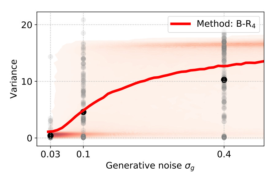 Figure 1
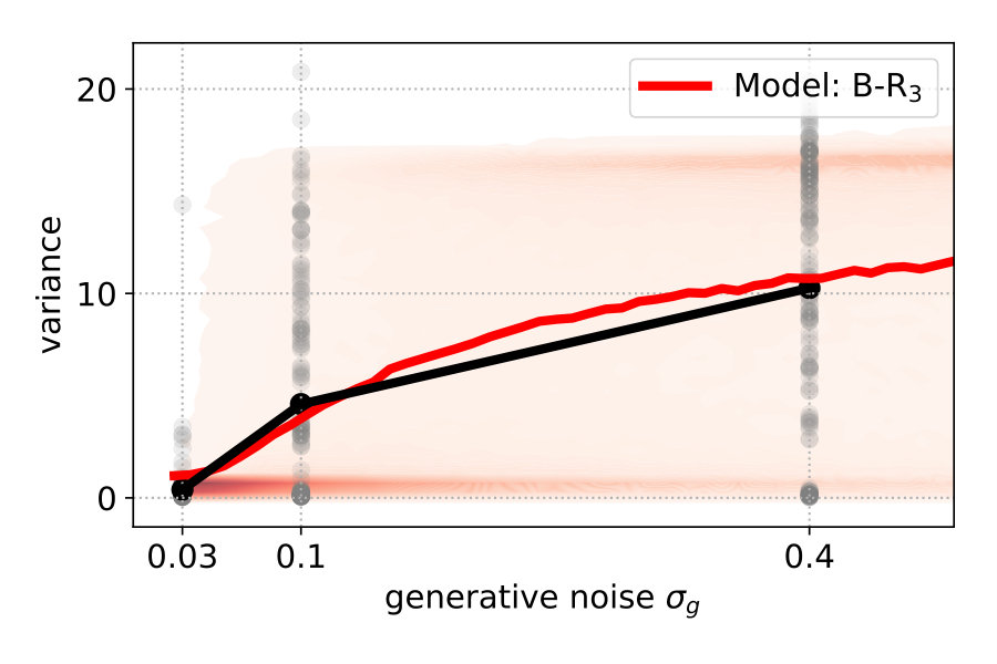 Figure 2
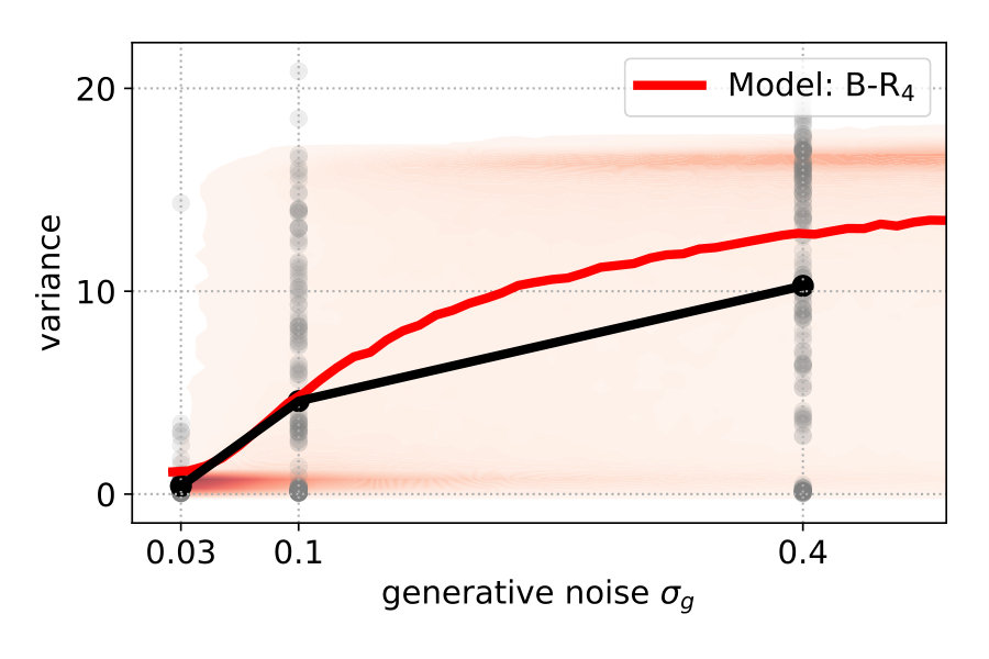 Figure 3
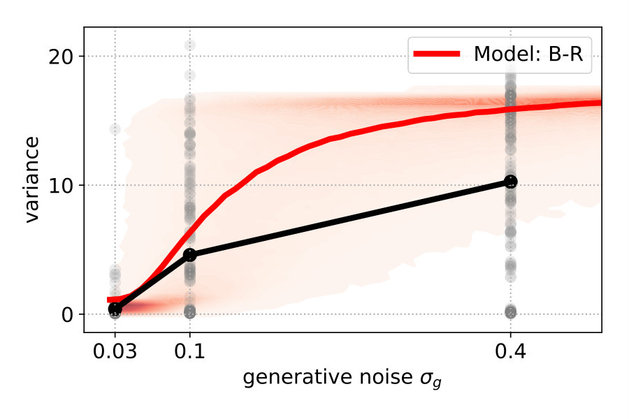 Figure 4
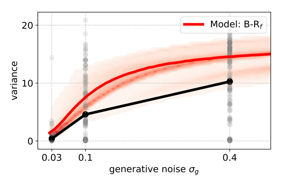 Figure 5
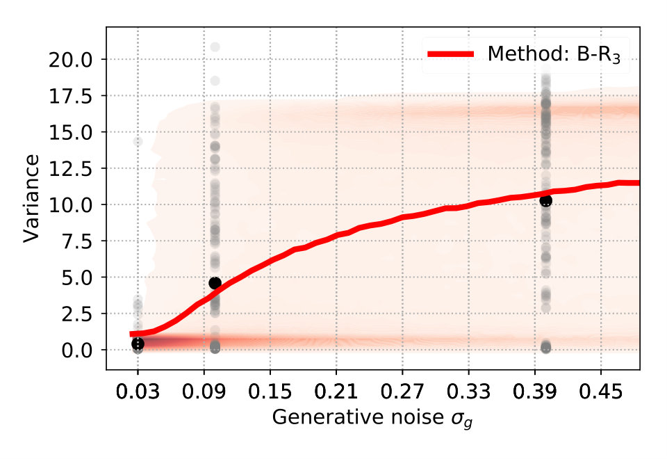 Figure 6
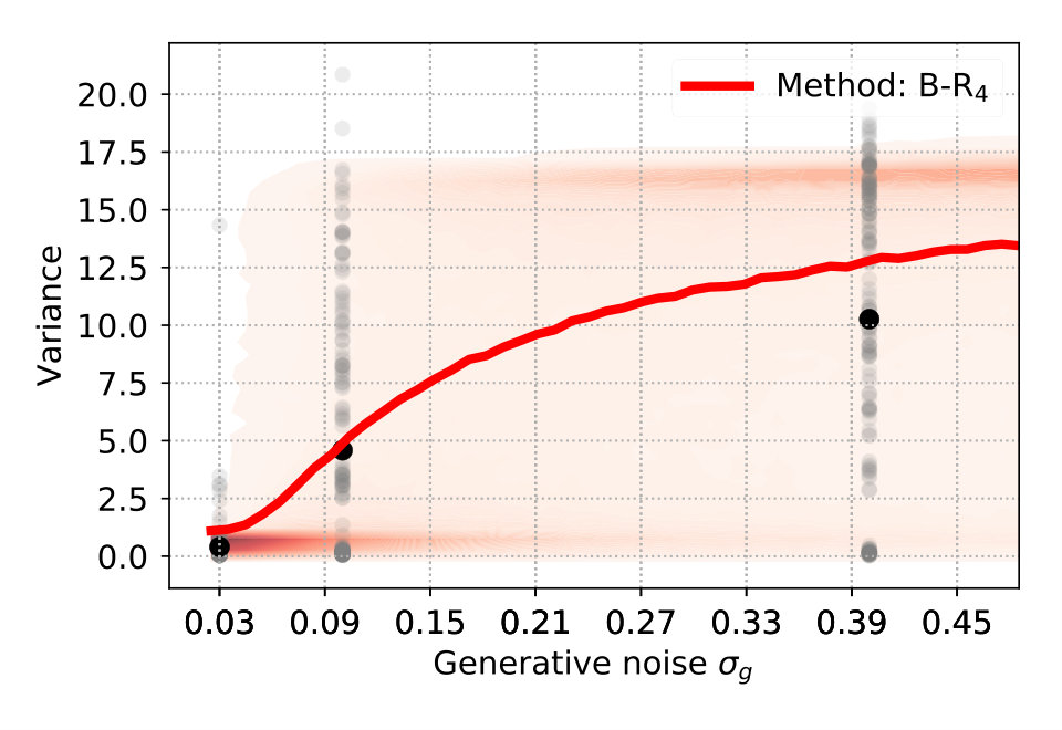 Figure 7
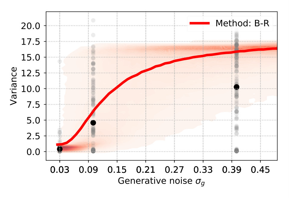 Figure 8
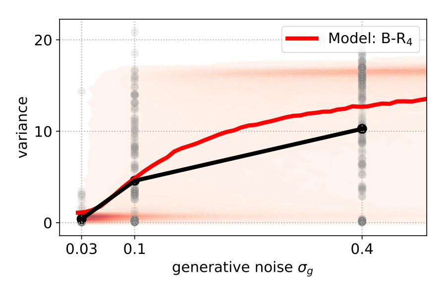 Figure 9
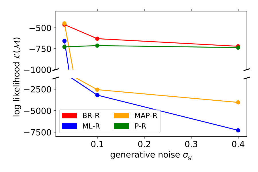 Figure 10
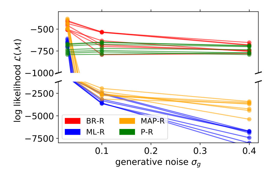 Figure 11
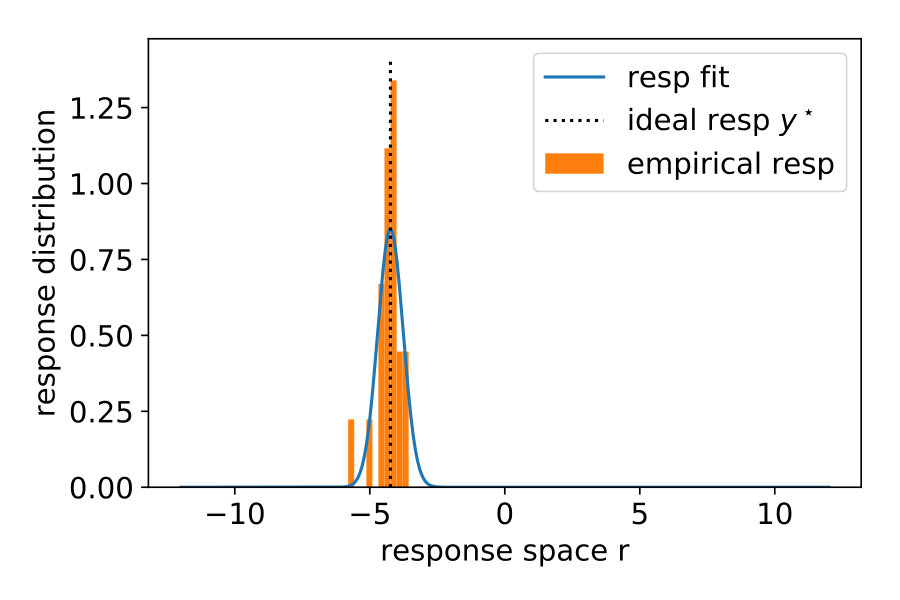 Figure 12
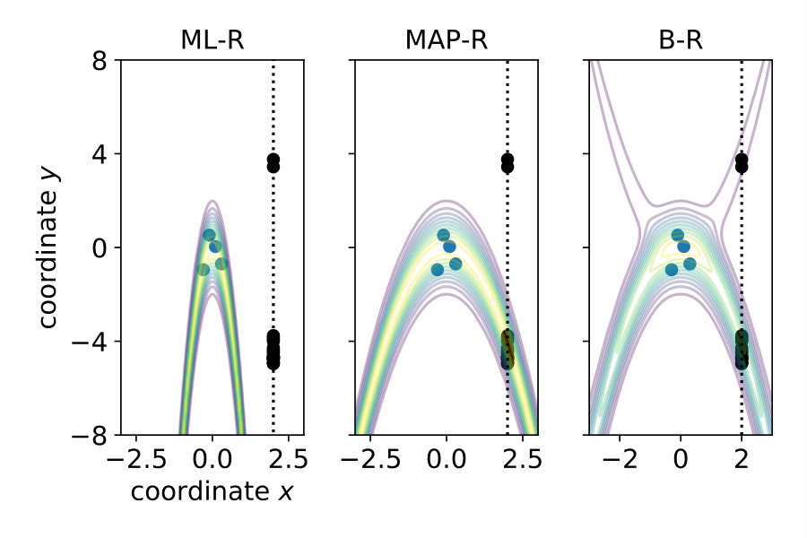 Figure 13
 Figure 14
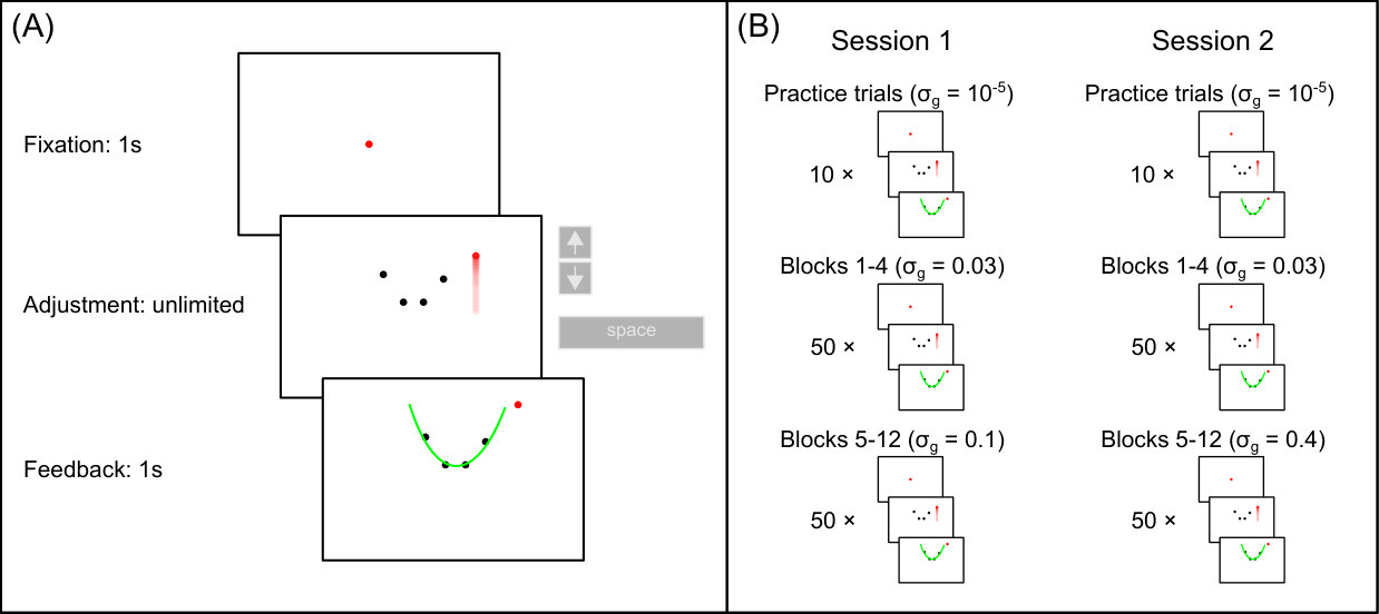 Figure 15
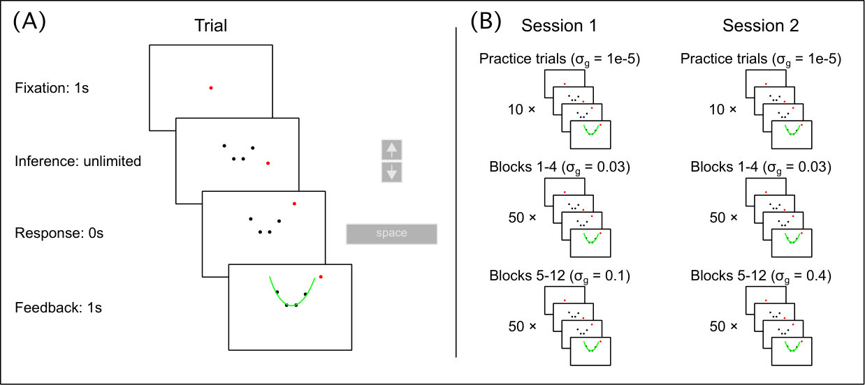 Figure 16
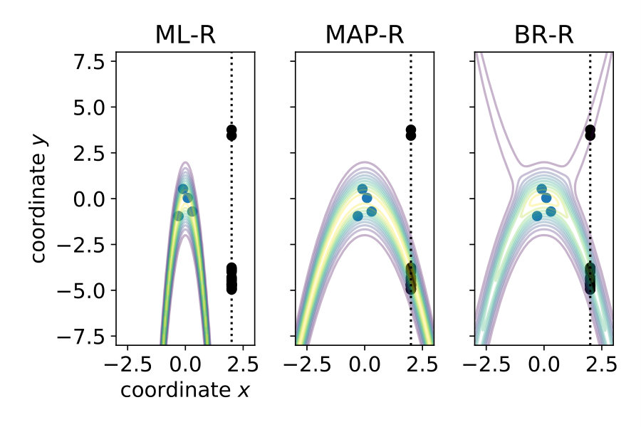 Figure 17
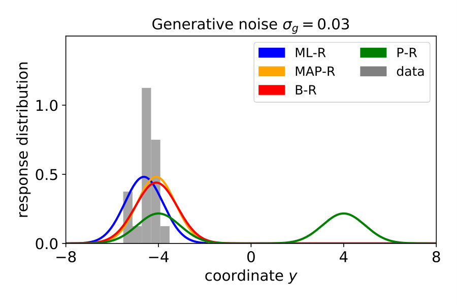 Figure 18
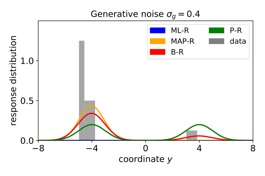 Figure 19
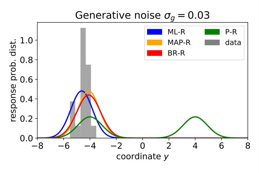 Figure 20
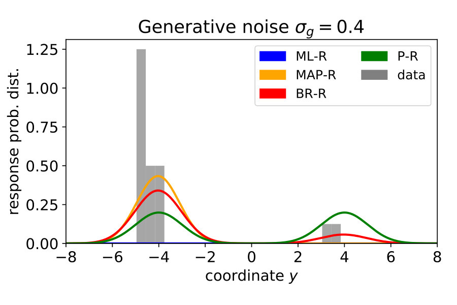 Figure 21
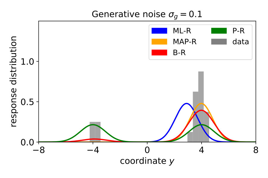 Figure 22
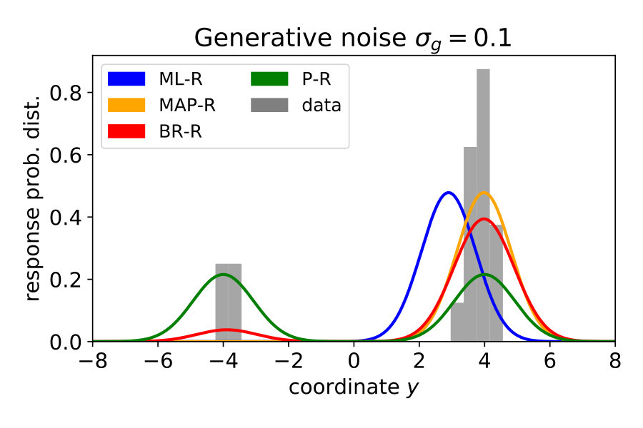 Figure 23
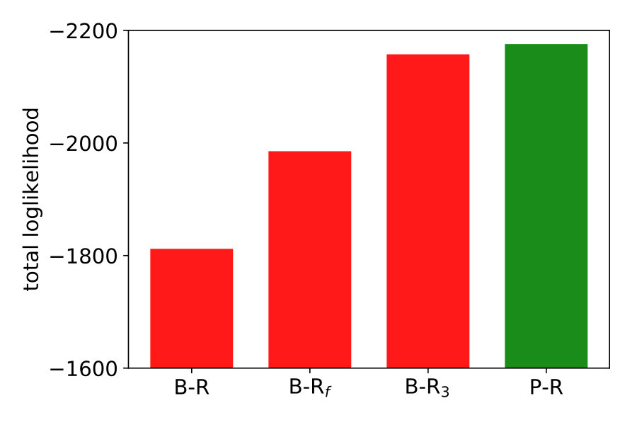 Figure 24
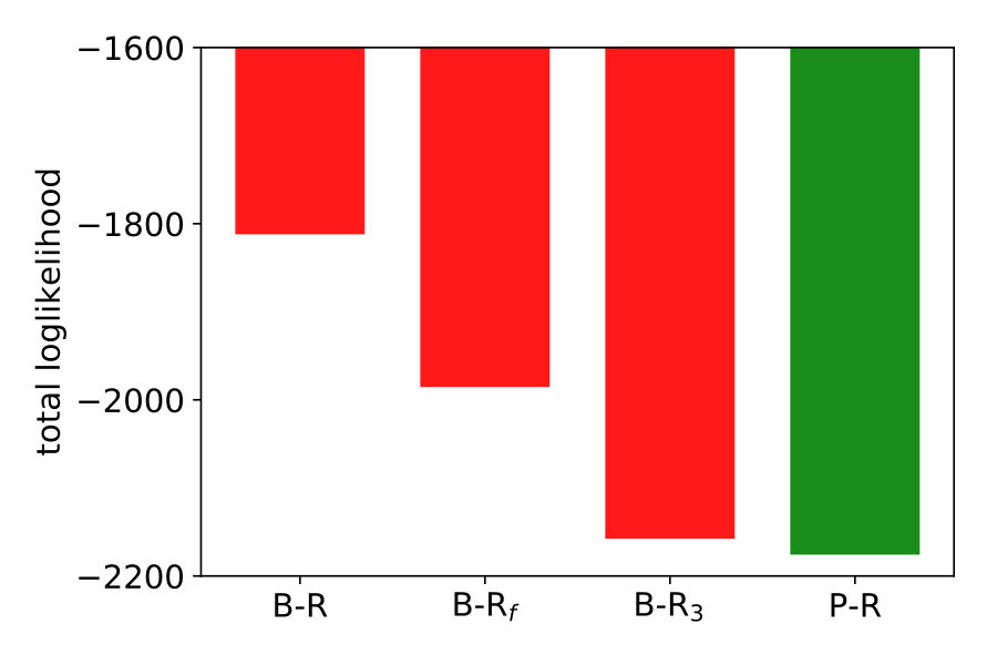 Figure 25
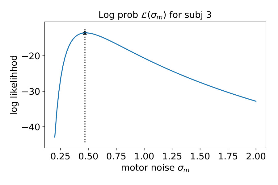 Figure 26
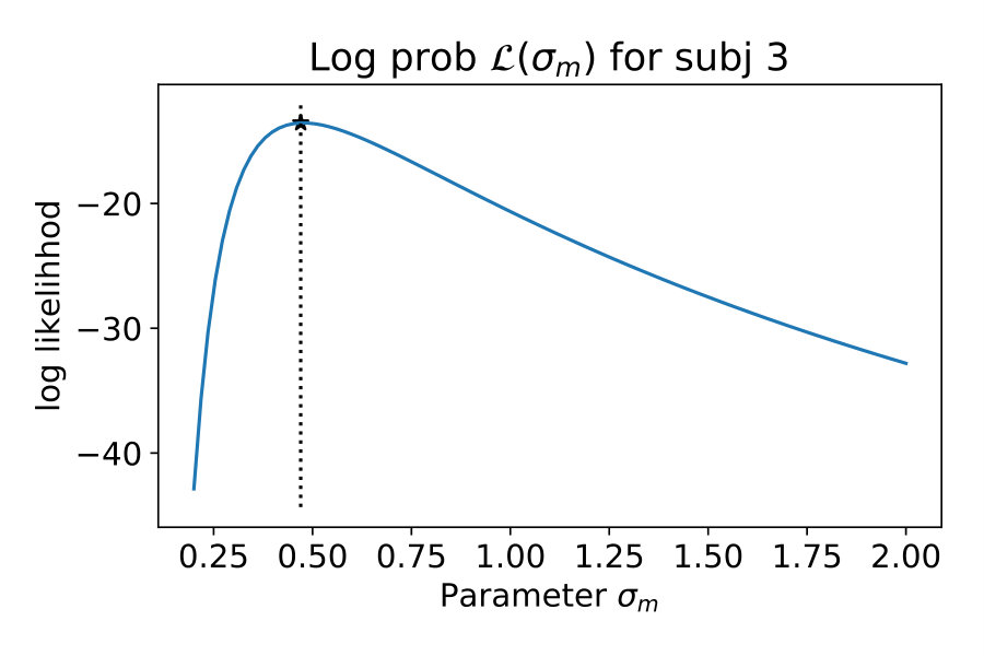 Figure 27
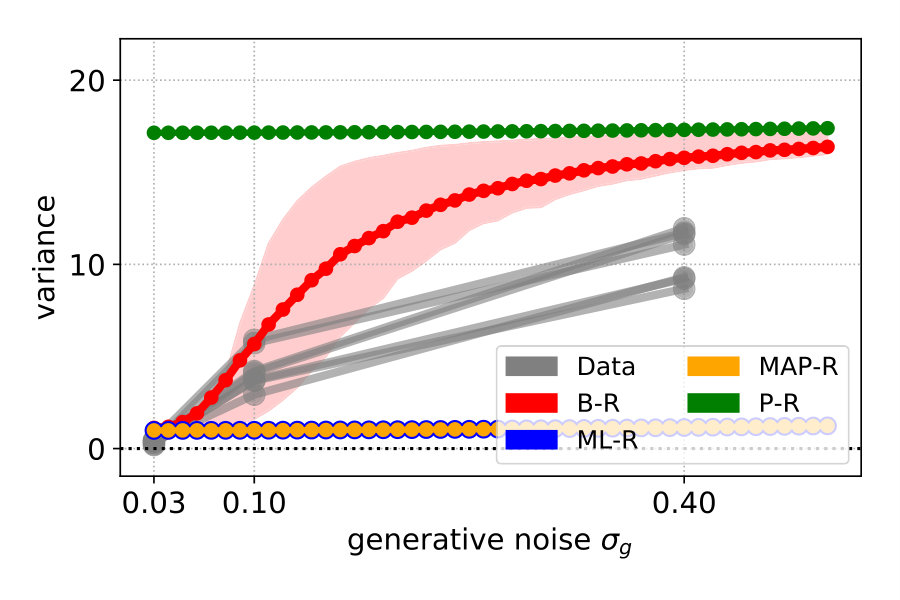 Figure 29
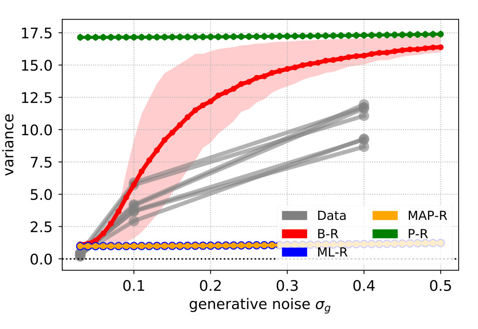 Figure 30
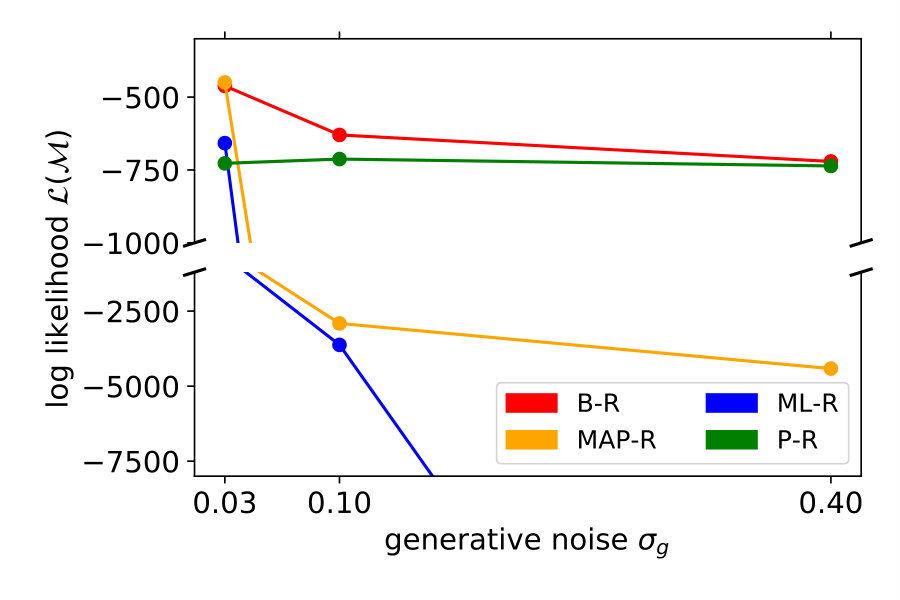 Figure 31
 Figure 32
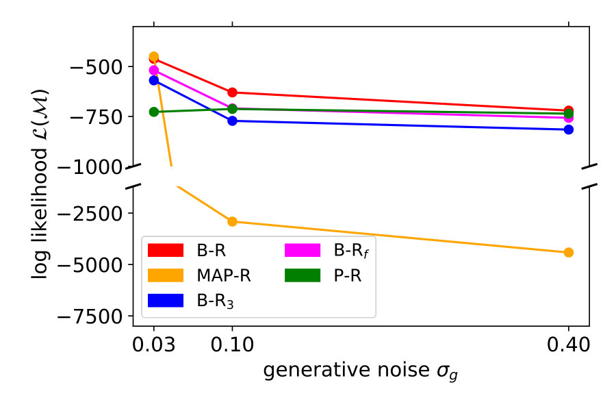 Figure 33
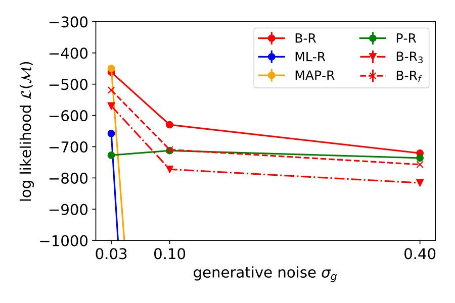 Figure 34
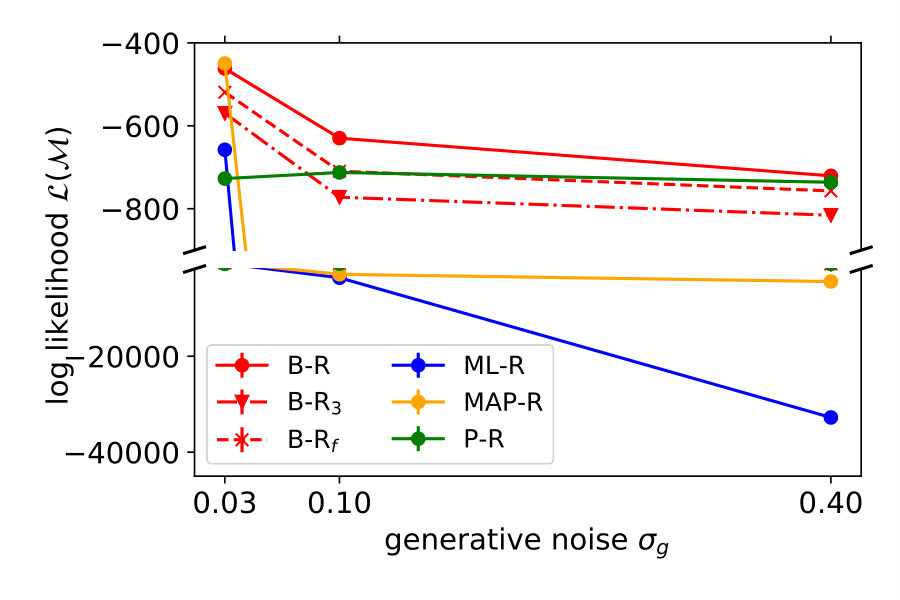 Figure 35
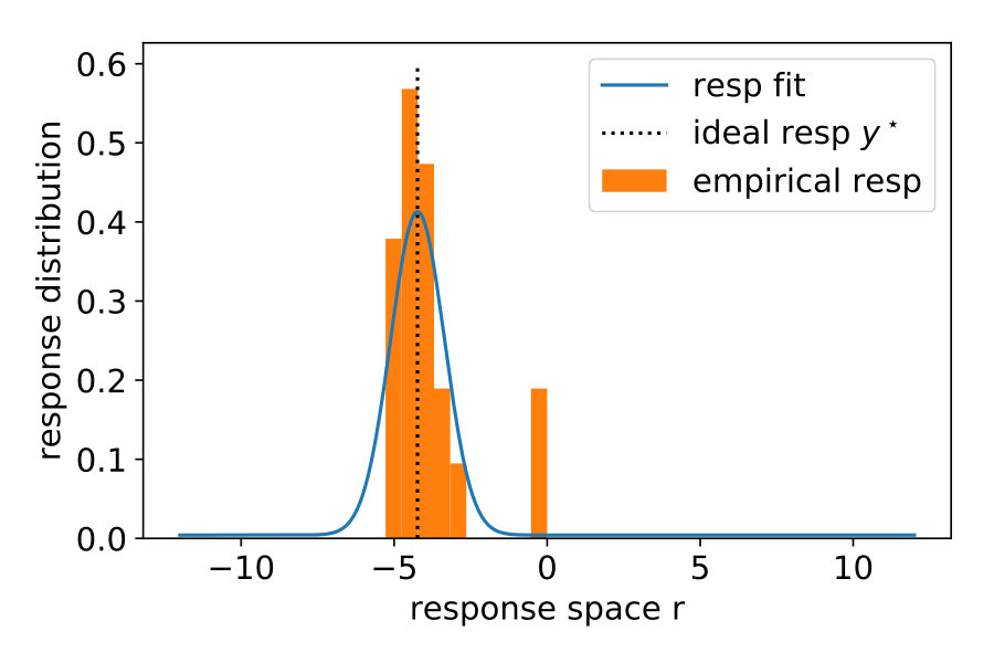 Figure 36
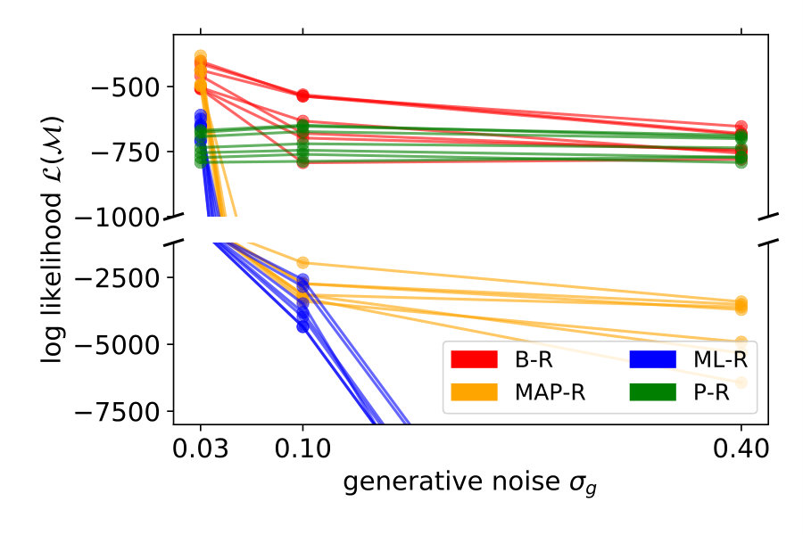 Figure 37
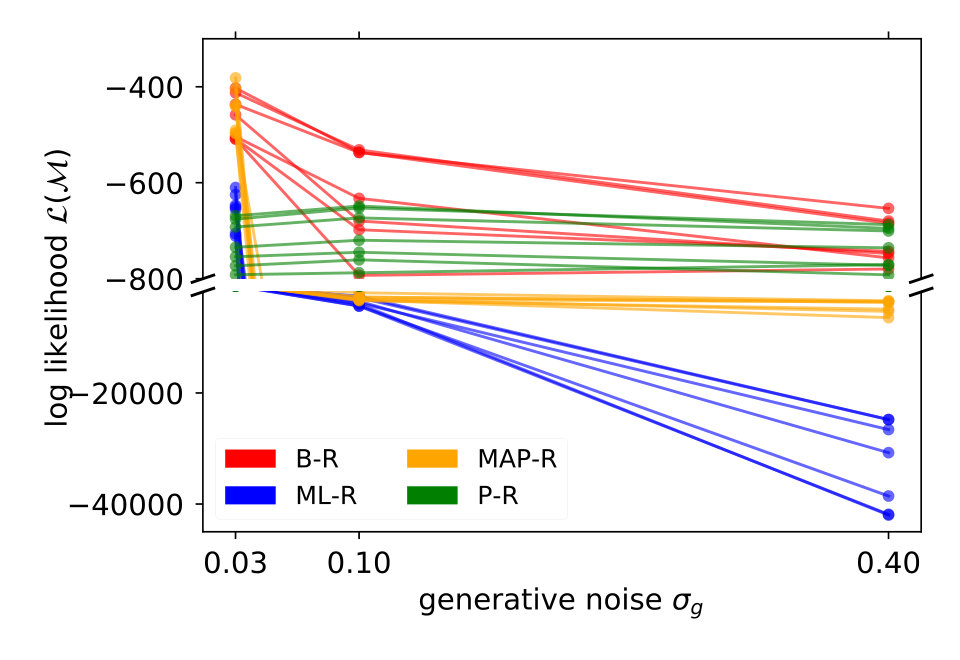 Figure 38
Peer Reviews
No public reviews on file for this paper yet. If you reviewed it on a platform where reviews are public (OpenReview, ICLR, NeurIPS, ICML), you can paste yours below so the community can read it here.
Videos
No videos yet. Explain this paper in a talk, walkthrough, or lecture? Add one.
\templatetype
pnasresearcharticle
\leadauthorJegminat \significancestatementA central function of the brain is learning a model of the world from sensory inputs. Taking into account the noise and ambiguity of these inputs, the brain works with levels of belief rather than single values. Previous research mostly focused on how the brain represents its beliefs about the outside world. Here, we ask the following question: how do different levels of belief influence predictions made by the brain’s model? We consider three methods of doing this, ranging from "not at all" to "totally", and compare them to human performance in a visual experiment. Our results suggest that brains are well aware of their degree of belief when making predictions. \authorcontributionsJ.J., M.J., M.P. M.H. and J.P. designed research; M.J., M.P., M.H. conducted the experiment; J.J., J.P. analyzed data; and J.J., M.J., M.H., J.P. wrote the paper.
\authordeclarationThe authors declare no conflict of interest here. \correspondingauthor2To whom correspondence should be addressed. E-mail: [email protected]
Bayesian regression explains how human participants handle parameter uncertainty
Jannes Jegminat
Department of Physiology, University of Bern, 3012 Bern, Switzerland
Institute of Neuroinformatics and Neuroscience Center Zurich, ETH and the University of Zurich, 8057 Zurich, Switzerland
Maya A. Jastrzębowska
Laboratory of Psychophysics (LPSY), Brain Mind Institute, School of Life Sciences, École Polytechnique Fédérale de Lausanne (EPFL), 1015 Lausanne, Switzerland
Laboratory for Research in Neuroimaging (LREN), Department of Clinical Neuroscience, Lausanne University Hospital and University of Lausanne, 1011 Lausanne, Switzerland
Matthew V. Pachai
Laboratory of Psychophysics (LPSY), Brain Mind Institute, School of Life Sciences, École Polytechnique Fédérale de Lausanne (EPFL), 1015 Lausanne, Switzerland
Department of Psychology, York University, ON M3J 1P3 North York, Canada
Michael H. Herzog
Laboratory of Psychophysics (LPSY), Brain Mind Institute, School of Life Sciences, École Polytechnique Fédérale de Lausanne (EPFL), 1015 Lausanne, Switzerland
Jean-Pascal Pfister
Department of Physiology, University of Bern, 3012 Bern, Switzerland
Institute of Neuroinformatics and Neuroscience Center Zurich, ETH and the University of Zurich, 8057 Zurich, Switzerland
Abstract
The human brain copes with sensory uncertainty in accordance with Bayes’ rule. However, it is unknown how the brain makes predictions in the presence of parameter uncertainty. Here, we tested whether and how humans take parameter uncertainty into account in a regression task. Participants extrapolated a parabola from a limited number of noisy points, shown on a computer screen. The quadratic parameter was drawn from a prior distribution, unknown to the observers. We tested whether human observers take full advantage of the given information, including the likelihood function of the observed points and the prior distribution of the quadratic parameter. We compared human performance with Bayesian regression, which is the (Bayes) optimal solution to this problem, and three sub-optimal models, namely maximum likelihood regression, prior regression and maximum a posteriori regression, which are simpler to compute. Our results clearly show that humans use Bayesian regression. We further investigated several variants of Bayesian regression models depending on how the generative noise is treated and found that participants act in line with the more sophisticated version.
keywords:
Bayesian regression Psychophysics Parameter uncertainty
doi:
www.pnas.org/cgi/doi/10.1073/pnas.XXXXXXXXXX
\dates
This manuscript was compiled on
\dropcap
The brain evolved in an environment that requires fast decisions to be made based on noisy, ambiguous and sparse sensory information, noisy information processing and noisy effectors. Hence, decisions are typically made under substantial uncertainty. The Bayesian brain hypothesis states that the brain uses the framework of Bayesian probabilistic computation to make optimal decisions in the presence of uncertainty (1, 2, 3). A large body of research has established that many aspects of cognition are indeed well described by Bayesian statistics. These include magnitude estimation (4), color discrimination (5), cue combination (6), cross-modal integration (7, 8), integration of prior knowledge (9, 10) and motor control (11, 12, 13).
Most of these experimental studies can be cast into the problem of estimating a hidden quantity from sensory input. Much fewer experimental studies have been performed on regression tasks (but see (14) for an overview, and, e.g., (15, 16, 17)). In a regression task, the aim is to learn the mapping from a stimulus to an output after having been exposed to a training data set of associations between stimulus and its corresponding . Since the mapping from to can be probabilistic, the aim of regression is to find an expression for . Classification tasks (such as object recognition) or self-supervised tasks such as estimating the future position of an object from past observations are just a few examples from a long list of regression tasks performed on a daily basis.
The machine learning literature contains many solutions to the regression problem, such as nonlinear regression, support vector machines, Gaussian processes or deep neural networks (see (18) for an introduction). It is unclear, however, how humans perform regression tasks. Most of the machine learning solutions rely on the assumption that the mapping from to is parametrized by a set of parameters , such that the original regression problem of finding is replaced by a parameter estimation problem, i.e., finding the best set of parameters for the parametrized mapping . However, this approach is not Bayesian since no uncertainty over the parameters is included in the regression model.
The Bayesian approach to regression proceeds in two steps (19). First, the posterior distribution over the parameters is computed from the observed data . Then, this posterior is used to compute the posterior predictive distribution by integrating over the parameters:
[TABLE]
Taking into account the uncertainty over parameters is particularly relevant for predictions when the data set size is small compared to the number of parameters. Indeed, taking into account the uncertainty helps to generalize to unknown data and thereby alleviates overfitting. Parameter uncertainty also plays a key role in computing the prediction uncertainty. Both of these aspects – overfitting on small data sets and lack of prediction uncertainty – currently limit the power of deep neural network models (20, 21). These models have millions of parameters and their performance grows with the number of layers (22, 23). To prevent overfitting, training these models requires ever larger and more expensive training sets.
It is interesting to note that classic DNNs do not use weight uncertainty and are therefore limited in their ability to compute the prediction uncertainty. Recently, the idea of computing the probability distribution over weights in DNNs and using it for prediction has gained traction and given rise to the so-called Bayesian Neuronal Network (BNN), for example (24, 25). BNNs promise better performance in the low-data regime. Additionally, BNNs output their prediction uncertainty, which is crucial when the cost of decisions is unequally distributed as is usually the case in behavioural tasks (26, 27, 28).
Here we ask if humans take advantage of Bayesian regression. To address this question, we conducted the following psychophysical experiment. Participants sat in front of a screen on which 4 points from a noisy parabola were shown. Their task was to correctly extrapolate the parabola, i.e., to find the vertical position of the parabola at a given horizontal location. The quadratic parameters of the parabolas were drawn from a bimodal prior distribution, designed to make the parabolas face either upwards or downwards. After recording the participant’s response, we showed the parabola that generated the dots as feedback. This feedback enabled the participants to learn both the prior and the generative model. Because we wanted to test to what extent participants made decisions in accordance with a Bayesian regression strategy, we varied the level of noise of the parabola. The rationale is that the higher the noise level, the higher the uncertainty about the correct parameter and, according to Bayesian regression, the more participants should rely on the prior. We found that Bayesian regression indeed explained participants’ responses better than maximum likelihood regression and maximum a posteriori regression. The latter two models are widely used by applied statisticians (29, 30, 31, 32, 33, 34, 35, 36, 37) and also in psychophysical modelling (38) but fail to account for parameter uncertainty.
1 Results
1.1 A novel paradigm to test regression
In each trial, we chose the parameter of a parabola from a fixed prior distribution . Participants were shown 4 dots which were on this parabola, but the parabola itself was not shown. We had 20 such 4-dot stimuli, which we repeated 20 times each. For a certain 4-dot stimulus , the parameter was always the same. The x-positions of the 4 stimulus dots were fixed across all trials and were rather close to the vertex of the parabola. The parameter was either positive (parabola opening upwards) or negative (parabola opening downwards), with the same probability, i.e., 0.5. The prior distribution was bimodal with means of and standard deviations of 0.1 (see Material and Methods section 2.1). We did not tell observers about the prior probability distribution. Also unbeknown to the observers, we jittered the dots for each stimulus along the y-axis by adding zero-mean Gaussian noise of a certain level . The jitter was the same for all 20 repetitions of a stimulus . A fifth dot was presented to the right of the 4-dot stimulus, always at the same x-position . Participants could move the fifth dot up and down along the y-axis by using the up and down arrow keys. Participants were asked to adjust the y-position so that the dot correctly extrapolated the parabola. After the adjustment, we showed the generating parabola and the adjusted point as feedback.
Because we wanted to test to what extent observers rely on prior information, we used low, middle and high values of . The rationale is that the higher the noise level, the higher the uncertainty (the lower the likelihood) and the more participants rely on the prior. Thus, for each participant and each of the 3 noise levels, we ran 20 4-dot stimuli with 20 repetitions, which were randomly ordered (Figure 1, right). The set of responses to a 4-dot stimulus is . The different regression models make different predictions as to the extent to which participants use the generative probability and the prior .
1.2 The regression models
We considered four regression models. Maximum likelihood regression (ML-R) does not take the prior distribution into account and computes only the point estimate of that maximizes the likelihood . The maximum a posteriori model (MAP-R) combines the likelihood with the prior distribution to compute the mode of the posterior distribution . The Bayesian regression (B-R) model takes the entire posterior distribution into account:
[TABLE]
Note that in the previous three models, we assumed that participants know the generative noise () – an assumption that will be relaxed in Section 1.4. As a null model, we included prior regression (P-R), which replaces the posterior with the prior, i.e., it does not use the likelihood. For more details, see Materials and Methods Section 2.2. To model participants’ responses, we also included the internal sources of noise arising during neural processing, decision making and the execution of motor action. To this end, we presented the same noise-free () stimulus 20 times and measured the variability of the responses . We then transformed the predictive distribution into a (predicted) response distribution over by convolving with a Gaussian (see Materials and Methods Section 2.3). Figure 2 shows the responses of a typical subject along with the model predictions. Both ML-R and MAP-R ignore one of the modes (here, the mode corresponding to a parabola which opens upwards). In addition, the parabola predicted by ML-R is much thinner (i.e., the absolute value of the quadratic parameter is high) than the parabola that the participant responded with because ML-R ignores the prior but humans likely do not. In the low noise regime () (Figure 2 (B)), the participant’s unimodal response distribution rules out the null model, which shows a second mode. In the high noise regime () (Figure 2 (D)), MAP-R and ML-R fail to account for the fact that the participant distributed his responses across both modes. In the intermediate noise regime () (Figure 2 (C)), the participant sometimes gave tightly clustered responses and sometimes distributed them across both modes. Generally, B-R captures the participant’s responses best as compared to the other models.
1.3 B-R outperforms the other models
We showed the performance of a typical participant in Figure 2. Now, we compare model performance across all seven participants. For each of the seven participants individually, we computed the log probability that the model reproduces their responses, i.e., the y-position adjusted by the participant. We summed these log probabilities for all of the 20 stimuli as a measure of the quality of the model. Figure 3 shows these values for each noise level and participant separately (left) and averaged across participants (right). The higher the value, the better the model performance.
For all noise levels, B-R is among the highest performing models. At the lowest and highest noise level, MAP-R and P-R show similar performance to B-R, respectively. The results are consistent across participants. At low noise levels, MAP-R and B-R perform equally well because the stimulus is unambiguous. In this case, the posterior belief about the quadratic parameter is well approximated by a single value, the MAP. In contrast, at high noise, the prior is more important in determining the posterior belief about the quadratic parameter. In fact, the posterior closely approximates the bimodal prior. For this reason, B-R and P-R perform similarly well. At the medium noise level, the posterior belief is influenced by the prior and likelihood to approximately the same degree. In this case, B-R outperforms the other models because it takes full advantage of the posterior distribution, in particular, its bimodality. At medium and high noise levels, even P-R clearly outperforms MAP-R and ML-R because the latter two models predict unimodal responses, i.e., they predict that the parabola either opens up- or downwards depending on the stimulus . Their failure to model responses belonging to the other mode is strongly punished by the log-likelihood measure because the model predicts a close-to-zero probability for these responses.
1.4 B-R explains the generative noise-dependent increase in response variance
When participants responded with a position that was far from a mode of the predicted response distribution, the log-likelihood strongly punished the corresponding model. To complement the log-likelihood analysis with a metric that is more sensitive to the overall response distribution, we used the variance. For each stimulus , we computed the variance of the 20 recorded responses. For example, if all responses are located in the upper mode, the variance is close to zero. If they are distributed evenly across both modes, the variance is close to 16, which corresponds to the variance of the prior P-R. To obtain a single value for each participant and each noise level , we averaged the variance values across stimuli . This value represents the averaged variance of responses at stimuli generated at . Next, we compared the average variance with the predicted averaged variance of each model. To this end, we generated a large number of stimuli from and averaged the variance of the predicted response distributions (see Materials and Methods Section 2.4).
Figure 4 (top left) compares the averaged variance of the participants’ responses (gray) with the model predictions (color-coded). The B-R variance changes strongly with the noise level. The reason is that the generative noise determines the contribution of likelihood and prior for the responses; thus, the predicted responses change from a unimodal to bimodal in B-R. As a result, the B-R (red) variance values smoothly transition from the MAP/ML variances at the low noise level () to the P-R variance at the high noise level (). This is not the case in the other models.
There is some discrepancy between the data from the participants and the prediction of B-R. At high noise (), the participants’ variance increases more slowly than what B-R predicts. This means that participants cluster their responses close to one of the modes more often than predicted.
To explain the discrepancy, we tested two additional variants of B-R. Full Bayesian regression B-Rf and three-point Bayesian regression B-R3. Both are based on the idea that participants do not regard the generative noise as constant but rather infer (in B-Rf) or estimate (in B-R3) it on a per-trial basis. When participants assumed that the generative noise was smaller than the one we used to generate the points, their responses were more clustered. As a consequence, the average variance decreased. This happened when the four stimulus points were by chance aligned on a parabola. When we computed the averaged variance with classical B-R, we used the true generative noise which was, in this case, larger than the estimated noise. Since the noise determines how much participants rely on the prior and likelihood relative to each other, the averaged variance of the prediction was larger than in the data.
Both additional variants of B-R consider the noise on a trial-by-trial basis, but they differ in how they do it. While B-R only infers the quadratic parameter , B-Rf extends the inference to the noise level as well. Since the generative model does not specify a prior over the (fixed) hyperparameter noise , we used an exponential prior and set its mean to the fixed hyperparameter (see Material and Methods eq. 9). B-Rf uses the joint posterior over and to predict further responses. When the 4-dot stimulus closely resembled a parabola, the posterior belief over was highly peaked around a value that was smaller than the actual generative noise parameter. Thus, we expected more clustered responses and predicted a lower averaged variance.
B-R3 differs from B-R in that it includes the preprocessing step of estimating the generative noise on a trial-by-trial basis and treating the left or rightmost stimulus point as an outlier. The noise estimate is then used in standard B-R. The easiest approach to achieve this is using the maximum-likelihood estimator of the noise and all four stimulus points. Often, the maximum likelihood estimate was smaller than the fixed hyperparameter, reducing the averaged variance (see Supplementary Information). Data and prediction matched almost perfectly if we allowed for the possibility to disregard outliers during the estimation (see Materials and Methods section 2.2).
Figure 4 (top right and bottom) show the variance distribution predicted (red, mean: line) by B-R, B-Rf and B-R3. The data (gray, mean: black) is pooled across participants. In the data, there is a portion of almost zero-variance responses for all noise levels. The fraction of these highly clustered responses decreases as the generative noise increases but remains present for all experimental conditions. Only B-R3 captures this aspect of the data. Besides this, the variances associated with both variants of B-R rise more slowly than that of the original B-R, supporting the idea that the generative noise is indeed jointly estimated with the quadratic parameter. The comparison between measured and predicted responses strongly favours B-R. B-R with as a fixed hyperparameter overestimates the increase in variance compared to the data. By using two variants of B-R, we show that this discrepancy can be explained by assuming that participants estimate the generative noise on a per-trial basis. The two additional variants of B-R perform slightly worse than the original B-R in terms of the log-likelihood but still better than all other models (see Supplementary Information).
In summary, both the likelihood-based model comparison and the response variance results strongly favour B-R.
2 Discussion
Participants adjusted a dot such that it fits on a parabola determined by four other dots. We used the variance and the log-likelihood to compare the participants’ responses to the predictions of four regression models: ML-R, MAP-R, P-R and B-R. Out of these, B-R best explained the participants’ responses across different levels of stimulus noise. In particular, B-R interpolated between the variances of MAP-R at low noise levels and P-R at high noise levels. We found the same trend in the data, although B-R predicted larger values for the variance at high noise levels. We could explain this discrepancy with the assumption that participants estimate the noise level per trial and then apply it. We conclude that in our task, participants are capable of implicitly performing or at least approximating a complicated integral over the posterior distribution of the parameter given the data.
The rationale behind our experimental design was to use the simplest possible setup to study if humans perform Bayesian regression. Our one-dimensional response space was easy to visualize and the amount of data needed to compare the predictive and empirical distributions was limited. Bayesian regression easily extends beyond the simple low dimension problem of a single quadric nonlinearity to problems with higher dimensional parameters, such as polynomials of arbitrary degree, and to other basis functions, such as Gaussians. Future research needs to study to what level of complexity humans perform Bayesian regression. There is some evidence that the brain uses sampling to represent high dimensional distributions (39). This representation of distributions scales to high dimensions and offers a potential way of evaluating the high dimensional integral needed for Bayesian regression.
In our analysis, we assumed that participants know the generative model, including the prior over the parameters. Without this assumption, we would have had to account for potential temporal dynamics of learning with a participant-specific, time-dependent prior. For instance, it might take participants a non-negligible amount of time to learn the generative model or their responses could be influenced by immediately preceding trials. To avoid such complications, we showed the generative parabola after each trial.
Our work was inspired by the growing emphasis on parameter uncertainty in the machine learning community; however, it is important to highlight that function learning and extrapolation have been studied before. The function learning literature has addressed which types of functions humans can learn (40), how batch or sequential data representation affects learning (17), to what extent human behaviour can be modelled by parametric functions (41) and how well humans extrapolate (16). However, to the best our knowledge, these studies have so far failed to conduct a minimal experiment to establish that humans behave in accordance with Bayesian regression. Our contribution will help to better understand the brain’s remarkable ability to learn and generalise from very little data and underpins the power of Bayesian regression as a framework in psychophysical modelling.
\matmethods
2.1 Stimulus generation from the bimodal prior
Here, we describe in detail how stimuli are generated. On the jth trial, participants are presented with a stimulus consisting of points in a 2-dimensional space: . For each stimulus, we fix the x-values and generate the y-coordinates from a Gaussian generative model with a parabolic non-linearity and the generative parameter, :
[TABLE]
The parameter is drawn from a mixed Gaussian prior
[TABLE]
where the parameter set consists of the mean , the standard deviation and the mixing coefficient . We denote the total set of hyperparameters (suppressed for notational clarity), from the prior and the generative probability, by . Each parameter corresponds to a generative parabola. Given this model and given a stimulus , we asked participants to predict the y-component at , which is equivalent to mentally fitting a parabola to the four stimulus points and estimating the point of intersection with a vertical line at .
To train participants on the generative model and the prior, we showed participants the generative parabola after each trial. In total, we showed a set of 20 unique stimuli for each of the three noise levels , and each unique stimulus was repeated 20 times. We denote the set of the 20 responses to the jth stimulus as . This amounts to a total of 400 trials per noise level. The order of the stimuli was randomized. Figure 1 shows the set-up.
2.2 Regression models
In each trial, the participants carried out an inference step and a prediction step. During the inference step, they inferred information about the quadratic parameter based on the presented data (i.e., stimulus) . The information they inferred depends on the inference model participants use. The inferred information was then used for a subsequent prediction . Therefore, the participants overall task was to compute the predictive distribution: .
Prior regression (P-R) is our null model. P-R assumes that participants make predictions based on their prior belief but disregard information from the stimulus:
[TABLE]
Maximum likelihood regression (ML-R) relies only on the likelihood maximizing parameter, :
[TABLE]
Maximum a posteriori regression (MAP-R) uses the parameter that maximizes the posterior :
[TABLE]
Bayesian regression (B-R) uses the entire posterior for making predictions by marginalizing over it:
[TABLE]
Full Bayesian regression (B-Rf) loosens the assumption that participants treat as a hyperparameter. Including with an exponential prior in Bayesian regression generalizes eq. 8:
[TABLE]
We chose an exponential prior because it has only one free parameter. By setting the expectation over equal to the actual hyperparameter , we eliminated this degree of freedom and retained our fitting free approach (see Supplementary Information).
Three point regression (B-R3) assumes that participants use an estimate based on points. The posterior predictive is computed exactly as in ordinary B-R (eq. 8) except for the following replacement where is computed in a two step procedure. First, we obtained two maximum likelihood estimates of the generative noise by ignoring the left most and the right most point. Second, the minimum of these two was . We also tested as an alternative but concluded that gave a more convincing account of the observed variance (see Supplementary Information Figure S1).
2.3 Participants’ internal noise
To predict the participants’ responses from the regression models’ output , we had to account for the internal noise of the participants. We did this by showing a noise-free parabola and fitting a Gaussian with variance to each participant’s response variability: . As explained in more detail in the Supplementary Information, the predicted response distribution is then
[TABLE]
2.4 Model comparison
We used the log-likelihood and the variance to compare the predicted and empirical response distributions.
Log likelihood. To compute the log likelihood for a model across all response at a given noise level , we summed the individual log likelihoods of each response (the log of eq. 10) across all stimuli :
[TABLE]
Variance prediction
As a independent comparison of the data and the predicted response distribution, we used the variance. For each of the 20 stimuli we obtained a single empirical value from the 20 responses recorded. Hence, at each noise level , we have a variance distribution:
[TABLE]
where high variance values reflect ambiguous and difficult stimuli while low values indicate easy stimuli, prompting participants to give very similar responses across trials. The predicted variance distribution is expressed by
[TABLE]
where we used 1000 stimulus samples and computed the variance analytically (see Supplementary Information). We use this distribution to compute the means and quantiles shown in fig. 4 (top left) and the color-coded density in the other plots.
2.5 Participants
Seven participants (3 females, 4 males, ages 21-27) participated in the experiment. The experiment was programmed using custom software implemented in MATLAB. Stimuli were presented on a 1920x1080 (36 pixels/cm) monitor with a refresh rate of 120 Hz. Participants viewed the display binocularly. Each trial comprised a fixation dot presented for 1 s followed immediately by presentation of the stimulus (with 5 arcmin point diameter). Participants moved a red point up or down using the up and down arrow keys to indicate the vertical position of the parabola at the given horizontal location. See Supplementary Information for more details.
\showmatmethods
\acknow
We would like to thank Frank Jäkel for his insightful input. J.J. and J.-P.P. were supported by the Swiss National Science Foundation grants PP00P3_150637 and 31003A_175644. M.A.J., M.P. and M.H.H. were supported by the SNF grant ’Basics of visual processing: from elements to figures’ (176153).
\showacknow
The reference list from the paper itself. Each links out to its DOI / PubMed record.
- 1(1) Knill DC, Pouget A (2004) The bayesian brain: the role of uncertainty in neural coding and computation. TRENDS in Neurosciences 27(12):712–719.
- 2(2) Vilares I, Kording K (2011) Bayesian models: the structure of the world, uncertainty, behavior, and the brain. Annals of the New York Academy of Sciences 1224(1):22–39.
- 3(3) Friston K (2012) The history of the future of the bayesian brain. Neuro Image 62(2):1230–1233.
- 4(4) Petzschner FH, Glasauer S (2011) Iterative bayesian estimation as an explanation for range and regression effects: a study on human path integration. Journal of Neuroscience 31(47):17220–17229.
- 5(5) Olkkonen M, Mc Carthy PF, Allred SR (2014) The central tendency bias in color perception: Effects of internal and external noise. Journal of Vision 14(11):1–15.
- 6(6) Ernst MO, Banks MS (2002) Humans integrate visual and haptic information in a statistically optimal fashion. Nature 415(6870):429.
- 7(7) Alais D, Burr D (2004) Ventriloquist Effect Results from Near-Optimal Bimodal Integration. Current Biology 14(3):257–262.
- 8(8) Shams L, Kim R (2010) Crossmodal influences on visual perception. Physics of Life Reviews 7(3):269–284.