Critical behavior at the localization transition on random regular graphs
K. S. Tikhonov, A. D. Mirlin

TL;DR
This paper investigates the critical behavior of the Anderson localization transition on random regular graphs, accurately determining the critical disorder and analyzing the correlation length divergence with notable corrections to scaling.
Contribution
It provides the first precise estimate of the critical disorder and characterizes the critical divergence of the correlation length on random regular graphs.
Findings
Critical disorder W_c = 18.17 ± 0.01 was determined.
Correlation length diverges as (W_c - W)^(-1/2) near the transition.
Pronounced corrections to scaling similar to high-dimensional and many-body localization models.
Abstract
We study numerically the critical behavior at the localization transition in the Anderson model on infinite Bethe lattice and on random regular graphs. The focus is on the case of coordination number , with a box distribution of disorder and in the middle of the band (energy ), which is the model most frequently considered in the literature. As a first step, we carry out an accurate determination of the critical disorder, with the result . After this, we determine the dependence of the correlation volume (where is the associated correlation length) on disorder on the delocalized side of the transition, , by means of population dynamics. The asymptotic critical behavior is found to be , in agreement with analytical prediction. We find very pronounced corrections to scaling, in similarity with…
Click any figure to enlarge with its caption.
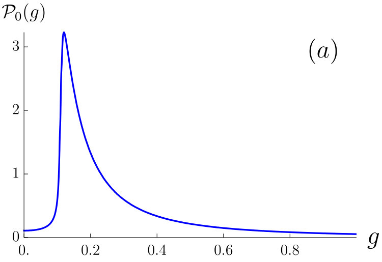 Figure 1
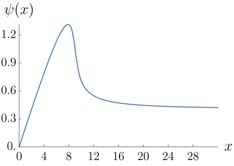 Figure 1
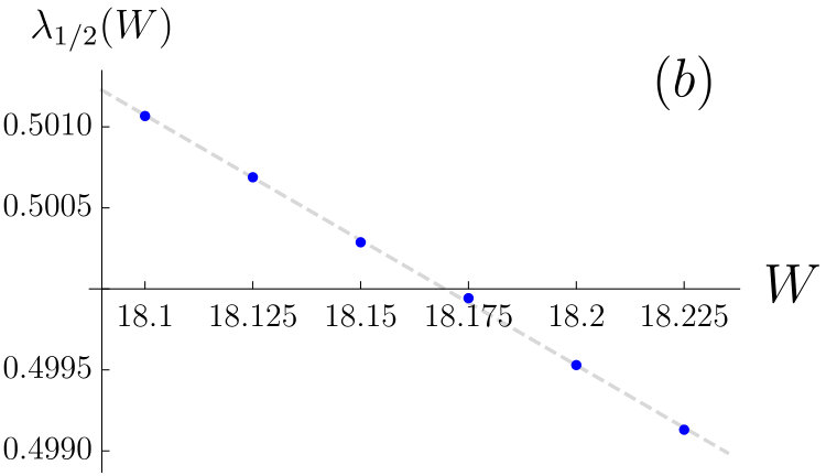 Figure 2
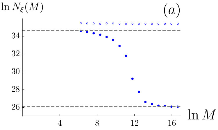 Figure 3
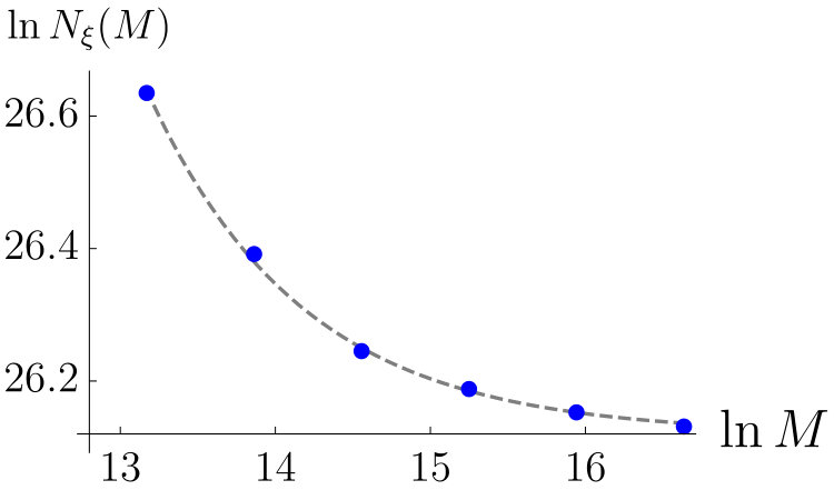 Figure 3
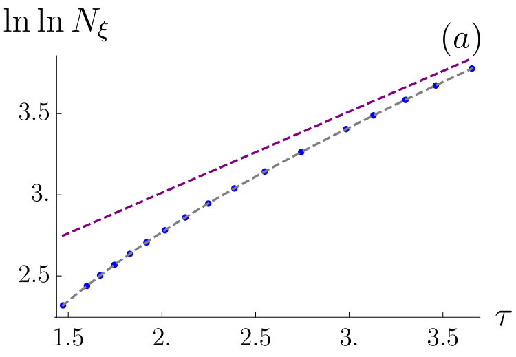 Figure 4
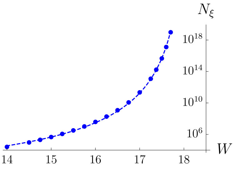 Figure 4
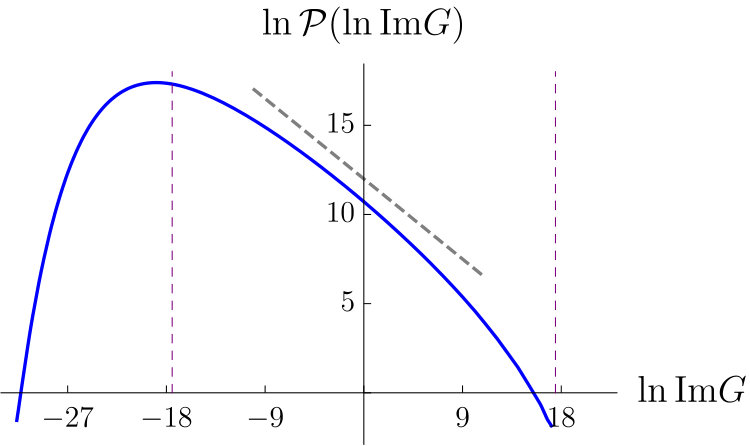 Figure 5
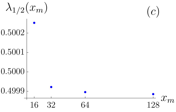 Figure 9
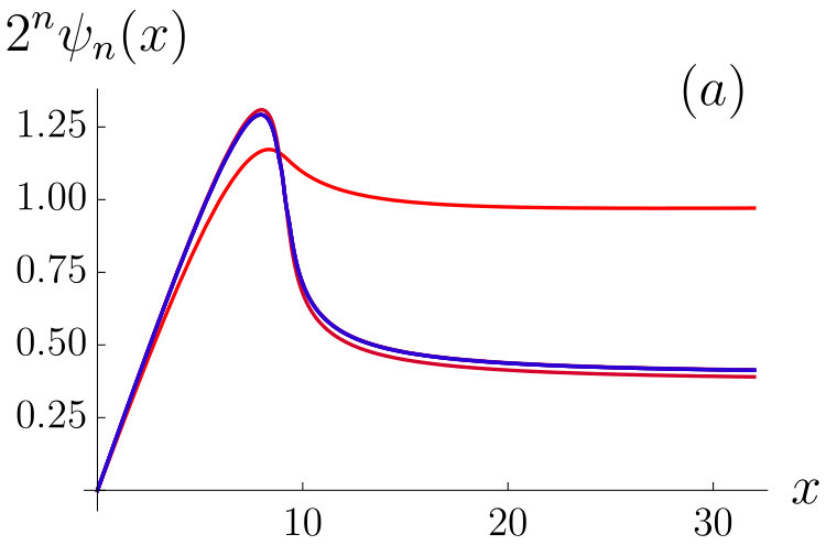 Figure 10
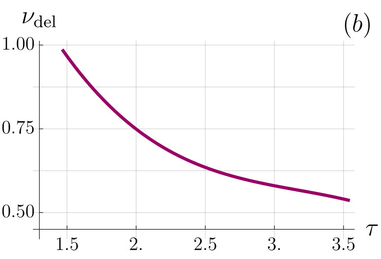 Figure 11
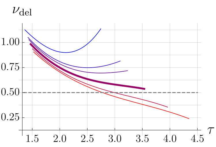 Figure 12
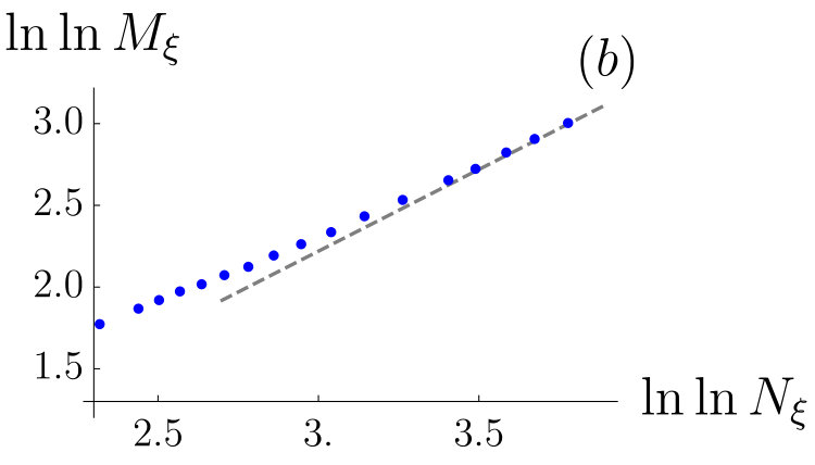 Figure 13
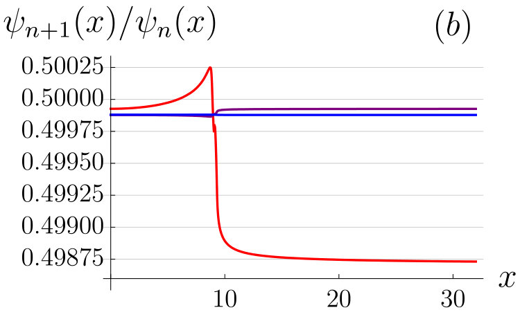 Figure 14
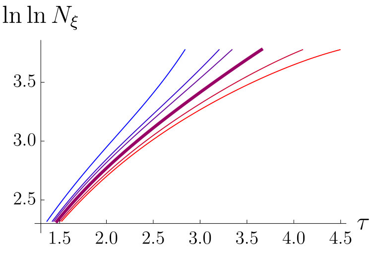 Figure 15
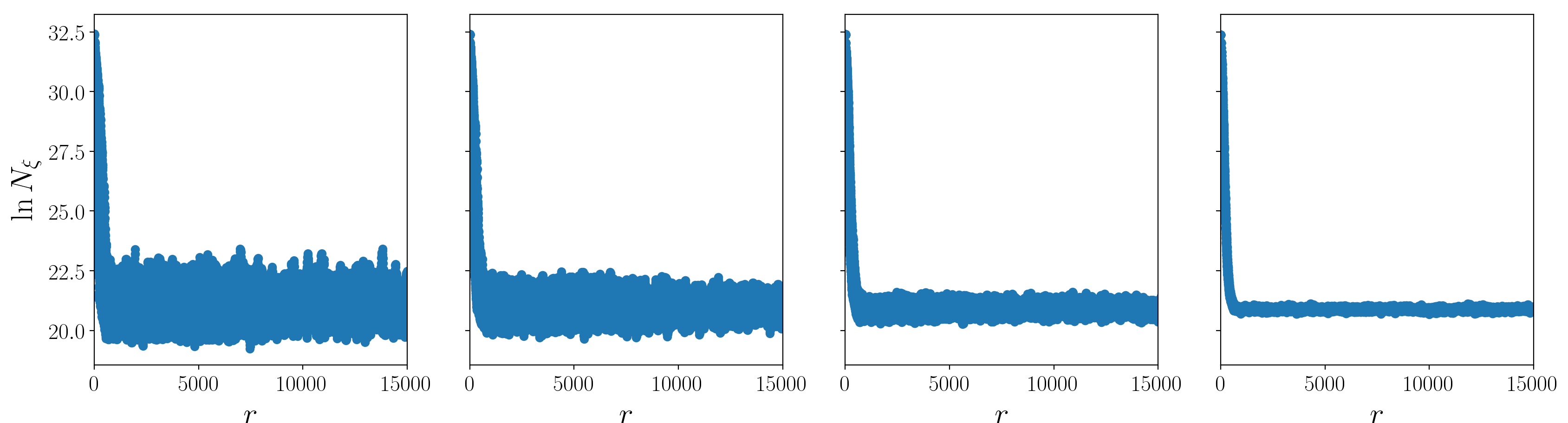 Figure 16
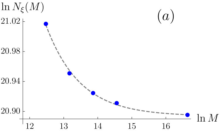 Figure 17
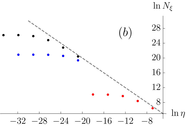 Figure 18
Peer Reviews
No public reviews on file for this paper yet. If you reviewed it on a platform where reviews are public (OpenReview, ICLR, NeurIPS, ICML), you can paste yours below so the community can read it here.
Videos
No videos yet. Explain this paper in a talk, walkthrough, or lecture? Add one.
Critical behavior at the localization transition on random regular graphs
K. S. Tikhonov
Institut für Nanotechnologie, Karlsruhe Institute of Technology, 76021 Karlsruhe, Germany
Condensed-Matter Physics Laboratory, National Research University Higher School of Economics, 101000 Moscow, Russia
L. D. Landau Institute for Theoretical Physics RAS, 119334 Moscow, Russia
A. D. Mirlin
Institut für Nanotechnologie, Karlsruhe Institute of Technology, 76021 Karlsruhe, Germany
Institut für Theorie der Kondensierten Materie, Karlsruhe Institute of Technology, 76128 Karlsruhe, Germany
L. D. Landau Institute for Theoretical Physics RAS, 119334 Moscow, Russia
Petersburg Nuclear Physics Institute,188300 St. Petersburg, Russia.
Abstract
We study numerically the critical behavior at the localization transition in the Anderson model on infinite Bethe lattice and on random regular graphs. The focus is on the case of coordination number , with a box distribution of disorder and in the middle of the band (energy ), which is the model most frequently considered in the literature. As a first step, we carry out an accurate determination of the critical disorder, with the result . After this, we determine the dependence of the correlation volume (where is the associated correlation length) on disorder on the delocalized side of the transition, , by means of population dynamics. The asymptotic critical behavior is found to be , in agreement with analytical prediction. We find very pronounced corrections to scaling, in similarity with models in high spatial dimensionality and with many-body localization transitions.
I Introduction
Anderson localization Anderson (1958) and, in particular, transitions between localized and delocalized phases Evers and Mirlin (2008) are among central themes of the condensed matter physics. Recently, there was a resurgence of interest to the Anderson models on random regular graphs (RRG) and on related tree-like graphs, largely in view of their relation to the Fock-space representation of interacting problems. Such relations have been pointed out for interacting quantum dot models Altshuler et al. (1997); Mirlin and Fyodorov (1997); Gornyi et al. (2017) as well as for many-body localization (MBL) problems with spatially localized single-particle states and short-range Gornyi et al. (2005); Basko et al. (2006); Gornyi et al. (2017) or long-range Gutman et al. (2016); Tikhonov and Mirlin (2018) interactions. The RRG ensemble is defined as that of random graphs with fixed coordination number (that is kept constant when one considers the limit of large number of sites ). A close relative of the Anderson model on RRG is the sparse random matrix (SRM) ensemble (also known as Erdös-Rényi graphs in mathematical literature) studied analytically in Refs. Mirlin and Fyodorov, 1991a; Fyodorov and Mirlin, 1991; Fyodorov et al., 1992. The central property of the RRG and SRM ensembles is that they represent tree-like models without boundary (and with loops of typical size ). The difference between the RRG and SRM models is that the connectivity is strictly fixed in the first case and is allowed to fluctuate in the second; this difference is inessential for the localization physics that we are interested in. In view of the connections to many-body problems mentioned above, one can view the Anderson model on RRG as a toy-model of MBL.
It was shown in Refs. Mirlin and Fyodorov, 1991a; Fyodorov and Mirlin, 1991; Fyodorov et al., 1992 that delocalized states in the SRM model have ergodic properties in the large- limit. These results were derived by means of a functional-integral representation of the correlation functions of the model in the framework of the supersymmetry formalism. In the large- limit, the integral can be evaluated by the saddle-point method. The corresponding saddle-point equation has a form analogous to the self-consistency equations obtained for the Anderson model Abou-Chacra et al. (1973); Mirlin and Fyodorov (1991b) and the model Efetov (1985); Zirnbauer (1986a, b); Efetov (1987a, b); Verbaarschot (1988) on an infinite Bethe lattice.
Numerical verification of the analytic predictions of Refs. Mirlin and Fyodorov, 1991a; Fyodorov and Mirlin, 1991; Fyodorov et al., 1992 turned out to be not so straightforward. In particular, the works Refs. Biroli et al., 2012; De Luca et al., 2014 questioned the ergodicity of the delocalized phase in the RRG model as defined by large- limit of the energy-level statistics and of scaling of the inverse participation ratio (IPR). Later, the analysis of Ref. Tikhonov et al., 2016 revealed a crossover from relatively small () to large () systems, where is the correlation volume. For the system exhibits a flow towards the Anderson-transition fixed point which has on RRG properties very similar to the localized phase. When the system volume exceeds , the direction of flow is reversed and the system approaches its ergodic behavior. The overall evolution with is thus non-monotonic. In combination with exponentially large values of the correlation volume , this makes the finite-size analysis very non-trivial. The main conclusions of Ref. Tikhonov et al., 2016 (in particular, the ergodicity of the delocalized phase) have been supported by subsequent studies of the IPR scaling in the SRM-like model García-Mata et al. (2017) and of the level number variance in the RRG model Metz and Castillo (2017), as well as in a recent extensive study of the RRG problem Biroli and Tarzia (2018). Further, we have recently performed Tikhonov and Mirlin (2019) a detailed analytical and numerical investigation of the level and eigenfunction statistics on RRG, both in the critical regime () and in the delocalized phase (). On the analytical side, we have extended the analysis of Refs. Mirlin and Fyodorov, 1991a; Fyodorov and Mirlin, 1991; Fyodorov et al., 1992 to the RRG model, in which case the saddle-point equation turns out to be identical to the self-consistency equation Abou-Chacra et al. (1973); Mirlin and Fyodorov (1991b) for the infinite Bethe lattice, and used it to calculate various observables. We have shown that these predictions, in combination with a numerical solution of the self-consistency equation, are in a perfect agreement with exact-diagonalization results for the eigenfunction and level statistics (in particular, for the IPR in the delocalized phase at ) on RRG.
As the saddle-point solution determines all physical observables on the RRG, it is important to understand its properties. This solution is intimately related to the distribution function of the local Green function on an infinite Bethe lattice Abou-Chacra et al. (1973); Mirlin and Fyodorov (1991b). The central role for the ergodicity of the extended phase on RRG (disorder , where is the Anderson-transition point) is played by the spontaneous symmetry breaking which manifests itself in the emergence of a non-zero typical value of the local density of states (LDOS) . Formally, the typical LDOS can be defined as , where denotes the disorder averaging. The typical LDOS on the infinite Bethe lattice is directly related to the correlation volume that is a key parameter characterizing the self-consistent solution in the delocalized phase, or, equivalently,
[TABLE]
Moments of on an infinite Bethe lattice are also determined by ; e.g.,
[TABLE]
As has been emphasized above, the scale controls the finite-size scaling of the RRG model: a not too large system, , behaves as critical, while for the ergodicity emerges. As an important example, the average IPR of eigenstates is of order unity for and is equal to
[TABLE]
for . It is worth emphasizing that the equality in Eq. (3) connects the IPR of states in the RRG model with fluctuations of the LDOS in the infinite-Bethe-lattice model Tikhonov and Mirlin (2019).
As for any phase transition, one of central questions is that of critical behavior near the transition point . On the delocalized side, it is particularly important to know the scaling of the correlation volume . As the linear size is proportional to the logarithm of the volume on a Bethe lattice (or RRG), it is natural to expect the scaling
[TABLE]
where the subscript “del” of the critical index indicates that we deal with the delocalized side of the transition. Indeed, the analysis of the Anderson model on an infinite Bethe lattice Mirlin and Fyodorov (1991b) yielded Eq. (4) with
[TABLE]
in analogy with earlier results for the model Zirnbauer (1986a); Efetov (1987a).
Numerical data of Refs. Tikhonov et al. (2016); García-Mata et al. (2017); Biroli and Tarzia (2018) for the RRG model were roughly consistent with this prediction, although an accurate determination of the correlation-volume scaling was not in the center of these studies. On the other hand, the value (5) of the critical index was questioned in Ref. Kravtsov et al. (2018) where both analytical and numerical arguments in favor of a different value, , were put forward.
In the present work, we resolve this question. The main subject of this work is a high-precision numerical analysis of the critical behavior of the scaling of the correlation volume . As a first step towards this goal, we accurately evaluate the critical disorder using the approach based on the stability analysis of Ref. Abou-Chacra et al. (1973). To simplify comparison with the previous literature, we choose the model that was studied in most of previous works (coordination number and box distribution of disorder). By carefully analyzing and eliminating numerical errors, we find , with an uncertainty less than . A precise knowledge of the critical point is very helpful for an accurate determination of the critical index, since otherwise should be used as an additional fitting parameter. Equipped in addition with large pool sizes (which allows us to approach closely), we are able to firmly establish the value of the critical index, , from the population-dynamics solution of the self-consistency equation. We also consider the form of the LDOS distribution near criticality and compare it to analytical prediction. In this connection, we also clarify the source of the error in the analytical argumentation of Ref. Kravtsov et al. (2018) with respect to the value of .
The structure of the paper is as follows. In Sec. II we define the Anderson models on an infinite Bethe lattice and on RRG to which our analysis applies. The critical disorder is determined numerically in Sec. III. In Sec. IV we explore the disorder dependence of correlation volume at the delocalized side of the transition and the determine the associated critical index, . Finally, Sec. V contains a summary of our results as well as a discussion of their connections to Anderson localization transitions in high spatial dimensionality and to MBL transitions.
II Model
The analysis of the correlation volume and of the self-consistent solution that we perform in this paper applies to two related models of non-interacting particles hopping over a graph with fixed connectivity in a potential disorder,
[TABLE]
where the sum is over the nearest-neighbor sites. The energies are independent random variables sampled from a distribution chosen as a box distribution, i.e., a uniform distribution on . We will study the models at zero energy, (i.e., in the middle of the band).
The first model is that of an infinite Bethe lattice Abou-Chacra et al. (1973); Mirlin and Fyodorov (1991b). In this model, the correlation volume , Eq. (4), characterizes the distribution of LDOS Mirlin and Fyodorov (1991b). To define the corresponding self-consistency equation, one has to introduce a small imaginary part of the energy. The symmetry breaking characterizing the delocalized phase implies that the distribution of LDOS has a non-singular limit at , which determines the value of the correlation volume under interest, see Eqs. (1) and (2). The notion of an infinite Bethe lattice corresponds to the limit taken before the limit .
The second model is the Anderson model on RRG. This model has by definition a finite (although large) number of sites . The observables of interest are statistical properties of eigenfunctions and of energy levels. As has been discussed in Sec. I, on the delocalized side of the transition, the critical volume marks a crossover from the critical regime, , to the ergodic behavior at Fyodorov and Mirlin (1991); Tikhonov et al. (2016); García-Mata et al. (2017); Biroli and Tarzia (2018); Tikhonov and Mirlin (2019). Furthermore, determines various properties of the delocalized phase at , including the coefficient in the ergodic () scaling of the IPR, Eq. (3), the spatial range of strong correlations in amplitudes of an eigenfunction, and the energy-level statistics beyond the random-matrix-theory regime Tikhonov and Mirlin (2019).
The self-consistency equation for the infinite Bethe-lattice model (or, equivalently, the saddle-point equation for the RRG model) can be presented in the form
[TABLE]
where the symbol denotes the equality in distribution for random variables. In this equation, has a meaning of the (advanced) Green function with coinciding spatial arguments, , defined on a slightly modified lattice, with the site 0 having only neighbors. On the right-hand-side of Eq. (7), are independent, identically distributed copies of the random variable and is a random variable with distribution . Equivalently, Eq. (7) can be written as a non-linear integral equation for the probability distribution of . We refer the reader to Eq. (4.6) of Ref. Abou-Chacra et al. (1973) and to Eqs. (17), (18) of Ref. Mirlin and Fyodorov (1991b) for two different representations of this equation; their equivalence is proven in Appendix C of Ref. Mirlin and Fyodorov (1991b).
Once the self-consistency equation is solved, one can calculate the distribution of the local Green function on an original lattice (with all sites having neighbors) from an auxiliary relation
[TABLE]
The distributions of and have qualitatively very similar properties. All the information about the position of the transition and the critical volume is contained in the self-consistency equation (7). Below we use short notations . We also focus on the case in the rest of the paper.
III Critical disorder
In this section, we perform an accurate evaluation of the critical disorder for the model with box distribution and coordination number . The strategy of finding the transition point was established in Ref. Abou-Chacra et al. (1973); equivalent results were later obtained within the supersymmetry formalism in Ref. Mirlin and Fyodorov (1991b). Very recently, the same equations were re-derived in Ref. Parisi et al. (2018). The procedure consists of two steps. First, one discards imaginary parts by setting and calculates the resulting distribution of real on-site Green functions . Then, one investigates the stability of this solution with respect to introducing a small imaginary part. This amounts to evaluating the largest eigenvalue of a certain integral operator, whose kernel involves . The stability (instability) implies that the system is in the localized (resp., delocalized) phase.
We begin with the first step. The distribution can be found from Eq. (7) at . The corresponding non-linear integral equation is Eq. (6.1) of Ref. Abou-Chacra et al. (1973) and Eq. (10) [or, equivalently, the unnumbered equation preceding Eq. (23)] of Ref. Mirlin and Fyodorov (1991b).
A standard approach for solving equations such as Eq. (7) is population dynamics, also known as pool method. With a given pool size , we iterate the self-consistency equation (with ) until convergence. As a result we get a sample of variables distributed according to and recover the distribution function binning the data and interpolating the resulting counts. The result is shown in Fig. 1a for ; since is an even function of , we show it only for . The distribution has a relatively sharp peak at , which is a consequence of the box distribution with the border at the energy . Further, very generally, has a power-law tail, at , where is the average DOS.
Having evaluated , we turn to the second step. Upon introduction of a small level broadening (imaginary part of the energy), the Green function becomes complex, and one has to study the joint distribution . The distribution of imaginary part, , may have either regular or singular limit at . The first case (i.e., spontaneous emergence of a non-trivial distribution of ) corresponds to the delocalized phase, the second case to the localized phase. The transition between these two types of behavior happens at , which is a point of the localization transition. In order to find , one studies the stability of the localized phase, i.e., of the distribution with purely real . The latter is stable if and only if the largest eigenvalue of the linear integral operator with the kernel
[TABLE]
is smaller than for . For purpose of brevity, we have written the kernel in Eq. (9) for the particular case . The general form (valid for arbitrary ) of the operator can be found in Eq. (6.5) of Ref. Abou-Chacra et al. (1973) and in Eq. (26) of Ref. Mirlin and Fyodorov (1991b).
One should therefore study the eigenvalue problem
[TABLE]
The spectrum and eigenfunctions of this equation evolve smoothly as functions of disorder. One way to study Eq. (10) would be to discretize operator in Eq. (9) Parisi et al. (2018). However, since the kernel of this equation as well as the solution vary steeply in certain regions of arguments (see Fig. 1), it is very difficult to find the eigenvalue with high accuracy in this manner, unless the mesh is chosen very carefully. We prefer to solve Eq. (9) iteratively,
[TABLE]
choosing the adaptive mesh at each step of the iterative procedure, so that accuracy of the representation is kept above certain predefined threshold. In order to further improve the accuracy, we use the following asymptotic formula:
[TABLE]
which follows from Eqs. (9), (11). In our iterative scheme, we employ this equation by introducing a parameter such that for the function is represented by the asymptotic tail (12) with coefficient chosen to match the known value of to the calculated points at . The value of is chosen in such a way that the eigenvalue is found with sufficient accuracy (see below).
In the end, we aim to obtain with 4 significant digits. It turns out that the largest eigenvalue of the operator strongly dominates all others, so that 6 iterations are sufficient to find this eigenvalue to the desired accuracy (see Figs. S1a,b in Supplemental Material where we show found from repeated application of the recursive equation). The corresponding eigenfunction for is shown in the inset of Fig. 1a.
In order to find the critical point, we perform the described procedure for several values of in the range ; the results are shown in Fig. 1b. Solving the equation (with ), we find
[TABLE]
To understand the accuracy of the result, it is important to analyze possible sources of errors. Formally, we perform all computations (integrations and interpolations) so that at least 6 digits of the result are expected to be correct. However, the method of the calculation itself has several parameters, finiteness of which is the source of a systematic error: i) the pool size , ii) the histogram bin size , iii) the cutoff beyond which the function is replaced by its tail, and iv) the parameter beyond which the asymptotic formula (12) is used. Statistical error of the result is due to fluctuations of the bin counts and is controlled by the number of realizations of the pools (we have from to independent samples for from to ). We have evaluated for a set of parameters and found that upon varying them in a wide range foo , evolves only in the 5th digit. (In particular, we observe a dependence on the pool size in the range which is at least two orders of magnitude weaker than that of Ref. Parisi et al. (2018)). The most important source of a systematic error is (see Supplemental Material, Fig. S1c for the corresponding dependence), and in the final calculation we use . We thus conclude that the value of the has an absolute precision of . This translates into the uncertainty in less than . Thus, the estimated uncertainty of our result is within .
It is interesting to compare this accurate value of with previous numerical results obtained for the same model. The first such calculation was performed in the pioneering paper Abou-Chacra et al. (1973) and yielded an estimate . Subsequent works yielded improved estimates Monthus and Garel (2008), and Biroli et al. (2010) (improvements were mostly related to increasing the pool size). Recently, three papers aimed for a more accurate determination of and found Biroli and Tarzia (2018), Kravtsov et al. (2018), and Parisi et al. (2018). As we will demonstrate in the next section, such deviations are actually very strong in the context of determination of the critical behavior, so it is important to understand the origin of the controversies. The value found in Ref. Biroli and Tarzia (2018) has larger uncertainty than our result, and within this uncertainty it is consistent with our Eq. (13). The values found in Ref. Parisi et al. (2018) and especially in Ref. Kravtsov et al. (2018) deviate more sizeably from our result. The analysis of Ref. Parisi et al. (2018) that yielded has probably suffered from a not sufficiently accurate solution of Eq. (10) caused by fixed mesh discretization. As to Ref. Kravtsov et al. (2018), we believe that errors in numerical determination of resulted from a combination of several sources. First, contrary to our approach, in which we first determine with high accuracy and then study the critical behavior, the authors of Ref. Kravtsov et al. (2018) attempted to do this simultaneously, which is less favorable from the point of view of the accuracy in the presence of large corrections to scaling [see discussion after Eq. (27)]. Second, the corresponding analysis was not carried out in Ref. Kravtsov et al. (2018) in an optimal way (see Fig. S4 and the associated comments in Supplemental Material). Finally, determination of in this work appears to be plagued by sizeable numerical errors. Apparently, the authors relied on points derived for insufficiently small too close to criticality: the smallest value of that is quoted in the caption to Fig. 8 of Ref. Kravtsov et al. (2018), , is way too large, as the studied correlation volumes exceed at .
IV Delocalized phase
With an accurate value of at hand, see Eq. (13), we turn to the analysis of the critical behavior in the delocalized phase. As has been already discussed above, the solution is unstable at to introduction of finite . In the field-theoretical description of the Anderson localization, this phenomenon can be cast in the framework of spontaneous symmetry breaking, with an order-parameter function intimately related to the distribution of LDOS. As a result, a non-trivial distribution emerges, which can be found from a complex-valued pool method applied to Eqs. (7), (8).
The population dynamics calculation is conducted at a finite (although large) pool size and a finite (although small) imaginary part of the energy, . The resulting distribution can be characterized by “effective correlation volume” defined as the population-dynamics result for , where includes averaging over many iterations after the approximate convergence is reached. It is obvious that at finite the distribution of sampled by iterative procedure is not exactly that of limit. One can expect that for smaller pool sizes the sample-to-sample fluctuations of the typical value of are large and decrease with growing . This is indeed the case, see Fig. S2 of Supplemental Material for illustration of the evolution of the iterative procedure with increasing . As soon as is large enough, these fluctuations mostly average out and the result is weakly dependent on . In the end, the true correlation volume is given by the double limit
[TABLE]
To illustrate the role of the pool size, we show in Fig. 2a the dependence of on for and fixed . It is seen that for relatively small pool sizes is essentially equal to , which is a characteristic behavior for the localized phase and the critical point. With increasing , the system “recognizes” that it is actually on the delocalized side of the transition, and crosses over to the value . If has been chosen to be sufficiently small, , the behavior of at large is essentially independent on , i.e., (see Fig. S3b in Supplemental Material for more detail). The limiting value yields the sought physical correlation volume . This behavior in the delocalized phase should be contrasted to the data for the localized side of the transition, , which illustrate the stability of the localized phase with respect to .
We find that the large- approach of to its asymptotic value is rather fast and is very well fitted by the dependence:
[TABLE]
see the inset of Fig. 2a as well as Fig. S3a of Supplemental Material. We obtain this asymptotic behavior for all studied values of . The parameter in Eq. (15) defines the pool size that is needed to obtain up to a factor of order unity. In Fig. 2b we have shown as a function of , with a double-logarithmic scale on each axis. A natural expectation would be that is of the order . Indeed, we observe a unit asymptotic slope of the dependence in Fig. 2b, which implies that has the same asymptotic behavior (4) as , with the same exponent . On the other hand, there is also a non-trivial intercept,
[TABLE]
which means that
[TABLE]
with . In other words, the pool size needed to find accurately is in fact much smaller than , although it diverges at in the same exponential fashion.
The disorder dependence of the correlation volume obtained according to Eq. (14) is shown in Fig. 3a. More specifically, we plot as a function of . In this representation, the asymptotic slope , where
[TABLE]
yields the sought index in the critical behavior (4) of the correlation volume. In Fig. 3b, we show the dependence of the slope , which can be viewed as a “flowing critical index”. It is seen that decreases substantially with increasing and saturates at . The found saturation value is in a perfect agreement with the analytical prediction , Eq. (5). We thus have numerically determined the critical behavior of the correlation volume , or, equivalently, of the corresponding correlation length ,
[TABLE]
In fact, the analytical theory predicts not only the critical index of the scaling (19) of but also the corresponding numerical prefactor. The analysis of the symmetry-broken solution near in the Anderson model Mirlin and Fyodorov (1991b) model bears (in analogy with its model counterpart Zirnbauer (1986a); Efetov (1987a)) a close connection to the analysis of stability of the localized phase. It leads to the equation
[TABLE]
where is the largest eigenvalue of the operator (9). We recall that in our case. Expanding the eigenvalue around and up to the leading non-vanishing terms, we get
[TABLE]
For below , the solution of Eqs. (20), (21) is
[TABLE]
The imaginary part determines, via the equation Mirlin and Fyodorov (1991b)
[TABLE]
the correlation volume . Evaluating numerically the largest eigenvalue of operator in Eq. (9) for close to 1/2 and close to , we find
[TABLE]
Substituting these values in Eqs. (22), (23), we finally get the numerical value of the prefactor in the asymptotic scaling law for ,
[TABLE]
This asymptotic expression is shown in Fig. 3a by magenta dashed line. The agreement between the population-dynamics results and this analytical prediction for the asymptotic behavior is very impressive.
It is instructive to compare these exact results with the large- approximation. This approximation is formally valid for (since is proportional to for large ); we will see, however, that it works very well already for (which is related to the numerically quite large value ). For large , the eigenvalue is given by the asymptotic formula Tikhonov and Mirlin (2016)
[TABLE]
Substituting this formula in Eq. (20) with , one finds the corresponding approximation for the critical disorder . For , this gives , which differs only by from the exact result . Further, expanding Eq. (26) with respect to and , see Eq. (21), and substituting the corresponding coefficients and in Eqs. (22), (23), we getmf
[TABLE]
For , this equation yields , thus reproducing the correct numerical coefficient in Eq. (25) with amazing accuracy of .
Let us emphasize the following important point. The fact that saturates at a non-trivial value (actual critical index ) at is a consequence of the correct choice of the critical point, , in the definition of . If we would use a lower value of , the resulting dependence would tend to zero at , since we would reach infinite while being still in the delocalized phase. By similar token, taking larger than the actual value, we would get increasing tending to diverge at a finite . This is illustrated in Fig. S4 of Supplemental Material, where we compare the correct () with dependencies obtained by using smaller (, ) and larger (, and ) values of tentative in the definition of . The expected behavior is clearly seen, so that, solely on the basis of the data for , we could conclude that is in the range – . (Note that the value proposed in Ref. Kravtsov et al. (2018) is well outside this range; see Supplemental Material for more comments on a deficiency of the numerical procedure in that work.) As has been already emphasized, the accuracy of this method of determination of is significantly lower than of that based on investigation of stability of the localized phase, Sec. III. At the same time, the agreement between the two approaches is encouraging.
The population-dynamics analysis provides not only but also the full distribution of the Green function . In Fig. 4 we illustrate the distribution of the imaginary part ; this is essentially the distribution of LDOS . As expected, we observe the power-law distribution
[TABLE]
outside of this range the probability is strongly suppressed. This behavior of is essentially the same as the one found in the model on the Bethe lattice Mirlin and Fyodorov (1994a, b). The LDOS distribution (28) is intimately related to the eigenvalue in Eq. (22). Specifically, the real part 1/2 of translates into the exponent 3/2 in the LDOS distribution (28), while the imaginary part determines, via the equation (23), the correlation volume which controls the range of validity of the power-law distribution (28).
At this point, it is appropriate to comment on the error in the analytical argument of Ref. Kravtsov et al. (2018) that suggested an incorrect value of the exponent, . The authors of this paper did not appreciate a difference in the LDOS statistics in the models of infinite and finite Bethe lattices. (In the first the case the limit is taken before the limit ; in the second case the order of limits is opposite.) This difference has been demonstrated in great detail in Ref. Tikhonov and Mirlin (2016) where the statistics of eigenfunctions and LDOS at a root of the finite Bethe lattice was studied. In particular, the parameter of Ref. Kravtsov et al. (2018) is the parameter of Ref. Tikhonov and Mirlin (2016) that characterizes the fractal statistics on a finite Bethe lattice. This parameter changes linearly as a function of disorder near , which apparently leads to the value deduced by Ref. Kravtsov et al. (2018), see Eqs. (56)-(60) of that work. The argument is incorrect since the parameter of Ref. Tikhonov and Mirlin (2016) (i.e., of Ref. Kravtsov et al. (2018)) applies to a finite Bethe lattice but not to the infinite one. This error is closely related to a more general deficiency of Ref. Kravtsov et al. (2018) that fails to properly discriminate between the fractal properties on a finite Bethe lattice and the ergodicity of the delocalized phase on RRG.
It is worth emphasizing that the critical index that we have studied in this paper characterizes the correlation length on the delocalized side of the transition, . The counterpart of on the localized side, , is the localization length that is a length controlling the exponential decay of the density-density correlation function (multiplied by the factor ) with the distance . This length is given by Mirlin and Fyodorov (1991b)
[TABLE]
and scales near the critical point as
[TABLE]
in analogy with the corresponding results for the model Zirnbauer (1986a); Efetov (1987a). The different scaling of the characteristic lengths on both sides of the transition is a special feature of the Bethe-lattice and RRG models, distinguishing them from the conventional dimensional models. We also mention that, on the delocalized side of the transition, further two lengths (much larger than ) were identified that control the asymptotic decay of the connected part of a LDOS-LDOS correlation function and scale with indices 1 and 3/2 Zirnbauer (1986a); Efetov and Viehweger (1992). These lengths appear to be, however, of minor physical importance for the physics of the RRG model. Indeed, it is the length (or, equivalently, the correlation volume ) that determines the finite-size crossover from the critical regime to the ergodic behavior on RRG, thus controlling the associated scaling properties of wave-function and energy level statistics and of further related observables Tikhonov and Mirlin (2019).
V Summary
To summarize, we have studied numerically the critical behavior at the localization transition in the Anderson model on infinite Bethe lattice and on RRG. We have focused on the case of coordination number , with a box distribution of disorder and in the middle of the band, , which is the model most frequently considered in the literature. As a first step, we have carried out an accurate determination of the critical disorder , carefully analyzing all essential sources of numerical errors. The resulting value is . After this, we have determined the dependence of the correlation volume on disorder on the delocalized side of the transition, . This analysis was done by means of population dynamics, with pool sizes up to , and with obtained as , where is the one-site Green function and is the LDOS (times ). Also in this part of the study, we have carefully analyzed convergence with respect to all relevant parameters, including the pool size, the number of iterations, and the imaginary part of the energy. The resulting dependence is shown in Fig. 3a. In view of the relation between the RRG model and that on the infinite Bethe lattice, which was established analytically Mirlin and Fyodorov (1991a); Fyodorov and Mirlin (1991); Tikhonov and Mirlin (2019) and confirmed numerically Tikhonov and Mirlin (2019), the obtained correlation volume also characterizes the RRG problem in which it controls a crossover from criticality to ergodicity.
It is worth emphasizing that we were able to reach controllably values of the correlation volume as large as , which is many orders of magnitudes larger than the volume of a system that one could study directly (via exact diagonalization). This is because the problem allows to use the population-dynamics approach. First, the maximal pool size that we employ is , which is already much larger than the size of a system that can be diagonalized. In addition to this, and quite remarkably, the correlation volume that can be reached turns out to be much larger than the pool size , see Fig. 2b and Eq. (16).
With the accurate value of and the dependence of at hand, we have determined numerically the critical index of the correlation length . For this purpose, we have plotted the flowing exponent , see Fig. 3b. The true exponent is given by the limit . The numerically established decreases monotonically and saturates at large . The saturation value is in a good agreement with the analytical prediction , Eq. (19). A substantial (factor-of-two) variation of the “running exponent” in Fig. 2 serves as an indication of rather appreciable corrections to scaling, which underlines the importance of proceeding within our analysis up to such large .
Numerical evaluation of critical indices for non-interacting Anderson transitions was a subject of very intense activity over a few decades. As an example, let us focus on the “standard model” of the Anderson transition—that for a 3D system in the orthogonal universality class. Development of the finite-size-scaling approach has allowed one to determine the exponent of the localization (correlation) length as MacKinnon (1983). Subsequent works have increased the accuracy and rederived the exponent by several complementary approaches Varga (1995); Zharekeshev (1997); Slevin (1999); Milde (2000); Rodriguez et al. (2010); Slevin and Ohtsuki (2014, 2018). In particular, a recent resultSlevin and Ohtsuki (2018) is , which means an amazingly high precision of in determination of the critical index. One thus might be surprised that a comparable numerical analysis of scaling has not been done long ago also for Anderson models on the Bethe lattice and on RRG. This is related to a much higher computational complexity of the RRG model in comparison to its 3D counterpart. The reasons for this are twofold. First, the volume on RRG (or on the Bethe lattice) is an exponential function of length , . As an illustration, the huge correlation volume (our largest value) on RRG corresponds to the correlation length that does not look so large from the point of view of a 3D system. Second, corrections to a “simple” one-parameter scaling are much more pronounced for RRG than for a 3D Anderson transition. As a manifestation of this, any scaling analysis for the RRG model is severely complicated by the fact that the crossing point for finite-site scaling curves (-dependencies of some observable for different fixed ) drifts strongly with Tikhonov et al. (2016). In fact, a trend towards such a behavior has been also observed in the analysis of the Anderson transition -dimensional systems with Zharekeshev (1998); Markoš (2006); García-García and Cuevas (2007); Ueoka and Slevin (2014); Tarquini et al. (2017); it becomes particularly pronounced for the largest studied value . Another manifestation of large corrections to scaling is a strong variation of the flowing exponent , see Fig. 3b.
Since the RRG model realizes, in a certain sense, a limit of the Anderson transition, one can wonder whether a “symmetric” scaling (the same exponent on both sides) in a finite is not in conflict with an “asymmetric” scaling () on RRG. The resolution is that the range of validity of the symmetric scaling around the critical disorder gradually shrinks towards zero with increasing dimensionality, .
As has been mentioned in Sec. I, the RRG model can be viewed as a toy-model for the MBL transition. Let us briefly discuss the known numerical results for the scaling near the MBL transition (which were mainly obtained for interacting 1D spin chains with disorder in the form of a random Zeeman field Oganesyan and Huse (2007); Kjäll et al. (2014); Nandkishore and Huse (2015); Luitz et al. (2015); Serbyn et al. (2015); Geraedts et al. (2017); Khemani et al. (2017); Abanin and Papić (2017); Doggen et al. (2018); Macé et al. (2018)) and compare them to the Anderson transition on RRG. The two types of transitions show indeed a great deal of similarity. The tentative position of the MBL transition as derived from the data for systems of size moves strongly towards larger disorder, in full similarity with RRG. The critical point of the MBL transition appears to show, in many respects, properties of the localized phase, also in similarity with RRG. Furthermore, the critical indices that have been found by numerical scaling analysis of the MBL transition are in the range Kjäll et al. (2014); Luitz et al. (2015); Macé et al. (2018). This shows again a similarity with the RRG transition, for which the index on the localized side is and on the delocalized side , with finite-size effects in small systems leading to an apparent increase of the latter value, see Fig. 3b. We note that the above values are in a strong conflict with Harris criterion , so that they cannot be the true asymptotic exponents for the MBL transition. The tentative resolution of this apparent contradiction is that the true asymptotic behavior shows up only in very large systems Chandran et al. (2015). Thus, systems of moderate sizes (relevant to experiments) may exhibit the behavior akin to that in the RRG model. (See Ref. Tikhonov and Mirlin (2018) for “translation” of the RRG critical behavior to that with respect to the spatial length ; for the dimensionality this does not modify the exponents.)
What are further lessons that results of the present work teach us in connection with investigation of the scaling at MBL transitions? First, the exponents controlling the finite-size scaling in the RRG problem are different on both sides of the transition ( vs. ). It is quite likely that the same property is relevant to the MBL transition as well. On the other hand, most of the previous analysis of numerical data around the MBL transition Kjäll et al. (2014); Luitz et al. (2015) has assumed equal exponents on both sides. Very recently, a scaling analysis with different exponents has been carried out Macé et al. (2018), with the results and quite similar to the RRG values. A more detailed study of this “asymmetry” of the critical behavior at the MBL transition would be of great interest. Second, taking into account corrections to scaling is of crucial importance for proper analysis of this class of localization transition. Third, the accuracy of the numerical study of the transition in the present work was greatly favored by the possibility to apply the population-dynamics approach. As has been already emphasized above, this has allowed us to increase the maximal effective system size from 20 (characteristic for the exact-diagonalization study) to more than 60. Key to this progress in the study of the RRG transition was the relation to the infinite-Bethe-lattice model arising in the framework of the field-theoretical analysis. It would be important to see whether any more realistic MBL model allows for a similar treatment. Finally, our observation that is sufficient to reach the asymptotic behavior with a very reasonable accuracy (at least for the RRG model) is encouraging from the point of view of experimental studies of the MBL problems (for a recent review see Ref. Abanin et al. (2018)). Indeed, the reported experimental realizations with cold-atom systems contained about 100 of atoms Choi et al. (2016); Schreiber et al. (2015). Further, quantum simulators with particles based on Rydberg states of trapped cold atoms Bernien et al. (2017) and on trapped ions Smith et al. (2016) have been reported; such or related systems can also serve for the investigation of the MBL transition.
Finally, one foresees that quantum computers with 50-100 qubits will be available in a not so far future Kelly et al. (2019). One can thus expect important results on critical properties near the MBL transition (even if describing only some intermediate regime) provided by quantum computations and simulations in the next few years. It is worth mentioning that the study of statistical properties of states on the ergodic side of the MBL transition has much in common with the problem of sampling from complex distributions that is an indicator of quantum supremacy that is expected to be reached when the number of qubits exceeds 48 Boixo et al. (2018).
VI Acknowledgments
We are grateful to M. V. Feigel’man for useful discussions and A. Scardicchio for attracting our attention to preprint Parisi et al. (2018). This work is supported by the program 0033-2019-0002 by the Ministry of Science and Higher Education of Russia. KT acknowledges support by Alexander von Humboldt Foundation.
The reference list from the paper itself. Each links out to its DOI / PubMed record.
- 1Anderson (1958) P. W. Anderson, Physical Review 109 , 1492 (1958).
- 2Evers and Mirlin (2008) F. Evers and A. D. Mirlin, Reviews of Modern Physics 80 , 1355 (2008).
- 3Altshuler et al. (1997) B. L. Altshuler, Y. Gefen, A. Kamenev, and L. S. Levitov, Physical Review Letters 78 , 2803 (1997).
- 4Mirlin and Fyodorov (1997) A. D. Mirlin and Y. V. Fyodorov, Physical Review B 56 , 13393 (1997).
- 5Gornyi et al. (2017) I. Gornyi, A. Mirlin, D. Polyakov, and A. Burin, Annalen der Physik 529 (2017).
- 6Gornyi et al. (2005) I. Gornyi, A. Mirlin, and D. Polyakov, Physical Review Letters 95 , 206603 (2005).
- 7Basko et al. (2006) D. Basko, I. Aleiner, and B. Altshuler, Annals of Physics 321 , 1126 (2006).
- 8Gutman et al. (2016) D. B. Gutman, I. V. Protopopov, A. L. Burin, I. V. Gornyi, R. A. Santos, and A. D. Mirlin, Physical Review B 93 , 245427 (2016) . · doi ↗