Lead Geometry and Transport Statistics in Molecular Junctions
Michael Ridley, Emanuel Gull, Guy Cohen

TL;DR
This paper uses the Inchworm quantum Monte Carlo method to study charge transport and fluctuations in molecular junctions, highlighting how lead geometry and finite bandwidth influence transport properties beyond traditional models.
Contribution
It demonstrates the application of a numerically exact technique to analyze lead geometry effects and reveals interaction-induced broadening of transport channels in molecular junctions.
Findings
Finite lead bandwidth affects transport properties.
Current fluctuations are more sensitive probes than mean current.
Interaction-induced broadening is visible at all voltages.
Abstract
We present a numerically exact study of charge transport and its fluctuations through a molecular junction driven out of equilibrium by a bias voltage, using the Inchworm quantum Monte Carlo (iQMC) method. After showing how the technique can be used to address any lead geometry, we concentrate on one dimensional chains as an example. The finite bandwidth of the leads is shown to affect transport properties in ways that cannot be fully captured by quantum master equations: in particular, we reveal an interaction-induced broadening of transport channels that is visible at all voltages, and show how fluctuations of the current are a more sensitive probe of this effect than the mean current.
Click any figure to enlarge with its caption.
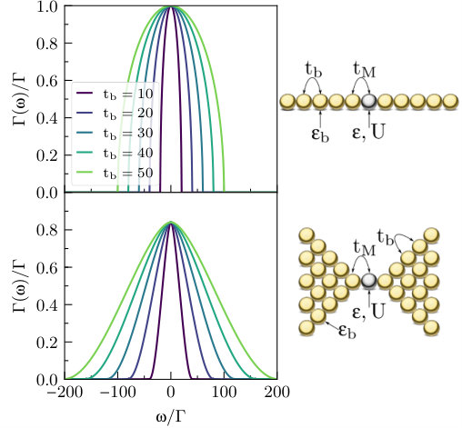 Figure 1
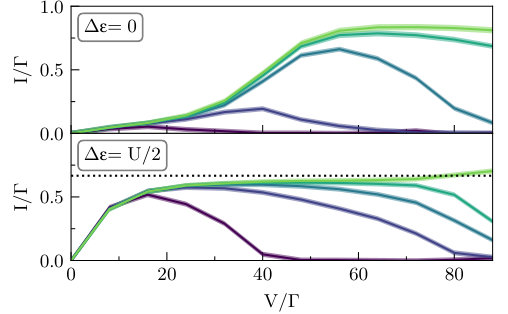 Figure 2
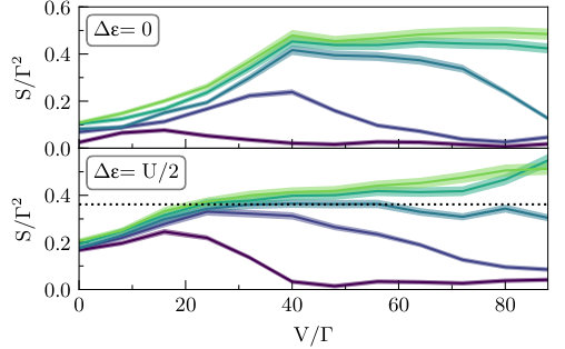 Figure 3
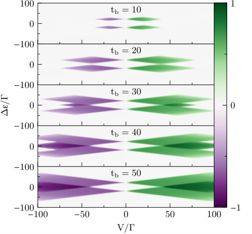 Figure 4
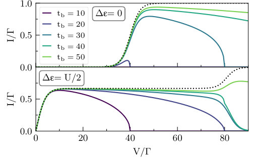 Figure 5
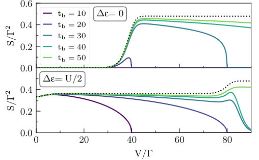 Figure 6
Peer Reviews
No public reviews on file for this paper yet. If you reviewed it on a platform where reviews are public (OpenReview, ICLR, NeurIPS, ICML), you can paste yours below so the community can read it here.
Videos
No videos yet. Explain this paper in a talk, walkthrough, or lecture? Add one.
Lead Geometry and Transport Statistics in Molecular Junctions
Michael Ridley
School of Chemistry, Tel Aviv University, Tel Aviv 69978, Israel
The Raymond and Beverley Sackler Center for Computational Molecular and Materials Science, Tel Aviv University, Tel Aviv 6997801, Israel
Emanuel Gull
Department of Physics, University of Michigan, Ann Arbor, Michigan 48109, USA
Center for Computational Quantum Physics, Flatiron Institute, New York, New York 10010, USA
Guy Cohen
School of Chemistry, Tel Aviv University, Tel Aviv 69978, Israel
The Raymond and Beverley Sackler Center for Computational Molecular and Materials Science, Tel Aviv University, Tel Aviv 6997801, Israel
Abstract
We present a numerically exact study of charge transport and its fluctuations through a molecular junction driven out of equilibrium by a bias voltage, using the Inchworm quantum Monte Carlo (iQMC) method. After showing how the technique can be used to address any lead geometry, we concentrate on one dimensional chains as an example. The finite bandwidth of the leads is shown to affect transport properties in ways that cannot be fully captured by quantum master equations: in particular, we reveal an interaction-induced broadening of transport channels that is visible at all voltages, and show how fluctuations of the current are a more sensitive probe of this effect than the mean current.
I Introduction
The conductance properties of single molecule junctions paint a rich picture of the internal dynamics of open quantum systems far from equilibrium. However, electron transport through a molecule coupled to conducting leads at finite temperature is inherently stochastic,(Blanter and Büttiker, 2000) and fluctuations in the current can provide a great deal more information than the conductance or current alone.(Esposito et al., 2009) The current, its fluctuations or noise, and higher-order statistical cumulants can be obtained from the so-called full counting statistics (FCS) approach.(Levitov and Lesovik, 1993; Levitov et al., 1996) In recent years, noise and FCS techniques have been used to understand many physical properties in both experimental and theoretical transport settings. A few examples are quasiparticle charges in nanotube junctions;(Ferrier et al., 2016, 2017) magnetic effects, channel determinations and thermotransport in atomic junctions;(Vardimon et al., 2013; Kumar et al., 2013; Vardimon et al., 2016; Lumbroso et al., 2018) waiting time(Albert et al., 2011; Kosov, 2017) and first passage time(Ridley et al., 2018) distributions; correlations between currents in different leads;(Ridley et al., 2017) thermodynamic efficiency fluctuations;(Esposito et al., 2015) and fluctuation–dissipation relations.(Nakamura et al., 2010; Küng et al., 2012; Pekola, 2015)
The treatment of noninteracting electron transport and FCS is at an advanced stage, and both analytical and numerical methods are available.(Levitov and Lesovik, 1993; Büttiker, 1986; Croy and Saalmann, 2009; Tang and Wang, 2014; Ridley et al., 2015) However, the inclusion of many-body interactions in even the simplest impurity models, where a small interacting impurity or molecule is coupled to large noninteracting leads, remains theoretically challenging. A variety of numerical approaches exists, each with different advantages and disadvantages depending on the particular model in question and the physical parameters. These might include, e.g., a lead–molecule coupling strength , a temperature , an applied voltage and a local Coulomb interaction strength .
In addition to this set of discrete energy scales, molecular conductance also depends strongly on the geometry of the leads and the nature of the coupling between the lead and the molecule, a phenomenon which is often studied theoretically in the context of noninteracting(Feng et al., 2008; Yang et al., 2014; Zelovich et al., 2015) and weakly correlated(Darancet et al., 2012) systems. Transport experiments show large variation of conductance with the respect to the detailed structure of the lead–molecule interface, in particular the chemistry of the anchoring group at the interface.(Zotti et al., 2010; Venkataraman et al., 2006; Quek et al., 2007; Hong et al., 2012) However, in simplified theoretical treatments, and especially when dealing with many-body systems, it is often convenient to neglect the internal electronic structure of the leads. One common assumption is the wide band limit approximation.(Nitzan, 2006; Ridley et al., 2017) Assuming a finite lead bandwidth is perhaps the simplest concession to experimental reality that might be made, and is enough to show that a strong effect on transport exists even in the non-interacting case.(Oz et al., 2018) A more general approach for interacting systems is therefore highly desirable.
In the regime of small lead–molecule coupling and high temperatures, the quantum master equation (QME) method offers a fast and elegant means for investigating the basic conduction properties(Harbola et al., 2006; Esposito and Galperin, 2010) and FCS(Bagrets and Nazarov, 2003; Kießlich et al., 2006) of molecular junctions. The basic Lindblad or Redfield QME approaches assume Markovian dynamics, thus neglecting memory effects due to finite bandwidth and lead structure. Most QME methods are also perturbative in the molecule–bath coupling, and thus restricted to low-order effects like sequential tunneling. More advanced generalizations of the QME method include, for example, non-Markovian memory effects(Flindt et al., 2008) and inelastic cotunneling processes.(Kaasbjerg and Belzig, 2015) Novel formulations more loosely connected to the QME even allow for the approximate treatment of strong correlations, and may also include the effects of external driving fields.(Dou et al., 2017, 2018) Equation of motion approaches, also loosely related, can be formulated so as to correctly capture the noninteracting limit(Zubarev, 1960; Levy and Rabani, 2013a, b; Levy et al., 2019); and other approaches are exact at the semiclassical limit.(Swenson et al., 2011, 2012) Still, many of these approximations lack some of the advantages of more naive QME approaches, which may result, e.g., in the violation of the positivity of the density matrix(Breuer et al., 2002) or a failure to satisfy various detailed balance and fluctuation–dissipation relations.(Esposito and Mukamel, 2006; Derrida, 2007) It is also typically difficult to verify the accuracy of these and other approximate methods or to improve them systematically.
More recent developments have lead to the emergence of approaches which map the correlated impurity model onto an auxiliary Lindblad quantum master equation where the dynamics of the impurity and a small number () of effective lead levels are treated at the full many-body level, with this extended system coupled to an effective Markovian environment. The auxiliary QME can then be solved using exact diagonalization (ED).(Arrigoni et al., 2013; Dorda et al., 2014, 2015) It is possible to greatly improve this scheme by performing a perturbative expansion in the interaction that is built around the exact solution of the extended model.(Chen et al., 2019) Nevertheless, the many-body Hilbert space grows exponentially with the size of the extended system, and only a limited level of detail regarding the structure of the lead can therefore be included at a high level of accuracy.
There is a great deal of interest in numerically exact methods in this context. While this term has different definitions in the literature, here we call a method numerically exact (in some parameter regime) if arbitrarily precise results with reliable confidence intervals can be obtained at a computational scaling that is polynomial in the precision. At this level, the numerical renormalization group (NRG) method has been very successful at studying the equilibrium properties of interacting impurity models,(Bulla et al., 2008) and is ideally suited for exploring low energy properties. Extensions beyond equilibrium exist and work well in many cases,(Anders and Schiller, 2005; Anders, 2008a, b; Pletyukhov and Schoeller, 2012) but often struggle with large voltages, long timescales and high-energy nonequilibrium properties. Similar considerations apply to time-dependent density matrix renormalization group (tDMRG) approaches(Dias da Silva et al., 2008; Langer et al., 2009; Heidrich-Meisner et al., 2009; Wolf et al., 2014) and multiconfiguration time-dependent Hartree–Fock.(Wang and Thoss, 2003, 2009; Wilner et al., 2013, 2014a, 2014b, 2015; Wang and Thoss, 2018) Promising recent advances combine some of these ideas with auxiliary master equation approaches, allowing for calculations with ~10–20 auxiliary lead sites.(Schwarz et al., 2016; Fugger et al., 2018; Schwarz et al., 2018)
The hierarchical equation of motion (HEOM) method(Tanimura and Wolynes, 1991; Jin et al., 2008; Li et al., 2012) offers an alternative numerically exact scheme that is efficient for regimes in which the coupling-to-temperature ratio is small.(Härtle et al., 2013, 2015) This method is different from most of the wavefunction approaches above in that it considers truly infinite leads, but relies on representing the lead density of states in terms of a sum of a small number of Lorentzian functions, making it difficult to study finite or structured bands; nevertheless, recent progress has made significant headway towards structured leads and low temperatures.(Erpenbeck et al., 2018; Shi et al., 2018)
Another set of methods are based on iterative schemes for summing path integrals(Makri, 1999; Segal et al., 2010; Simine and Segal, 2013; Weiss et al., 2008; Eckel et al., 2010; Kilgour et al., 2019) that allow for long time propagation and detailed leads. These methods rely on a memory cutoff that makes them difficult to converge in correlated regimes or in the presence of narrow bands or detailed structure in the leads, all of which lead to non-Markovian effects.(Werner et al., 2010; Cohen and Rabani, 2011; Cohen et al., 2013a, b)
In recent years, continuous time quantum Monte Carlo (CTQMC) techniques(Gull et al., 2011a) have made great progress in addressing many of the limitations mentioned above. A primary advantage is that, these being Green’s functions methods, it is straightforward to take into account an extremely large number of bath sites or even to directly take the continuum limit. Calculations involving lead sites or directly at the continuum limit are routinely performed, and the size or structure of the leads is not a bottleneck in practice. CTQMC is usually formulated in equilibrium and imaginary time; this is because real time implementations able to address quantum transport(Mühlbacher and Rabani, 2008; Schiró and Fabrizio, 2009; Werner et al., 2009; Schiró, 2010; Werner et al., 2010; Cohen and Rabani, 2011; Cohen et al., 2013b; Gull et al., 2011b; Cohen et al., 2014a, b; Antipov et al., 2016) suffer from a dynamical sign problem. This refers to the exponential growth in the error when stochastically sampling from a number of Feynman diagrams that grows exponentially with increasing simulation time. However, the dynamical sign problem can often be effectively bypassed by an “Inchworm” algorithm (iQMC) that replaces a single simulation of the full time propagation with a series of propagation steps, each of which recycles information from previously calculated propagation steps to shorter times.(Cohen et al., 2015; Chen et al., 2017a, b; Antipov et al., 2017; Dong et al., 2017; Boag et al., 2018) In this regard, we note that several other interesting and promising approaches to real time quantum Monte Carlo have recently been introduced.(Profumo et al., 2015; Polyakov and Rubtsov, 2017; Moutenet et al., 2019; Bertrand et al., 2019a, b; Kubiczek et al., 2019) In practice, obtaining numerically exact data from iQMC relies on converging the data in stochastic noise, a time discretization, and usually also a maximum diagram order. The procedures for establishing convergence, as well as the detailed scaling properties and error analysis methodologies, have been discussed at length in the literature.(Cohen et al., 2015; Antipov et al., 2017; Boag et al., 2018; Cai et al., 2018)
Crucially for the present work, the computational efficiency of the iQMC approach does not directly depend on the lead structure. iQMC is therefore a promising approach to the study of quantum transport through structured molecular junctions. Furthermore, the iQMC approach was recently applied to the evaluation of FCS, allowing for preliminary studies of shot noise in the Coulomb blockade and Kondo regimes.(Ridley et al., 2018) It is therefore also possible to address noise and higher moments of the particle transport statistics in these regimes.
In this paper, we describe how iQMC can be used to study the effect of lead geometry and strong many-body interactions on the steady state current and noise characteristics of molecular junctions. We focus on the effect of the band width in a regime where the QME might be expected to perform reasonably well at the wide band limit. It is shown that while QME is able to provide us with intuition even at finite band width, its ability to provide accurate results rapidly breaks down at lower band widths. The rest of the paper proceeds as follows: Section II describes our model. In Section III.1 we briefly outline the iQMC approach to FCS and the calculation of cumulants within this approach. We also briefly describe the QME approach to FCS in Section III.2. In Section III.3 we provide a practical and general numerical scheme for treating lead structure. Two different types of leads with different dimensionality are then considered in Section IV.1. The general physics from the QME viewpoint is discussed in Section IV.2. The main results of the paper, showing both iQMC and QME data for the current and noise dependence on voltage for a range of different bandwidths, are presented in Section IV.3. Section V contains our conclusions.
II Model
We consider a real-space realization of the nonequilibrium Anderson impurity model, a simple phenomenological model of a magnetic impurity that is often used to explore transport through a molecular or atomic junction in the presence of local electron–electron interactions. The Hamiltonian is given by
[TABLE]
Here, the isolated molecular subspace is assumed to contain a single spin-degenerate level. It is described by the interacting local Hamiltonian
[TABLE]
where is a spin index and is the energy needed to introduce a single electron of spin onto the molecule. The are creation (annihilation) operators for a spin- electron on the molecule, and represents the interaction energy between two electrons simultaneously occupying the junction. The molecule is coupled to several infinite sets of noninteracting tight-binding sites comprising the leads. In particular, the term
[TABLE]
describes lead in terms of on-site energies and hopping energies . The sites can be thought of as localized atomic orbitals. The molecule–lead coupling is given by the linear coupling term
[TABLE]
Our method is agnostic towards the specific details of the leads (i.e. the structure of and ), but we note that we have assumed that these parameters are diagonal in spin; removing this constraint would require a generalization of the model.(Härtle et al., 2013) The dynamics of physical observables in the model above when starting from a factorized initial condition can then be evaluated in terms of its dependence on the coupling density
[TABLE]
where the single-particle lead Hamiltonian is diagonal in the basis, i.e. . Since is noninteracting (in the sense that it is quadratic), the diagonalization can sometimes be carried out analytically and can easily be carried out numerically for leads comprising thousands of sites. If the hopping elements are local in space, it can easily be carried out numerically for millions of sites using sparse matrix techniques, and we describe how to do this below. This allows for treating a rich variety of physical systems.
III Methodology
III.1 Inchworm quantum Monte Carlo
The iQMC method can be used to simulate the dynamics of a many-body quantum system prepared in some initial state and propagated in time by some Hamiltonian. The nonequilibrium steady state which forms when the system in question is open is extracted from dynamical information at the long time limit. In a coupling quench or partitioned(Ridley et al., 2015) approach, the system is initially in the decoupled state , a stationary state of . At time zero, the coupling or hybridization term is activated and particles can begin to flow between the molecule and the leads. A nonequilibrium steady state will eventually develop if the leads are chosen to be infinite and if the thermodynamic parameters (e.g. temperature or chemical potential) of different leads are taken to be different from each other. We assume that the molecular density matrix is prepared in one of the four eigenstates of , where . In what follows we will focus on steady state quantities that do not depend on the choice of initial local eigenstate. Whereas most work done so far uses this partitioned method, where we propagate only along the two real-time (Keldysh) branches of the contour, it is also possible to include propagation along an imaginary time branch and introduce the voltage at the initial time. This corresponds to a voltage quench or partition-free version of the inchworm method.(Antipov et al., 2017) We expect the partition-free approach to be more efficient at exploring equilibrium and very small voltages, but it turns out to be more computationally expensive in the present context.
In the original iQMC approach, one evaluates the propagator
[TABLE]
between two time points on the Keldysh contour, where and denote different atomic states for the initial preparation and is the contour time-ordering operator. This is done by expanding in powers of the hybridization and summing the resulting diagrammatic series stochastically. Modified propagators describing specific observables are also evaluated.(Cohen et al., 2014b) Instead of summing over all possible diagrams on the contour in what constitutes a brute force or “bare” Monte Carlo approach,(Werner et al., 2009) the iQMC algorithm incrementally evaluates propagators on longer and longer time intervals along the contour, while optimally reusing propagator data computed on shorter intervals. This avoids the dynamical sign problem in a wide variety of cases, and the scaling of the computational cost with simulation time is effectively reduced from exponential to quadratic.(Cohen et al., 2015) In practice, we typically limit an additional diagram order parameter approximately corresponding to the maximum order of the self-energy in a self-consistent diagrammatic expansion; the method becomes inefficient if the order needed to obtain convergence is very large,(Boag et al., 2018) which we expect to happen when the underlying expansion does not capture the physics of the parameter regime under investigation.(Chen et al., 2017b)
Recently, the iQMC technique was extended to the study of FCS of particle transport.(Ridley et al., 2018) Rather than evaluating the propagator in Eq. 6, we evaluate the moment generating function for some lead ,
[TABLE]
Here, is the probability that the number of particles in lead has changed by at time . The expression for can be reformulated as a propagator in which the Hamiltonian is modified by a counting field .(Esposito et al., 2009; Tang and Wang, 2014; Ridley et al., 2018) The parameter changes sign as the time variable crosses the folding point on the Keldysh contour and the subsequent modification to the Hamiltonian only affects the hybridization term, .(Tang and Wang, 2014; Ridley et al., 2018)
The technical details regarding the iQMC algorithm and the evaluation of including all modifications to the iQMC algorithm are discussed at length elsewhere.(Cohen et al., 2015; Antipov et al., 2017; Ridley et al., 2018) For the purposes of the present work we merely note that the order statistical cumulant is extracted from order logarithmic derivative of with respect to :
[TABLE]
The steady state current and current noise in lead are then evaluated from the asymptotic gradients of the first and second order cumulants:
[TABLE]
In iQMC, since the logarithmic derivatives are performed numerically over noisy data, the extraction of specific cumulants becomes increasingly difficult as their order grows.
III.2 Master equations
In this section, we briefly outline the Markovian QME treatment that we use to compare with the iQMC method and as a guide to our exploration of the parameter space. The QME provides an approximate expression for the dynamics of the reduced density matrix describing the embedded molecule, . Here is the lead subspace, and is therefore a matrix in the many-body molecular basis . Since the local Hamiltonian and the hybridization are diagonal in this basis, the different site populations are not coupled through the off-diagonal terms of and we may neglect coherences. We thus write down a simple equation of motion for the four diagonal matrix elements :
[TABLE]
The matrix elements correspond to transition rates from dot state to state as mediated by the lead :
[TABLE]
Here, the rates are given by
[TABLE]
These rates therefore depend on the coupling density and the Fermi function , as well as on the energy differences between molecular states . We also use the definition and for and otherwise, where is the number of electrons on the molecule in the local state ; and the fact that . Intuitively, the rate for describes a process where the molecule goes from state to state by absorbing an electron of energy from an occupied level in the leads, and the corresponding rate for describes a process where an electron of energy is released into the leads.
In the presence of a nonzero counting field , the modified populations are obtained by modifying the matrix elements in Eq. 12 according to
[TABLE]
The generating function is then obtained as the trace with respect to the molecular subsystem,(Bagrets and Nazarov, 2003; Flindt et al., 2004; Esposito et al., 2009)
[TABLE]
and all cumulants can be extracted as described in Section III.1.
III.3 Coupling density
For completeness, we will briefly review how the coupling density Eq. 5 for a particular lead is obtained in practice, given a concrete model of the system and leads. To simplify the discussion and the notation we will drop the and subscripts. We further assume (as is the case in the rest of this work) that the molecule is coupled only to a single site in the lead, such that
[TABLE]
It is straightforward to generalize this to more complex models than that used here; for example, analogous procedures for time-dependent noninteracting transport and in the presence of secondary Markovian leads have been discussed in detail in the literature.(Zelovich et al., 2014, 2015; Hod et al., 2016; Zelovich et al., 2016, 2017)
We begin by rewriting Eq. 5 in terms of Green’s functions:
[TABLE]
where is the spectral function of the noninteracting lead in the diagonal basis. This is given by the imaginary part of the retarded Green’s function :
[TABLE]
Here, is a Fourier transform from time to frequency and is the Heaviside step function. The diagonalization of the lead subspace (corresponding to a single spin component of above) is performed in the single particle picture, i.e.
[TABLE]
with a unitary matrix whose dimension is the number of sites in the lead, which we will denote as . The states are obtained by adding a single electron to the vacuum state . The matrix defines the diagonal basis and its relationship to the real space basis. In particular, it allows us to make the transformations
[TABLE]
In the last equality, we have used Eq. 16. Plugging Eq. 20 into Eq. 17 we obtain
[TABLE]
Our task is therefore reduced to calculating the local spectral function at a single site on the lead.
While this task might most intuitively be carried out simply by diagonalizing , one is often interested in large leads. Unless the diagonalization can be carried out analytically, numerical diagonalization of the matrix is needed. The computational time for this scales as and the memory as . However, given short-ranged hopping terms, the matrix is very sparse and therefore the diagonalization can benefit from sparse matrix techniques, which reduce both the time and memory costs to . Such techniques are well known in the quantum transport literature and implemented in widely used packages such as Kwant.(Groth et al., 2014) A particularly simple and useful approach is based on the so-called kernel polynomial method,(Weiße et al., 2006) and we briefly outline it here.
We rewrite Eq. 21 as
[TABLE]
Let us assume that we are working in a set of units such that is nonzero only within a range of frequencies . For any physical lead with a finite bandwidth, this constraint can be enforced by finding the highest and lowest eigenvalue of , for example with the Lanczos method, and then appropriately rescaling . Given this, we can expand in a series of Chebyshev polynomials :
[TABLE]
Combining Eq. 22 and Eq. 23 gives
[TABLE]
The moment is therefore given in terms of the action of the Chebyshev polynomial of the Hamiltonian on the state :
[TABLE]
Now, using the recurrence relations connecting the Chebyshev polynomials, it is easy to show that
[TABLE]
To obtain coefficients up to any finite it is therefore necessary only to multiply a sequence of vectors in the single particle basis by the sparse matrix , a numerical task which can be accomplished in steps, and apply Eq. 26 recursively. The expansion is stable, inexpensive to perform and converges rapidly. In practice, it is usually numerically beneficial to convolve the results by a kernel; for this particular case, a Lorentz kernel with a small width parameter should be used to maintain causality. Standard techniques allow this to be done be modifying the expansion coefficients such that , where .(Weiße et al., 2006)
IV Results
IV.1 Lead geometry, coupling density and bandwidth
It is common and convenient in the study of molecular electronics and other quantum transport problems to assume the wide band limit,
[TABLE]
We will begin by briefly considering how and when this limit emerges in nanoscale electronics. In Fig. 1, we consider two simple cases of molecular (or possibly atomic) junctions with two leads, . In the top part of the figure, each lead is a one-dimensional chain of identical -orbital sites with nearest-neighbor couplings, such that , and , where is the index of the site in lead adjacent to the molecule (this is the Anderson–Newns model(Newns, 1969)). At the limit of an infinitely long chain, can be evaluated analytically and forms an ellipse:
[TABLE]
The value of sets the bandwidth , and the function attains its maximum value of when . To simplify our exploration of the parameter space, we set to hold this maximum value constant and use as our standard unit of energy; we therefore have . The result is plotted for a series of values of with in the top left panel of Fig. 1. The same parameters will be used throughout most of the following sections. To minimize the notation, we also set , such that all units are given in terms of . In addition, we choose to perform calculations in the left lead, so that simplified notations for current () and noise () may be chosen.
It is clear that the wide band limit emerges when is significantly larger than all other energy scales. It is not clear that this limit should be generally applicable within molecular electronics. Importantly, in the presence of strong local interactions or large potential differences between the leads, the curvature at small frequencies in Fig. 1 suggests that significant deviations from the wide band limit can be expected to occur even when is times the magnitude of the maximal dot–bath coupling. This result does not strongly depend on our choice of parameter scaling. The bandwidth, on the other hand, should be a dominant factor only for smaller values of .
In more concrete terms, our parameters range from the case where hopping energies (or nearest-neighbor overlaps between orbitals at adjacent atoms) within the metallic leads, , are times larger than the molecule–lead hopping ; to the case where is times larger than . Such parameters could conceivably be realized in either molecular electronics junctions or atomic junctions under strain. For much weaker molecule–lead coupling, the wide band limit becomes appropriate and master equations may be expected to perform well at high temperatures. When , it is immediately clear from the considerations above that master equations should not be applied at any temperature, and we will not address this regime here.
The one-dimensional case is extreme, and it would be prudent to take into account the role of lead dimensionality. In the bottom part of Fig. 1 we therefore consider a semi-infinite two-dimensional square lattice with its corner coupled to the molecule. Here, , and where the site is at the corner of the lattice, adjacent to the molecule. While the particular coupling density in this case may perhaps be obtainable analytically (as are the one-dimensional case above and, incidentally, the infinite-dimensional hypercube where a Gaussian is obtained(Vollhardt, 1994)), we solve for it numerically using the more general kernel polynomial scheme outlined in section III.3. One immediate difference with respect to the one-dimensional case is in the scaling needed to maintain a constant maximum value of : here we take . A second difference is in the bandwidth, which is instead of . Finally, the cutoff at the band edge occurs much more smoothly in this case.
We reiterate that our iQMC method is compatible with any , corresponding to any particular lead geometry, as an initial input. Here, we will proceed to examine the one-dimensional Anderson–Newns chain within both the QME and iQMC methods, focusing on the effect of the finite bandwidth. Interacting calculations for the 2D square corner geometry and other higher-dimensional cases will not be presented here.
IV.2 General picture within master equations
Having established the general behavior of the coupling density within the model, we continue to explore its effect on transport properties. It is useful to start from an overall view connecting well-known Coulomb blockade physics at the wide band limit (corresponding to a large value of the hopping within the leads, ) with the behavior at small band width (corresponding to small ). Furthermore, we will consider parameters where is 1–2 orders of magnitude smaller than every energy scale in the Hamiltonian, and the temperature is much larger than the Kondo temperature, at which strongly correlated physics becomes important. At such parameters, it is widely assumed in the literature that master equations can provide us with at least a qualitatively correct picture. Specifically, we choose interaction strength and temperature , far from the correlated regime; and apply bias voltages such that the chemical potentials in the leads are for and for . We also set the energy of half-filled states to , such that the particle–hole symmetric point is found at . Experimentally, corresponds to a shift in the molecular potential or gate voltage caused by electrostatic coupling to a third electrode.(Perrin et al., 2015) In a typical experiment a sweep of both the bias and gate voltages is performed so that so-called stability diagrams can be constructed showing contour plots of transport quantities as a function of both parameters.(Klein et al., 2004)
In Fig. 2 we plot the steady state current within the master equation approximation as a function of the bias and gate voltages, and , at the same series of values considered in Fig. 1. At small (upper panel), the current is strongly suppressed throughout the figure, whereas at large (lower panel) the familiar Coulomb blockade diamond structure from the wide band limit(Perrin et al., 2015) is gradually restored.
The wide band picture, most closely approximated by the lowest panel of Fig. 2, is characterized by—at increasing voltage—regions with no current; regions with where some of the conduction channels are open, and the current plateaus at ; and regions where all channels are open, and the current plateaus at .(Datta, 2004) As the bandwidth decreases (in increasingly higher panels) Finite bandwidth resulting from the one-dimensional leads suppresses high voltage transport in all channels, since no lead levels are available to transfer electrons at higher energies. The small bandwidth more strongly suppresses the opening of the second set of channels, which are associated with higher energy transport processes. Therefore, the dark triangles completely disappear at and are smaller at . In particular, there exists a region within the plot (central panel) where at voltages full and partial transport are separated in by a zero transport region. At slightly higher voltages, full transport is completely suppressed whereas partial transport (at certain values of ) remains possible.
We note that it is possible to repeat this calculation with either QME or iQMC for the two-dimensional leads (or any other leads), and obtain results which differ quantitatively, since both the shape and the width of the band will differ. However, as we are chiefly interested in the qualitative effect of the limited bandwidth in the present scope, we will continue to consider only the one-dimensional case.
It is now natural to ask whether the theoretical analysis above is accurate. Temperature plays a central role here. Within the QME approximation, the main effect of temperature is to smear out the borders between the different conduction regions. At higher temperatures these borders become smoother, and at lower temperatures they become sharper. It is well understood that at very low temperatures the QME breaks down, and that transport within the Kondo and mixed valence regimes is dominated by entirely different mechanisms than those addressable by the QME. However, at the parameters of Fig. 2 the system is almost three orders of magnitude above the Kondo temperature,(Hewson, 1993) and strong correlation effects should be largely irrelevant. Nevertheless, the interaction is large enough that one might question the accuracy of the single-particle picture in the leads after the activation of the coupling. It is therefore of some interest to examine an exact numerical solution of the model.
We emphasize that iQMC, the numerically exact method we will use, is not restricted to high temperatures or weakly correlated physics. In fact, in much of the work so far, iQMC has been used to study the strongly correlated Kondo regime.(Cohen et al., 2015; Antipov et al., 2017; Dong et al., 2017; Ridley et al., 2018; Chen et al., 2019) We limit ourselves to high temperatures specifically so that any breakdown of QME is unrelated to Kondo and therefore due only to the finite nature of the band.
IV.3 Master equations vs. numerically exact iQMC results
We now present our main results: an exploration of the phenomena predicted by the master equation approximation in section IV.2 within iQMC. In addition to the current , we will also present data for the shot noise . To this end, we simulate the dynamics of the generating function up to a finite time and for a constant value of , as described in Sec. III.1. For the results shown here, since we are far from the strongly correlated regime, to obtain reasonably reliable results it is sufficient to go to time and to limit the maximum order of Inchworm diagrams to 3, corresponding to a 2-crossing approximation. For some of the more difficult parameters, we verified convergence by considering both longer times and higher maximum orders (not shown). This is in contrast with the strongly correlated regime of this model, where it is often necessary to propagate to substantially longer times and orders.(Nuss et al., 2013; Cohen et al., 2015; Boag et al., 2018; Chen et al., 2019) Kondo physics can also result in very slow spin dynamics requiring access to longer time scales,(Cohen et al., 2013b, 2015; Ridley et al., 2018) but this is not relevant here. At each point on our plots, we display an average of the asymptotic value of I and from two independent runs as our current , and as a rough error estimate combining finite-time errors with stochastic errors. In the error bars below, we bound the error estimates from below by 3% for the current and 5% for the noise; and also by absolute values of and , respectively.
A preliminary value for any data point shown below can be obtained within minutes on a small cluster, whereas accurate high resolution benchmarks can be obtained in hours. Here, we take a middle path between these extremes by attempting to keep all relative errors for the current within a range of . Since the calculations remain rather expensive, we forgo the two-dimensional contour plot and concentrate on the two arguably most interesting cuts through Fig. 2: the symmetric point at and the point at which current is maximized at small voltages, . This second point is also the tip of the lighter parallelogram shaped regions that signify partial transport. Due to the same cost, Fig. 4 and Fig. 6 are plotted on a rougher voltage grid than Fig. 3 and Fig. 5.
In Fig. 3 we display these two cuts across the data, still within the master equations. The two panels (top and bottom) show the two values of ( and respectively). All values of are plotted simultaneously, making it easier to identify some of the main features. Before we point these out, we suggest that the reader examine and compare the figure with Fig. 4, which shows the corresponding iQMC data. A cursory glance reveals both similarities and differences, meriting a discussion of the features that takes both sets of results into account.
At large bandwidths (), it is clear that master equations provide an adequate physical picture, especially at large voltages. The main difference in going from the QME to the iQMC picture is a broadening of features in the curves. At smaller bandwidths, where the Markovian approximation may be expected to lose its accuracy, the differences become increasingly dramatic. The sharp cutoff of current at the points where the bias voltage shifts the lead bands out of resonance with each other is softened, especially at the symmetric point . Whereas the master equations predict essentially no current at any voltage at the symmetric point for , the exact result shows that the current is clearly distinguishable from zero at voltages . For , master equations predict nonzero current over only a small voltage region near , while the exact calculation reveals currents for a wide range of voltages . While the master equations predict a broad and robust region of negative differential conductance at at any finite bandwidth, the exact results shift the beginning of this region to increasingly higher voltages as increases, such that it eventually disappears completely in the voltage range shown.
Despite all these differences, it is interesting to note that the suppression of transport in the regime where all channels are open at the wide band limit, as predicted by master equations, is reproduced in the exact results—though to a lesser degree. This tells us that while master equations may not provide us with a quantitative picture of currents at this physical regime, they are still capable of providing some insight into the relevant transport mechanisms. For example, the language of discrete transport channels, though approximate, remains useful.
The qualitative differences between the QME and iQMC data are due to many-body correlation effects between the molecule and the leads. Such effects are not accounted in the QME approximation. The broadening observed here (at both large and small bandwidths) is different from broadening due to the molecule–lead coupling, which is also not present in master equations; that effect is of order , whereas the broadening observed here is more commensurate with the size of the interaction strength . Since is rather large here (and was chosen this way because all energy scales must be much larger than for master equations to be valid), a low-order perturbative expansion in the many-body interaction cannot quantitatively capture this effect.
Next, we discuss shot noise. In Fig. 5 we show the master equation approximation, while in Fig. 6 we present the corresponding iQMC data. Although the statistical errors associated with the noise are greater than those for the current, as discussed in Section. III.1, the noise is a more sensitive probe of the available transport channels than the current. This has several interesting implications for the correlated dynamics that can be clearly seen in the data.
Current fluctuations can occur in conductors held at finite temperature even without a bias voltage. The source of these fluctuations lies in the thermal agitation of conducting electrons, and is referred to as the thermal noise or Johnson–Nyquist noise. In Fig. 5 and Fig. 6, at the leftmost point , the Johnson–Nyquist noise is shown at the particle–hole symmetric gate voltage (top) and at (bottom). Within QME (Fig. 5) the thermal noise is zero at the symmetric point, but takes on a finite value at . However, the iQMC data (Fig. 6) indicates the existence of a finite thermal noise at both gate voltages. In particular, the thermal noise at the symmetric point is comparable in magnitude to the finite voltage shot noise, and appears to be weakly enhanced for larger values of .
The noise also remains a more sensitive probe of many-body scattering effects than the current at higher bias voltages . In particular, the iQMC noise (Fig. 6) shows a more significant broadening than that in the current plots of Fig. 4. Another striking difference is that the iQMC noise rapidly exceeds the QME plateaus, clearly indicating an opening of the higher energy channels at lower voltage that was not visible in the current. At the lower bandwidths and high bias, where iQMC predicts no current, nonzero current fluctuations clearly remain. This suggests that some transport channels are not yet fully closed, but nevertheless carry no current on average.
V Conclusions
The electronic structure of the leads plays an essential role in dictating the conductance properties of molecular junctions, which is lost when one only considers the wide band limit, where Markovian QME approximations are appropriate. We presented a numerically exact study of nonequilibrium transport in the Anderson–Newns model, which describes an interacting impurity coupled to a one dimensional chain, using the numerically exact iQMC method. Our methodology provides not only the expectation value of the current, but also the full counting statistics of particle transport, and can easily be extended to any lead geometry. We have provided a detailed discussion of how this can be done numerically for very large leads with potentially complex structure, and discussed the effect on the band width and shape when the leads are modified from the one dimensional chain structure to a two dimensional square lattice. We leave study of the interacting square lattice, and the effect of dimensionality in general, to future work.
We found that the finite bandwidth of the chain can suppress high energy transport channels. Whereas the QME approximation predicts the clean closure of transport channels above some threshold voltage set by the bandwidth, the iQMC method shows that transport continues to exist at a larger range of voltages. Our results suggest that this is facilitated by an interaction-induced “smearing” of transport characteristics that partially opens conduction channels forbidden within the QME approximation, and also allows transport at lower voltages.
Our results further show an enhancement of the thermal noise compared to QME. This enhancement depends only weakly on the lead bandwidth. At certain parts of the parameter space we explored, the mean current is entirely suppressed by the bandwidth, but its fluctuations are not. This suggests that some transport processes are not forbidden, but only average to zero, and is a powerful demonstration of Landauer’s maxim that “the noise is the signal” in molecular electronics.(Landauer, 1998) Understanding this effect and how it might be manipulated is a promising direction for future work.
Acknowledgments
G.C. acknowledges support by the Israel Science Foundation (Grant No. 1604/16). M.R. was supported by the Raymond and Beverly Sackler Center for Computational Molecular and Materials Science, Tel Aviv University. E.G. was funded by DOE Grant No. ER 46932. This collaboration was supported by Grant No. 2016087 from the United States-Israel Binational Science Foundation (BSF).
The reference list from the paper itself. Each links out to its DOI / PubMed record.
- 1Blanter and Büttiker (2000) Y. M. Blanter and M. Büttiker, Physics Reports 336 , 1 (2000) . · doi ↗
- 2Esposito et al. (2009) M. Esposito, U. Harbola, and S. Mukamel, Reviews of Modern Physics 81 , 1665 (2009) . · doi ↗
- 3Levitov and Lesovik (1993) L. S. Levitov and G. B. Lesovik, JETP Lett. 58 , 230 (1993).
- 4Levitov et al. (1996) L. S. Levitov, H. Lee, and G. B. Lesovik, Journal of Mathematical Physics 37 , 4845 (1996).
- 5Ferrier et al. (2016) M. Ferrier, T. Arakawa, T. Hata, R. Fujiwara, R. Delagrange, R. Weil, R. Deblock, R. Sakano, A. Oguri, and K. Kobayashi, Nature Physics 12 , 230 (2016) . · doi ↗
- 6Ferrier et al. (2017) M. Ferrier, T. Arakawa, T. Hata, R. Fujiwara, R. Delagrange, R. Deblock, Y. Teratani, R. Sakano, A. Oguri, and K. Kobayashi, Physical Review Letters 118 , 196803 (2017) . · doi ↗
- 7Vardimon et al. (2013) R. Vardimon, M. Klionsky, and O. Tal, Physical Review B 88 , 161404 (2013) . · doi ↗
- 8Kumar et al. (2013) M. Kumar, O. Tal, R. H. M. Smit, A. Smogunov, E. Tosatti, and J. M. van Ruitenbeek, Physical Review B 88 , 245431 (2013) . · doi ↗