Signal recovery by Stochastic Optimization
Anatoli Juditsky, Arkadi Nemirovski

TL;DR
This paper introduces a stochastic optimization approach for signal recovery in Generalized Linear Models, reducing the problem to solving a stochastic variational inequality with proven convergence rates.
Contribution
It proposes a novel method that simplifies signal estimation in GLMs by linking it to stochastic VI, with weaker assumptions than traditional convexity requirements.
Findings
Finite-time error bounds of $O(1/K)$ for strongly monotone cases
Efficient computational approach for stochastic VI solutions
Weaker structural assumptions than maximum likelihood convexity
Abstract
We discuss an approach to signal recovery in Generalized Linear Models (GLM) in which the signal estimation problem is reduced to the problem of solving a stochastic monotone variational inequality (VI). The solution to the stochastic VI can be found in a computationally efficient way, and in the case when the VI is strongly monotone we derive finite-time upper bounds on the expected error converging to 0 at the rate as the number of observations grows. Our structural assumptions are essentially weaker than those necessary to ensure convexity of the optimization problem resulting from Maximum Likelihood estimation. In hindsight, the approach we promote can be traced back directly to the ideas behind the Rosenblatt's perceptron algorithm.
Click any figure to enlarge with its caption.
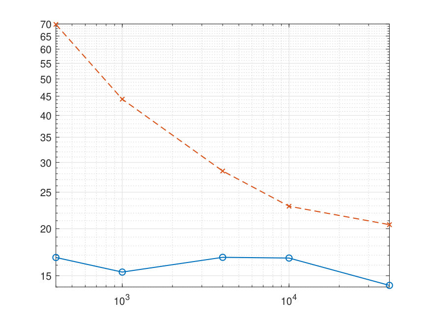 Figure 1
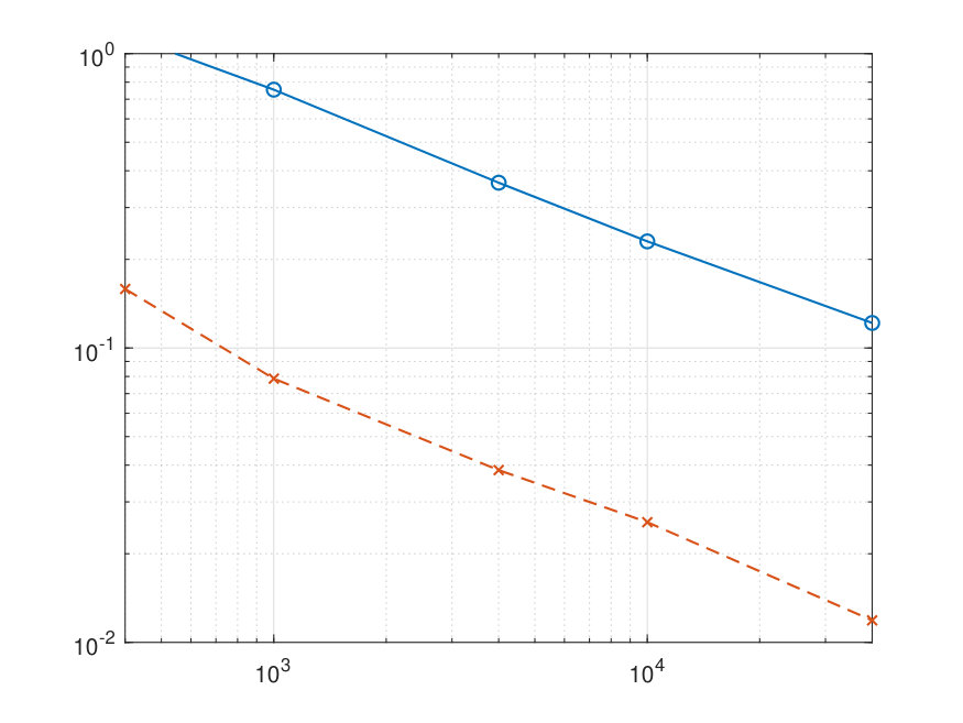 Figure 2
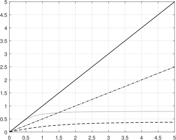 Figure 5
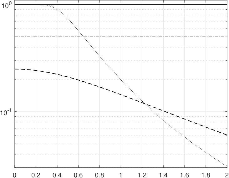 Figure 5
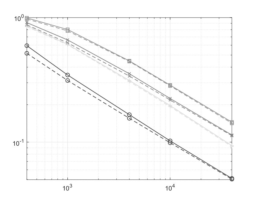 Figure 5
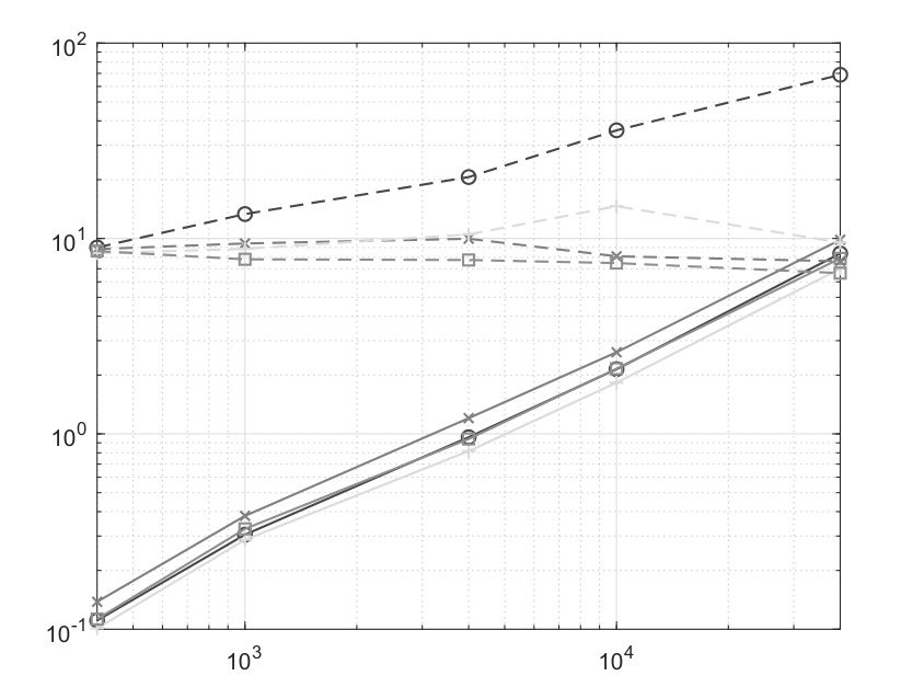 Figure 5
Peer Reviews
No public reviews on file for this paper yet. If you reviewed it on a platform where reviews are public (OpenReview, ICLR, NeurIPS, ICML), you can paste yours below so the community can read it here.
Videos
No videos yet. Explain this paper in a talk, walkthrough, or lecture? Add one.
Signal recovery by Stochastic Optimization
Anatoli Juditsky LJK, Université Grenoble Alpes, 700 Avenue Centrale 38401 Domaine Universitaire de Saint-Martin-d’Hères, France, [email protected]
Arkadi Nemirovski ISyE, Georgia Institute of Technology, Atlanta, Georgia 30332, USA, [email protected]
The first author was supported by the PGMO grant 2016-2032H. Research of the second author was supported by NSF grant CCF-1523768.
Abstract
We discuss an approach to signal recovery in Generalized Linear Models (GLM) in which the signal estimation problem is reduced to the problem of solving a stochastic monotone variational inequality (VI). The solution to the stochastic VI can be found in a computationally efficient way, and in the case when the VI is strongly monotone we derive finite-time upper bounds on the expected error converging to 0 at the rate as the number of observations grows. Our structural assumptions are essentially weaker than those necessary to ensure convexity of the optimization problem resulting from Maximum Likelihood estimation. In hindsight, the approach we promote can be traced back directly to the ideas behind the Rosenblatt’s perceptron algorithm.
1 Introduction
Statistical estimation problems constitute one of principal application domains of Stochastic Optimization. A typical setting is as follows (cf., e.g., [7] and references therein): we are given i.i.d. observations , , where , are, respectively, realizations of regressors (independent variables) and responses (labels). We assume that the observations can be described by a Generalized Linear Model (GLM) [13, 12], that is, the conditional, given, expectation of is , where is a known link function, and is the unknown “signal” — vector of model’s parameters. Our goal is to “fit the model,” that is, to recover from observations . The standard approach to fitting the model is to choose a loss function and to recover as an optimal solution to the optimization problem
[TABLE]
where is the distribution of the observation associated with “true signal ”, and is an a priori known signal set. In other words, in the just presented framework, the statistical estimation problem reduces to the stochastic optimization problem (1), which is to be solved approximately via available observation . This can be done either “in batch,” minimizing in the Sample Average Approximation (SAA)
[TABLE]
of the expectation in (1) (see, e.g. [19]), or applying iterative stochastic optimization algorithms of Stochastic Approximation (SA) type [16, 21].
Assuming that the conditional, given , distribution of induced by belongs to a known parameteric family , specifically, , the standard choice of the loss function is given by Maximum Likelihood: assuming that distributions have densities w.r.t. a reference measure , one uses
[TABLE]
For example, in the classical logistic regression , , , and , , is Bernoulli distribution, that is, label takes value 1 with probability and value 0 with the complementary probability, resulting in
[TABLE]
In this case, problem (1) becomes the optimization problem
[TABLE]
and its SAA becomes
[TABLE]
the optimal solution to the latter problem is the Maximum Likelihood (ML) estimate of . Assuming the signal set to be convex, both these problems turn out to be convex, implying the possibility to solve the SAA to global optimality in a computationally efficient fasion, same as utilizing nice convergence properties of SA.
More generally, when distributions of observations form a conditional exponential family [3, 9], negative log-likelihood has the form
[TABLE]
with convex cumulant function , and corresponding risk minimization problem (1) reads
[TABLE]
In this case, same as in the case of logistic regression, SAA or SA can be applied to compute Maximal Likelihood estimates of model parameter.
Note, however, that exponential family assumption is quite restrictive. On the other hand, beyond exponential families, the convexity of the optimization problem resulting from Maximum Likelihood selection of appears to be an exception rather than a rule. For example, consider the “nonlinear Least Squares” setting in which the label is obtained from by adding independent of the regressor zero mean Gaussian noise:
[TABLE]
In this case problem (1) and its SAA approximation for the ML selection of become
[TABLE]
where is the distribution of regressors (which we assume to be independent of the signal). When is nonlinear, both these problems usually are nonconvex and could be difficult to process numerically. Similarly, in the “non-exponential logistic regression,” where the “exponential sigmoid” is replaced with a general nondecreasing link function (e.g., probit or complementary link) the ML selection of the loss function typically makes (1) and its SAA approximation nonconvex.
The goal of what follows is to propose an alternative to model fitting via (1) with ML-based selection of the loss function approach to estimating the signal underlying observations in a GLM. In hindsight, the approach we put forward in this paper can be traced back to the ideas behind the Rosenblatt’s perceptron iterative algorithm [17, 4] and its batch version [10]. The structural assumptions to be imposed on the model are essentially weaker than those resulting in convex ML-based problems (1) and their SAA approximations.111For instance, in the “nonlinear least squares” with , same as in “non-exponential logistic regression,” all we need from to be continuously differentiable, with positive derivative, and from the signal set to be convex. Under these assumptions, instead of using the classical loss function approach [1, 8, 2, 5, 20], we reduce the estimation problem to another problem with convex structure — a strongly monotone variational inequality (VI) represented by a stochastic oracle. This VI may or may not be equivalent to a convex minimization problem. The first option definitely takes place when , when the VI is equivalent to analogous to (6) convex optimization problem; but even in this case the resulting problem typically is different from the ML version of (1). The solution to the VI can be found in a computationally efficient way and turns out to be a “good” estimate of the signal underlying observations, for which we derive finite-time upper bounds on the expected error, converging to 0 at the rate as .222We were unable to locate a reference to the proposed approach in the statistical literature, though it would be the most surprising if simple derivations which follow were not known.
2 Problem statement
Throughout the paper we consider the GLM model as posed in Introduction:
Our observation depends on unknown signal known to belong to a given convex compact set and is
[TABLE]
with , which are i.i.d. realizations of a random pair with the distribution such that
- •
the regressor is a random matrix with some independent of probability distribution ;
- •
the label is -dimensional random vector such that the conditional, given , distribution of induced by has the expectation :
[TABLE]
where is the conditional, given, distribution of stemming from the distribution of , and is a given mapping.
We are about to formulate assumptions on the parameters of a generalized linear model (namely, on , and the distributions , , of the pair ) required by the approach we are about to develop.
2.1 Preliminaries: monotone vector fields
A monotone vector field on is a single-valued everywhere defined mapping which possesses the monotonicity property
[TABLE]
We say that such a field is monotone with modulus on a closed convex set , if
[TABLE]
and say that is strongly monotone on if the modulus of monotonicity of on is positive. It is immediately seen that for a monotone vector field which is continuously differentiable on a closed convex set with a nonempty interior, the necessary and sufficient condition for being monotone with modulus on the set is
[TABLE]
Basic examples of monotone vector fields are:
- •
gradient fields of continuously differentiable convex functions of variables or, more generally, the vector fields stemming from continuously differentiable functions which are convex in and concave in ;
- •
“diagonal” vector fields with monotonically nondecreasing univariate components . If, in addition, are continuously differentiable with positive derivatives, then the associated field is strongly monotone on every compact convex subset of , the monotonicity modulus depending on the subset.
Monotone vector fields on admit simple calculus which includes, in particular, the following two rules:
- I.
[affine substitution of argument]: If is monotone vector field on and is an matrix, the vector field
[TABLE]
is monotone on ; if, in addition, is monotone with modulus on a closed convex set and is closed, convex, and such that whenever , is monotone with modulus on , where is the minimal singular value of .
- II.
[summation]: If is a Polish space, is a Borel vector-valued function which is monotone in for every and is a Borel probability measure on such that the vector field
[TABLE]
is well defined for all , then is monotone. If, in addition, is a closed convex set in and is monotone on with Borel in modulus for every , then is monotone on with modulus .
2.2 Assumptions
In what follows, we make the following assumptions on the ingredients of the estimation problem set in Introduction:
- •
A.1. The vector field is continuous and monotone, and the vector field
[TABLE]
is well defined (and therefore is monotone along with by I, II);
- •
A.2. The signal set is a nonempty convex compact set, and the vector field is monotone with positive modulus on ;
- •
A.3. For properly selected and every it holds
[TABLE]
A simple sufficient condition for the validity of Assumptions A.1-3 with properly selected and is as follows:
- •
The distribution of has finite moments of all orders, and ;
- •
is continuously differentiable, and for all and all . Besides this, is of polynomial growth: for some constants and and all one has .
Verification of sufficiency is straightforward.
3 Construction and Main result
The principal observation underlying the construction we are about to present is as follows:
Proposition 3.1
Assuming that Assumptions A.1-3 hold, let us associate with the pair the vector field
[TABLE]
Then for every we have
[TABLE]
Proof is immediate. Indeed, let . Then
[TABLE]
(we have used (9) and the definition of ), whence,
[TABLE]
as stated in (13.). Besides this, for , denoting by the conditional, given, distribution of induced by the distribution of , and taking into account that the marginal distribution of induced by is , we have
[TABLE]
This combines with the relation given by A.3 due to to imply (13.) and (13.).
3.1 Main result
Recall that our goal is to recover the signal underlying observations (8). Under assumptions A.1-3, is a root of the monotone vector field
[TABLE]
we know that this root belongs to , and is unique because is strongly monotone on along with . Now, finding a root, known to belong to a given convex compact set , of a strongly monotone on this set vector field is known to be a computationally tractable problem, provided we have access to an “oracle” which, given on input a point , returns the value of the field at the point. The latter is not exactly the case in the situation we are interested in: the field is the expectation of a random field:
[TABLE]
and we do not know a priori what is the distribution over which the expectation is taken. However, we can sample from this distribution – the samples are exactly the observations (8), and we can use these samples to approximate somehow and use this approximation to approximate the signal . Two standard implementations of this idea are Sample Average Approximation (SAA) and Stochastic Approximation (SA). We are about to consider these two techniques as applied to the situation we are in.
3.1.1 Estimation by Sample Average Approximation
The idea underlying SAA is quite transparent: given observations (8), let us approximate the field of interest with its empirical counterpart
[TABLE]
By the Law of Large Numbers, as , the empirical field converges to the field of interest , so that under mild regularity assumptions, when is large, , with overwhelming probability, will be uniformly on close to . Due to strong monotonicity of , this would imply that a set of “near-zeros” of on will be close to the zero of , which is nothing but the signal we want to recover. The only question is how we can consistently define a “near-zero” of on .333Note that we in general cannot define a “near-zero” of on as a root of on this set – while does have a root belonging to , nobody told us that the same holds true for . A convenient in our context notion of a “near-zero” is provided by the concept of a weak solution to a variational inequality (VI) with monotone operator, defined as follows (we restrict the general definition to the situation of interest):
Let be a nonempty convex compact set, and be a monotone (i.e., for all ) vector field. A vector is called a weak solution to the variational inequality (VI) associated with when
[TABLE]
Let be a nonempty convex compact set and be monotone on . It is well known that
- •
The VI associated with (let us denote it ) always has a weak solution. It is clear that if is a root of , then is a weak solution to .444Indeed, when and , monotonicity of implies that for all , that is, is a weak solution to the VI.
- •
When is continuous on , every weak solution to is also a strong solution, meaning that
[TABLE]
Indeed, (15) clearly holds true when . Assuming and setting , , we have (since is a weak solution), whence (since is a positive multiple of ). Passing to limit as and invoking the continuity of , we get , as claimed.
- •
When is the gradient field of a continuously differentiable convex function on (such a field indeed is monotone), weak (or, which in the case of continuous is the same, strong) solutions to are exactly the minimizers of the function on .
Note also that a strong solution to with monotone always is a weak one: if satisfies for all , then for all , since by monotonicity .
In the sequel, we heavily exploit the following simple and well known fact:
Lemma 3.1
Let be a convex compact set, and be a monotone vector field on with monotonicity modulus , i.e.
[TABLE]
Further, let be a weak solution to . Then the weak solution to is unique. Besides this,
[TABLE]
Proof: Under the premise of the lemma, let and let be a weak solution to (recall that it does exist). Setting , for we have
[TABLE]
where the first is due to strong monotonicity of , and the second is due to the fact that is proportional, with positive coefficient, to , and the latter quantity is nonnegative since is a weak solution to the VI in question. We end up with ; passing to limit as , we arrive at (16). To prove uniqueness of a weak solution, assume that aside of the weak solution there exists a weak solution distinct form , and let us set . Since both and are weak solutions, both the quantities and should be nonnegative, and because the sum of these quantities is 0, both of them are zero. Thus, when applying (16) to , we get , whence as well.
Now, let us return to the estimation problem under consideration. Assume that Assumptions A.1-3 hold, so vector fields defined in (12), and therefore vector field are continuous and monotone. When using the SAA, we compute a weak solution to and treat it as the SAA estimate of signal underlying observations (8). Since the vector field is monotone with efficiently computable values, provided that so is , computing (a high accuracy approximation to) a weak solution to is a computationally tractable problem (see, e.g., [14]). Moreover, utilizing the techniques from [6, 15, 20, 18], under mild additional to A.1-3 regularity assumptions one can get non-asymptotical upper bound on, say, the expected -error of the SAA estimate as a function of the sample size and find out the rate at which this bound converges to 0 as ; this analysis, however, goes beyond our scope.
Let us look at the SAA estimate in the logistic regression model. In this case we have , and
[TABLE]
In other words, is the gradient field of the minus empirical log-likelihood , see (5). As a result, in the case in question weak solutions to are exactly the optimal solutions to (5), that is, for the logistic regression the SAA estimate is nothing but the Maximum Likelihood estimate .555This phenomenon is specific for the logistic regression model. The fact that the SAA and the ML estimates in this case are the same is due to the fact that the logistic sigmoid “happens” to satisfy the identity . When replacing the exponential sigmoid with with differentiable monotonically nondecreasing positive , the SAA estimate becomes the weak solution to with
On the other hand, the gradient field of the minus log-likelihood ) which we should minimize when computing the ML estimate is
When and is not an exponent, and are “essentially different,” so that the SAA estimate typically will differ from the ML one. On the other hand, in the “nonlinear least squares” example described in the introduction with (for the sake of simplicity, scalar) monotone the vector field is given by
[TABLE]
which is “essentially different” (provided that is nonlinear) from the gradient field
[TABLE]
of the negative log-likelihood appearing in (7). As a result, in this case the ML estimate (7) is, in general, different from the SAA estimate (and, in contrast to the ML, the SAA estimate is easy to compute).
3.1.2 Stochastic Approximation estimate
The Stochastic Approximation (SA) estimate stems from a simple algorithm – Subgradient Descent – for solving variational inequality . Were the values of the vector field available, one could approximate a root of this VI using the recurrence
[TABLE]
where
- •
is the metric projection of onto :
[TABLE]
- •
are given stepsizes;
- •
the initial point is an arbitrary point of .
It is well known that under Assumptions A.1-3 this recurrence with properly selected stepsizes and started at a point from allows to approximate the root of (in fact, the unique weak solution to ) to a whatever high accuracy, provided is large enough. However, we are in the situation when the actual values of are not available; the standard way to cope with this difficulty is to replace in the above recurrence the “unobservable” values of with their unbiased random estimates . This modification gives rise to Stochastic Approximation (coming back to [11]) – the recurrence
[TABLE]
where is a once for ever chosen point from , and are deterministic.
Convergence analysis.
The following result is perfectly well known; to make the paper self-contained, we present its (completely standard) proof in Appendix.
Proposition 3.2
Under Assumptions A.1-3 and with the stepsizes
[TABLE]
for every signal the sequence of estimates given by the SA recurrence (17) and defined in (8) for every obeys the error bound
[TABLE]
* being the distribution of stemming from signal .*
3.2 Numerical illustration
To illustrate the above developments, we present here results of some numerical experiments. Our deliberately simplistic setup is as follows:
- •
;
- •
the distribution of is ;
- •
is the monotone vector field on given by one of the following four options:
- A.
;
- B.
;
- C.
;
- D.
.
- •
conditional, given , distribution of induced by is
- –
Bernoulli distribution with probability of outcome 1 in the case of A (i.e., A corresponds to the logistic model),
- –
Gaussian distribution in cases B – D.
Note that in the considered example one can easily compute the field . Indeed, we have :
[TABLE]
and due to the independence of and ,
[TABLE]
and is proportional to with proportionality coefficient
[TABLE]
In Figure 1 we present the plots of the function for the situations A – D, same as the dependencies of the moduli of strong convexity of the corresponding mappings in a centered at the origin -ball of radius on .
The dimension in all experiments was set to 100, and the number of observations was , 1e3, 4e3, 1e4, and 4e4. For each combination of parameters we ran 10 simulations for signals underlying observations (8) drawn randomly from the uniform distribution on the unit sphere (the boundary of ).
In each experiment, we computed the SAA and the SA estimates (note that in the cases A and B the SAA estimate is the Maximum Likelihood estimate as well). The SA stepsizes were selected according to (18) with “empirically selected” . 666We could get (lower bounds on) the modules of strong monotonicity of the vectors fields we are interested in analytically, but this would be boring and conservative. Namely, given observations , , see (8), we used them to build the SA estimate in two stages:
— at tuning stage, we generate a random “training signal” and then generate labels as if were the actual signal. For instance, in the case of A, is assigned value 1 with probability and value 0 with complementary probability. After “training signal” and associated labels are generated, we run on the resulting artificial observations SA with different values of , compute the accuracy of the resulting estimates, and select the value of resulting in the best recovery;
— at execution stage, we run SA on the actual data with stepsizes (18) specified by found at the tuning stage.
The results of some numerical experiments are presented in Figure 2.
Note that the cpu time for SA includes both tuning and execution stages. The conclusion from these experiments is that as far as estimation quality is concerned, the SAA estimate marginally outperforms the SA, while being significantly more time consuming. Note also that the observed in our experiments dependence of recovery errors on is consistent with the convergence rate established by Proposition 3.2.
4 “Single-observation” case
Let us look at the special case of the estimation problem where the sequence of regressors in (8) is deterministic. At the first glance, this situation goes beyond our setup, where the regressors should be i.i.d. drawn from some distribution . We can, however, circumvent this “contradiction” by saying that we are now in the single-observation case with the regressor being the matrix and being a degenerate distribution supported at a singleton. Specifically, consider the case where our observation is
[TABLE]
( are given positive integers), and the distribution of observation stemming from a signal is as follows:
- •
is a given independent of deterministic matrix;
- •
is random, and the distribution of induced by is with mean , where is a given mapping.
As an instructive example connecting our current setup with the previous one, consider the case where with deterministic “individual regressors” , with random “individual labels” conditionally independent, given , across , and such that the induced by expectations of are for some . We set . The resulting “single observation” model is a natural analogy of the -observation model considered so far, the only difference being that the individual regressors now form a fixed deterministic sequence rather than being a sample of some random matrix.
Same as everywhere in this paper, our goal is to use observation (20) to recover the (unknown) signal underlying, as explained above, the distribution of the observation. Formally, we are now in the case of our previous recovery problem where is supported on a singleton and can use the constructions developed so far. Specifically,
- •
The vector field associated with our problem (it used to be ) is
[TABLE]
and the vector field being the signal underlying observation (20), is
[TABLE]
(cf. (14)). Same as before, the signal to recover is a zero of the latter field. Note that now the vector field is observable, and the vector field still is the expectation, over , of an observable vector field:
[TABLE]
cf. Lemma 3.1.
- •
Assumptions A.1-2 now read
A.1′ The vector field is continuous and monotone, so that is continuous and monotone as well,
A.2′ is a nonempty compact convex set, and is strongly monotone, with modulus , on .
A simple sufficient condition for the validity of the above monotonicity assumptions is positive definiteness of the matrix plus strong monotonicity of on every bounded set.
- •
For our present purposes, it is convenient to reformulate assumption A.3 in the following equivalent form:
A.3′ For properly selected and every it holds
[TABLE]
In the present setting, the SAA estimate is the unique weak solution to , and we can easily quantify the quality of this estimate:
Proposition 4.1
In the situation in question, let Assumptions A.1′-3′ hold. Then for every and every realization of induced by observation (20) one has
[TABLE]
whence also
[TABLE]
Proof. Let be the signal underlying observation (20), and be the associated vector field . We have
[TABLE]
For fixed, is the weak, and therefore the strong (since is continuous) solution to , implying, due to , that
[TABLE]
whence
[TABLE]
Besides this, , whence , and we arrive at
[TABLE]
whence also
[TABLE]
(recall that , along with , is strongly monotone with modulus on and ). Applying the Cauchy inequality, we arrive at (21).
Example. Consider the case where , is strongly monotone, with modulus , on the entire , and in (20) is drawn from a “Gaussian ensemble” – the columns of the matrix are independent -random vectors. Assume also that the observation noise is Gaussian:
[TABLE]
It is well known that as , the minimal singular value of the matrix is at least with overwhelming probability, implying that when , the typical modulus of strong monotonicity of is . Furthermore, in our situation, as , the Frobenius norm of with overwhelming probability is at most . In other words, when is large, a “typical” recovery problem from the just described ensemble satisfies the premise of Proposition 4.1 with and . As a result, (22) reads
[TABLE]
It is well known that in the standard case of linear regression, where , the resulting bound is near-optimal, provided is large enough.
Numerical illustration: in the situation described in the example above, we set , and use
[TABLE]
The set is the unit ball . In a particular experiment, is chosen at random from the Gaussian ensemble as described above, and signal underlying observation (20) is drawn at random; the observation noise is . We ran 10 simulations for each combination of the samples size and noise variance ; the results are presented in Figure 3.
Appendix A Proof of Proposition 3.2
We start by observing that are deterministic functions of the initial fragments of our sequence of observations : . Let us set
[TABLE]
where is the signal underlying observations (8). Note that, as it is well known, the metric projection onto a closed convex set is contracting:
[TABLE]
Consequently, for it holds
[TABLE]
Taking expectations w.r.t. of both sides of the resulting inequality and keeping in mind relations (13) along with the fact that , we get
[TABLE]
Recalling that we are in the case where is strongly monotone on with modulus , is the weak solution , and takes values in , invoking (16), the expectation in (23) is at least , and we arrive at the relation
[TABLE]
We put
[TABLE]
note that are exactly the stepsizes (18). Let us verify by induction in that for it holds
[TABLE]
Base . Let stand for the -diameter of , and be such that . By (13) we have for all , and by strong monotonicity of on we have
[TABLE]
By Cauchy inequality, the left hand side in the concluding is at most , and we get
[TABLE]
whence . On the other hand, due to the origin of we have . Thus, holds true.
Inductive step . Now assume that holds true for some , , and let us prove that holds true as well. Observe that , so that
[TABLE]
so that hods true. Induction is complete. It remains to note that by definition of we have .
The reference list from the paper itself. Each links out to its DOI / PubMed record.
- 1[1] M. Aiserman, E. M. Braverman, and L. Rozonoer. Theoretical foundations of the potential function method in pattern recognition. Avtomat. i Telemeh , 25:917–936, 1964.
- 2[2] M. Aizerman, E. Braverman, and L. Rozonoer. Method of potential functions in the theory of learning machines . Nauka, Moscow, 1970.
- 3[3] O. Barndorff-Nielsen. Information and exponential families in statistical theory. 1978.
- 4[4] H.-D. Block. The perceptron: A model for brain functioning. i. Reviews of Modern Physics , 34(1):123, 1962.
- 5[5] O. Bousquet, S. Boucheron, and G. Lugosi. Introduction to statistical learning theory. In Advanced lectures on machine learning , pages 169–207. Springer, 2004.
- 6[6] O. Bousquet and A. Elisseeff. Stability and generalization. Journal of machine learning research , 2(Mar):499–526, 2002.
- 7[7] L. Devroye, L. Györfi, and G. Lugosi. A probabilistic theory of pattern recognition , volume 31. Springer Science & Business Media, 2013.
- 8[8] I. Devyaterikov, A. Propoi, and Y. Z. Tsypkin. Iterative learning algorithms for pattern recognition. Automation and Remote Control , 28:122–132, 1967.