Data-Enabled Predictive Control for Grid-Connected Power Converters
Linbin Huang, Jeremy Coulson, John Lygeros, Florian Dorfler

TL;DR
This paper introduces a data-driven control approach for grid-connected power converters, combining DeePC and ARMA-based MPC to improve stability and performance without relying on explicit system models.
Contribution
It presents a novel combination of DeePC and ARMA-based MPC methods, addressing scalability issues and demonstrating effectiveness in stabilizing power converters.
Findings
DeePC eliminates undesired oscillations in power converters.
ARMA-based MPC improves scalability for high-order systems.
The combined approach stabilizes a voltage source converter in a power system.
Abstract
We apply a novel data-enabled predictive control (DeePC) algorithm in grid-connected power converters to perform safe and optimal control. Rather than a model, the DeePC algorithm solely needs input/output data measured from the unknown system to predict future trajectories. We show that the DeePC can eliminate undesired oscillations in a grid-connected power converter and stabilize an unstable system. However, the DeePC algorithm may suffer from poor scalability when applied in high-order systems. To this end, we present a finite-horizon output-based model predictive control (MPC) for grid-connected power converters, which uses an N-step auto-regressive-moving-average (ARMA) model for system representation. The ARMA model is identified via an N-step prediction error method (PEM) in a recursive way. We investigate the connection between the DeePC and the concatenated PEM-MPC method, and…
Click any figure to enlarge with its caption.
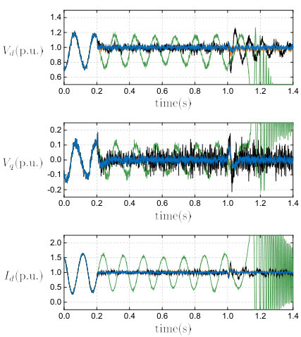 Figure 1
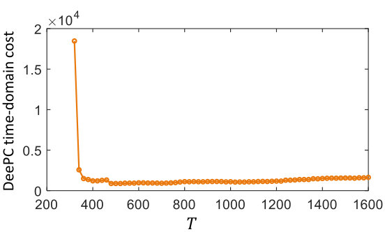 Figure 2
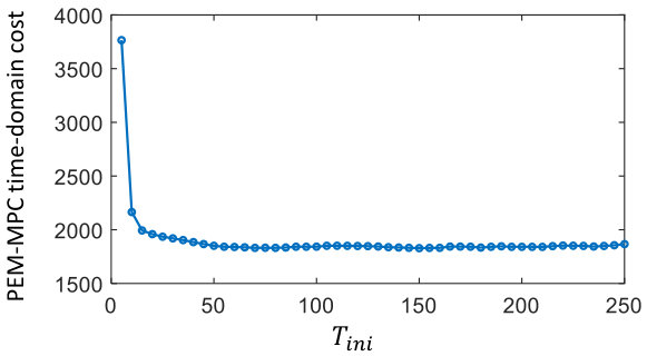 Figure 3
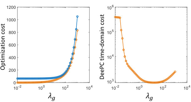 Figure 4
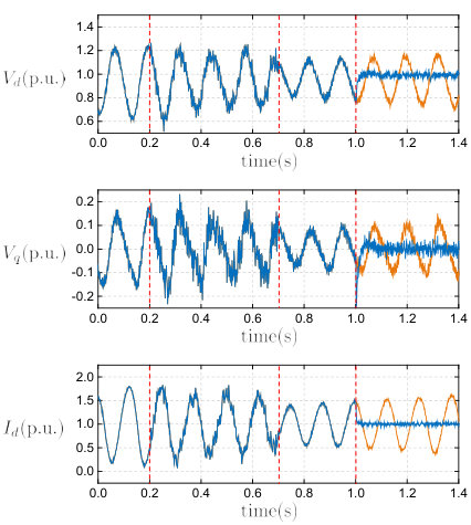 Figure 5
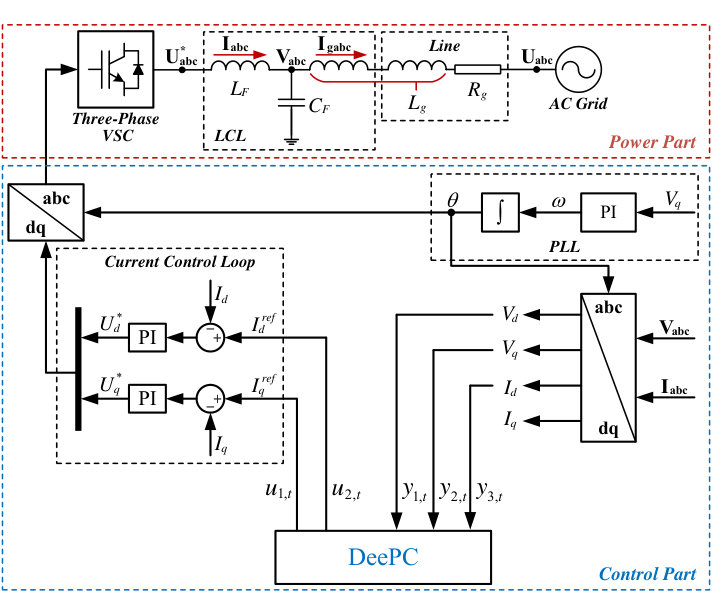 Figure 6
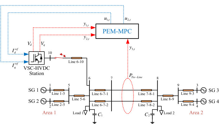 Figure 7
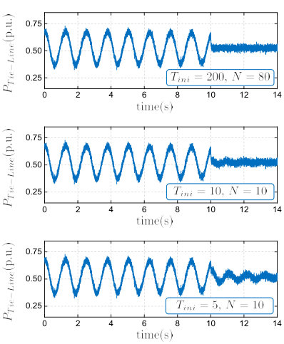 Figure 8
| Base Values for Per-unit Calculation | |
| Voltage base value: | Power base value: |
| Frequency base value: | |
| Parameters of the Power Part (per-unit values) | |
| Converter-side inductor: | LCL capacitor: |
| Grid-side inductor: | Grid-side resistor: |
| Parameters of the Control Part | |
| PI gains of the PLL: | |
| PI gains of the current control loop: | |
| Control frequency for the digital signal processor: | |
| Parameters of the DeePC | |
| Length of the initial trajectories: | |
| Length of the prediction horizon: | |
| Length of the data to construct the Hankel matrix: | |
| Sampling frequency for the DeePC: | |
| Control cost: | Output cost: |
| Reference vector : | |
| Constraint set : | |
| Constraint set : | |
| Regularization parameter: | |
Peer Reviews
No public reviews on file for this paper yet. If you reviewed it on a platform where reviews are public (OpenReview, ICLR, NeurIPS, ICML), you can paste yours below so the community can read it here.
Videos
No videos yet. Explain this paper in a talk, walkthrough, or lecture? Add one.
Data-Enabled Predictive Control for Grid-Connected Power Converters
Linbin Huang, Jeremy Coulson, John Lygeros and Florian Dörfler L. Huang is with the College of Electrical Engineering at Zhejiang University, Hangzhou, China, and the Department of Information Technology and Electrical Engineering at ETH Zürich, Switzerland. (Email: [email protected])J. Coulson, J. Lygeros and F. Dörfler are with the Department of Information Technology and Electrical Engineering at ETH Zürich, Switzerland. (Emails: [email protected], [email protected], [email protected])This research was supported by ETH Zürich Funds.
Abstract
We apply a novel data-enabled predictive control (DeePC) algorithm in grid-connected power converters to perform safe and optimal control. Rather than a model, the DeePC algorithm solely needs input/output data measured from the unknown system to predict future trajectories. We show that the DeePC can eliminate undesired oscillations in a grid-connected power converter and stabilize an unstable system. However, the DeePC algorithm may suffer from poor scalability when applied in high-order systems. To this end, we present a finite-horizon output-based model predictive control (MPC) for grid-connected power converters, which uses an N-step auto-regressive-moving-average (ARMA) model for system representation. The ARMA model is identified via an N-step prediction error method (PEM) in a recursive way. We investigate the connection between the DeePC and the concatenated PEM-MPC method, and then analytically and numerically compare their closed-loop performance. Moreover, the PEM-MPC is applied in a voltage source converter based HVDC station which is connected to a two-area power system so as to eliminate low-frequency oscillations. All of our results are illustrated with high-fidelity, nonlinear, and noisy simulations.
I Introduction
The penetration of power-electronic devices in modern power systems is ever-increasing due to the development of renewable energy, microgrids, high-voltage direct-current (HVDC) transmission systems, etc. [1, 2]. This tendency is posing great challenges to power system operations because the dynamics of power converters are substantially different from synchronous generators (SGs). For example, SGs have large rotational rotors which physically determine the output frequencies, while power converters consist of static semiconductor apparatus and have high controllability.
Conventionally, the control structure of power converters is designed according to engineering experience and the corresponding control gain tuning is based on iterative trial-and-error methods. Also, lots of effort has been put into the modeling of power converters, which provides insights into the system dynamics and criteria for control gain tuning [3, 4, 5]. However, these approaches heavily rely on rich engineering experience and lack systematicness. In addition, the control structure generally assumes a stiff power grid and may present poor robustness against variable grid conditions. For example, the most widely-used control structure, which consists of a phase-locked loop (PLL) and a current control loop, can become unstable when the power converter is connected to a weak grid with high grid impedance (or equivalently, low short-circuit ratio) [6, 7, 8].
Even though offline design and analysis (based on a nominal model) can be conducted to determine an optimal control parameter set, optimal performance can rarely be achieved during online operation because (i) the real parameters of the power converter (e.g., capacitance and inductances of the LCL filter) are hard to obtain due to different operation conditions and manufacturing inaccuracy; (ii) sometimes the underlying algorithms for the converter are designed by another manufacturer and are not obtainable, i.e., some part of the converter system is unknown; (iii) the power grid is generally an unknown system from power converter side which significantly affects the dynamic performance; and (iv) the offline design generally employs a constant power grid model (which in most cases is assumed to be an infinite bus) for the power converter, yet the real power grid is variable.
Normally, these problems are handled using robust or adaptive methods [9, 8]. However, these methods are still model-based, result in complex controllers, and suffer from scalability problems for large and uncertain (or even partially unknown) models – especially, in grid-connected applications. Inspired by recent advances in machine learning and artificial intelligence, recent control approaches entirely circumvent such model-based solutions in favor of data-driven approaches [10, 11, 12].
In this paper, we use a novel Data-enabled Predictive Control (DeePC) algorithm to compute optimal and safe control policies for grid-connected power converters, which uses real-time feedback to drive the unknown system along a desired (i.e., optimal and constrained) trajectory [13]. The DeePC algorithm presented in [13] relies on behavioural system approach [14, 15, 16, 17]. Instead of using a parametric model for system representation (e.g., state space matrices obtained from system identification), the approach in [14, 15, 16, 17] describes the input/output behaviour of the system through the subspace of the signal space in which trajectories live. This signal space of trajectories is spanned by the columns of a data Hankel matrix which results in a non-parametric and data-centric perspective on dynamical control systems.
The DeePC approach presented here relies on input/output data samples from the converter-internal signals and terminal signals towards the power grid (whose model is unknown from the perspective of the converter’s controller), and successfully eliminates undesired oscillations by solving the optimal regulation problem in a receding horizon manner – with the input/output constraints incorporated and in absence of any system model. However, when applied in large-scale systems, e.g., in the case of power transmision oscillation damping [18, 19], the optimal regulation problem in DeePC may suffer from poor scalability due to its high dimension.
To this end, we use a finite-horizon output-based model predictive control (MPC) for grid-connected power converters, wherein the unknown system is represented by an -step auto-regressive-moving-average (ARMA) model and identified via least-square -step prediction error method (PEM). The PEM can be solved in a recursive way which enables an iterative calculation and possible online implementation. We will show that this concatenated PEM-MPC method is scalable for large-scale unknown systems, and analytically discuss how it is related to DeePC. Namely, DeePC provably outperforms the PEM-MPC method in terms of the cost in the optimal regulation problem (see Lemma III.2) although this performance gap can be made smaller by appropriate regularizations of the optimal control and system identification problems. We propose to use the PEM-MPC in a grid-connected voltage source converter (VSC) based HVDC station to attenuate the power system oscillations which are caused by the interactions among multiple synchronous generators [20]. All of our results are illustrated with high-fidelity nonlinear simulations.
The remainder of this paper is organized as follows: in Section II we provide an overview for the DeePC approach and apply it to a grid-connected power converter. Section III presents the concatenated PEM-MPC and we discuss how it is related to DeePC. In Section IV we apply the PEM-MPC in a two-area power system which contains one VSC-HVDC station. We conclude the paper in Section V.
II Data-Enabled Predictive Control
II-A Preliminaries and Notation
For an unknown discrete-time LTI system that has inputs and outputs, we denote by the input of the system at time and the output at time , where is the discrete-time axis. The input vector of the system is denoted by , and the output vector is denoted by , where . Let and be the input and output trajectories, respectively, whose dimensions can be inferred from the context.
Let and . The trajectory is persistently exciting of order L if the Hankel matrix
[TABLE]
is of full row rank, i.e., the signal is sufficiently long and sufficiently rich.
Consider the following -order discrete-time LTI system (minimal representation):
[TABLE]
where , , , , and is the state of the system at time .
The lag of the system in (2) is defined by the smallest integer so that the observability matrix
[TABLE]
has rank .
Let such that . Consider an input trajectory and an output trajectory (both are of length , i.e., and ) measured from the -order unknown system (2) such that is persistently exciting of order . Here we use the superscript d to indicate that these two trajectories are data sets measured from the unknown system. We use and to construct the Hankel matrices and , which are further partitioned into two parts as
[TABLE]
where , , and .
According to the behavioral system theory [15], is a trajectory of (2) if and only if there exist such that
[TABLE]
The trajectory can be thought of as an initial condition for the trajectory and as a future trajectory departing from this initial condition. If , the future output trajectory is uniquely determined through (4) for every given input trajectory .
II-B Review of DeePC
Instead of learning a parametric system representation through system identification, the DeePC attempts to learn the system’s behaviour and computes optimal control inputs using past data measured from the unknown system. Moreover, input/output constraints can be conveniently incorporated to ensure safety, described as follows.
After using the input/output trajectory ( and ) to construct the Hankel matrices in (3), DeePC solves the following optimization problem at every sampling time to get the optimal future control inputs
[TABLE]
where and are the input and output constraint sets, is the control cost matrix (positive definite), is the output cost matrix (positive semidefinite), is the regularization parameter, is the reference vector for the output signals, is the prediction horizon, and consists of the most recent input/output trajectory of (2). The norm of the vector denotes the quadratic form , and the norm denotes .
We note that a two-norm penalty on is included in the cost function as a regularization term to avoid overfitting. In fact, in the case when stochastic disturbances affect the output measurements, a two-norm regularization on coincides with two-norm robustness with respect to the noise affecting the output measurements [21]. The DeePC involves solving the optimization problem (DeePC) in a receding horizon manner [13], that is, after calculating the optimal control input sequence , we apply to the system for some time steps, update to the most recent input/output measurements and then set to for the DeePC algorithm.
II-C Application to a Grid-Connected Power Converter
Fig.1 shows the one-line diagram of a three-phase power converter which is connected to an ac power grid via an LCL. The system is nonlinear (the nonlinearity comes from the coordinate transformation), and the order of the system is . Here, the ac power grid is modeled as an infinite bus with fixed voltage magnitude and frequency . The base values for per-unit calculation and the system parameters are given in Table I, wherein the symbol denotes the column vector with all the entries being , and denotes the column vector with all the entries being [math], is the identity matrix whose dimension can be inferred from the text, and the Kronecker product of and is denoted by . The control part of the converter consists of a synchronous reference frame PLL, a current control loop and coordinate transformation blocks [4, 22].
The current control loop contains two proportional-integral (PI) regulators to make the converter-side d-axis and q-axis current components (i.e., and as shown in Fig.1) track their references and , which enables fast current limiting under faults and harmonic suppression of the converter-side current.
The PLL is used for grid-synchronization. The input of the PLL is the q-axis voltage component (i.e., ) of the LCL’s capacitor, and the output is the angle reference for coordinate transformation. The -axis voltage component is controlled to be zero in steady state via the PI regulator in the PLL, and therefore the voltage vector is aligned with the d-axis, that is, the d-axis voltage component (i.e., ) is the magnitude of the capacitor’s voltage vector in steady state.
When the converter is connected to a strong grid that features low grid-side impedance, it will present anticipated dynamic performance. However, one significant challenge for the converter’s operation is that generally the converter does not have any information about the properties of the ac power grid. If the converter is connected to a weak grid that has high grid-side impedance, e.g., as used in this section, the PLL will have significant interaction with the current control loop as well as the grid impedance, which may result in instabilities of the system [23, 8]. This kind of small-signal instability features the oscillations of the PLL’s output and current/voltage signals, which should be eliminated to ensure the safe operation of the power grid.
In this section, we use the DeePC to perform optimal control for the converter that is connected to a weak ac grid, which can attenuate the oscillations in the converter and stabilize the system by penalizing the tracking errors in the cost function. The power converter together with the power grid is a black-box system from the view of the DeePC. The DeePC provides control inputs to this black-box system and measures its input/output trajectories with sampling frequency (i.e., sampling time ).
We choose and to be the control inputs considering that the current control loop has high response speed and allows fast current limiting. The measured outputs from the black-box system are , and , which will be controlled to track their references via the DeePC. These output signals contain measurement noise (white noise with noise power: ). We note that , which corresponds to the reactive current, is not chosen as the measured output for the DeePC because is uniquely determined by the power flow constraint when , and equal their reference values in steady state. Since the DeePC has no information about the black-box system, is chosen to be sufficiently large () to meet .
Fig.2 plots the time-domain responses of the power converter. When the DeePC is activated at , the voltage/current oscillations are effectively eliminated. By comparison, the system is unstable without the DeePC (where and are respectively set as and [math]), and there are voltage/current oscillations whose magnitudes are amplified over time. These simulation results verify the effectiveness of using DeePC to perform optimal predictive control for a grid-connected power converter with unknown grid conditions (e.g., grid-side impedance and grid properties) and unknown converter model and inner controls.
III From DeePC to MPC
III-A Scalability of DeePC
The DeePC approach provides a safe and optimal solution to the regulation problem by solely using the measured data from the unknown system, and thus allows to stabilize an unknown and unstable system, as illustrated in the previous case study. However, when applied in high-order systems, the DeePC may suffer from poor scalability because the dimension of the decision variable (which is ) depends on the length of data to construct the Hankel matrix. In other words, the optimization problem in (DeePC) is of high dimension when choosing a long sequence of data to possibly eliminate the impacts of measurement noise.
To remove from the constraint and ensure the scalability of the optimization problem in (DeePC), we consider a subsequent system identification and model predictive control whose decision variables are and .
III-B Model Predictive Control
In what follows, we consider the following finite-horizon output-based MPC problem
[TABLE]
where the decision variables and are the control inputs and measurement outputs over the prediction horizon, and is the -step transition matrix predicting how future outputs of the system are determined by the initial input/output data and the future inputs. Note that the optimization problem (MPC) is solved in a receding horizon manner resulting in an online feedback control.
Since the decision variable in (DeePC) does not appear in (MPC), solving (MPC) has much less computational burden than solving (DeePC), especially when the Hankel matrix has high column number (i.e., has high dimension). On the other hand, (MPC) depends on an explicit predictive model given by the transition matrix in the equality constraint.
III-C Prediction Error System Identification
Observe that the predictive model in (MPC) is an -step ARMA model for the discrete-time LTI system mapping past inputs and outputs as well as future inputs to future outputs . In particular, for the () element of , we have
[TABLE]
where is the row of and .
Given past measurements of and , the transition matrix can be computed offline through system identification. In the absence of measurement noise, can be computed exactly with linearly independent measurements of and associated . However, measurement noise will significantly affect the accuracy of this approach. A standard solution to remedy this problem and to eliminate the effects of the noise is to use a larger data set and apply a least-square -step PEM minimizing
[TABLE]
where is the number of measured trajectories, and and belong to the trajectory. Indeed, the subsequent combination of PEM and MPC is a standard approach to model-based control that has proved itself in many applications throughout academia and industry [24, 25].
As an alternative to the batch optimization approach (PEM) combining all the measured trajectories to solve for in one step, can be obtained by adopting the recursive least-square algorithm [26]
[TABLE]
where is the least-square solution for after combining the previous trajectories, and is updated to using the data (i.e., and ) in the trajectory. The matrices and are two intermediate variables updated through the trajectory in the recursive algorithm.
The recursive algorithm (6) is not only more scalable for large data sets, but it could possibly also be applied online to adapt the model used in (MPC) to a variable environment. Moreover, the size of is solely related to and and independent of the size of the data set, which leads to a smaller optimization problem size than (DeePC) when applied to high-order systems, considering that the dimension of the decision variable in (DeePC) depends on the length of the data to construct the Hankel matrix.
III-D Relation of DeePC, MPC, and PEM
In the following, we will relate the subsequent system identification through (PEM) and model-based control through (MPC) to the data-driven (DeePC) strategy. In a first step, observe that the least-square solution for (PEM) can be expressed in closed form as
[TABLE]
where the Moore-Penrose pseudoinverse of the matrix is denoted by .
The transition matrix can then be obtained as
[TABLE]
Since every column in the constructed Hankel matrix (3) is one trajectory measured from the unknown system, can also be calculated by using the Hankel matrix (3) by
[TABLE]
By combining (9) with and one obtains
[TABLE]
which equals the solution of the optimization problem
[TABLE]
Observe that the optimization problem (LN) seeks the least-norm solution to the equality constraint. Thus, we refer to it as the least-norm (LN) problem. As derived above, for Hankel matrix data, the solution of (LN) is related to the solution of the least-squares (PEM) problem by . It can also be derived using subspace identification methods [17]. We summarize this observation below.
Lemma III.1** (PEM and LN)**
Consider the least-norm problem (LN) with Hankel matrix . Consider the least-square -step prediction error method optimization problem (PEM), and assume that its data and is arranged into the Hankel matrix . Then the solution of (PEM) and the solution of (LN) are related by the equation .
Observe that if the (LN) solution is used as predictive model (equality constraint) of the (MPC) problem by setting (where is a function of ), then the subsequent concatenation of the (MPC) and the (LN) (or equivalently (PEM) by Lemma III.1) optimization problems reads as follows:
[TABLE]
Note that depends on the decision variable in (PEM-MPC). The inner problem of (PEM-MPC) is the system identification step through (LN) (or equivalently (PEM) by Lemma III.1). The outer problem on the other hand is identical to the (MPC) problem. Let
[TABLE]
be the combined cost taking into account both system performance (i.e., ) and the complexity of (i.e., ). This is in fact the true cost we wish to minimize when noise is present in the system as large entries of result in overfitting of the noisy trajectories in the Hankel matrix in (4) [13]. Since this cost appears in (DeePC), we can compare directly the performance of (PEM-MPC) and (DeePC) with respect to this cost. We present the comparison below.
Lemma III.2** (PEM-MPC and DeePC)**
Consider the optimal solution of the concatenated (PEM-MPC) problem and the optimal solution of the (DeePC) problem. It holds that
[TABLE]
That is, (DeePC) achieves a cost less or equal to the cost of the concatenated (PEM-MPC) with respect to (11).
Proof:
Observe that any feasible point of (PEM-MPC) is also a feasible point of (DeePC). Since is a particular that satisfies the constraints of (DeePC) then the feasible set of (PEM-MPC) is a subset of (DeePC). Hence, it holds that . ∎
In other words, the DeePC presents better performance than the MPC formulated in (MPC) if is obtained by (PEM). On the other hand, the MPC problem in (MPC) has the advantage that it doesn’t contain the decision variable and therefore has lower computational burden, which make it scalable to high-order systems. Furthermore, a recursive algorithm can be used in PEM-MPC to obtain the -step transition matrix online, which enables the implementation for digital signal processors. In the next section we numerically observe that the gap between (DeePC) and (PEM-MPC) presented in Lemma III.2 can actually be made smaller by an appropriate choice of regularization .
III-E Comparative Case Studies
Fig.3 displays the time-domain responses of the power converter when the PEM-MPC is used, with the other settings remaining the same as those in Fig.1. Before , and were respectively set as and for , where and are two different white noise signals (noise power: ). During this process, the power converter is critically stable with a grid-side inductor , and the other parameters are the same as those in Table I.
By using recursive least-square algorithm, the -step transition matrix was calculated iteratively with measurements spaced by , that is, has been obtained during the converter’s operation by recursively solving the PEM problem in (PEM) with trajectories before .
At , the PEM-MPC is activated, which effectively attenuates the voltage and current oscillations and stabilizes the system. Then, we test the robustness of the PEM-MPC by changing the grid-side inductance from to at , and to at . It can be seen that the system is stable under these two disturbances, and the current and voltage signals track the references with fast dynamics, that is, the PEM-MPC shows robustness in terms of parameter changes in the black-box system. Here is not updated during the two disturbances to test how an inaccurate model in affects the performance of the PEM-MPC.
For comparison, Fig.3 also plots the time-domain responses of the power converter when the DeePC is applied. By choosing , the DeePC also effectively eliminates the voltage and current oscillations when activated at , and presents robustness when is changed from to at , and to at . Note the Hankel matrix is obtained from the system with and is not updated during the disturbances.
When choosing in the DeePC, the oscillations are obviously eliminated as well after the DeePC is activated. However, the voltage and current signals are oscillating after is changed from to at . This is because the trajectory in this case contains less information of the system than that with , and thus the prediction is more strongly affected by the measurement noise when solving the DeePC. Choosing a larger is a convenient way to resolve this problem, yet it results in a higher dimension of and thus higher computational burden in solving (DeePC), which may not be scalable to high- systems as discussed before.
Fig.4 plots the relationship between and the time-domain cost (from to ) to illustrate how different values of affect the system performance, where the time-domain cost is ( and are the input and output trajectories measured from the system, and is the reference vector for the outputs). It is shown that the time-domain cost sharply decreases with the increase of from to , and remain nearly the same (or slightly increases) if further increasing .
For comparison, the converter’s responses without the DeePC or the PEM-MPC are plotted by the green lines in Fig.3. In this case, the grid-side inductance is also changed from to at , and to at . It can be seen that the system is unstable with the voltage and current signals keeping oscillating, which endangers the power system operation.
Fig.5 displays how affects the optimization cost of the system (setting ). The optimization costs of DeePC and PEM-MPC are respectively obtained by solving (DeePC) and (PEM-MPC) at , and Fig.5 shows that DeePC outperforms PEM-MPC under any , which is consistent with Lemma III.2. In addition, Fig.5 also plots how affects the time-domain cost (from to ) of the DeePC, and shows that the time-domain cost is dramatically reduced when increasing from to , and it slightly increases if further increasing .
IV Application of PEM-MPC in Large-Scale Systems
To illustrate the effectiveness of the PEM-MPC in large-scale systems, we now provide a detailed simulation study based on a nonlinear model of the three-phase two-area test system (the order of the system is ) in Fig.6. This test system consists of four SGs and one VSC-HVDC station. The VSC-HVDC station is a large-capacity power converter with an LCL filter, which in our case, employs the control scheme given in Fig.1. The base values for this test system are: , and (line to line). In the VSC-HVDC station, the grid-side inductor of the LCL filter is chosen as , and the other parameters are the same as those in Table I unless otherwise specified. The parameters of the SGs and the power grid are chosen as the same as those in [19].
This test system has one pair of weakly-damped inter-area modes and presents low-frequency oscillations, as caused by the fast exciters in the SGs as well as long transmission lines [20]. The PEM-MPC enables us to use the high controllability of the converter to attenuate the inter-area oscillations. We still choose and to be control inputs provided by the PEM-MPC, and and are two of the three measured outputs from the converter. Another output signal is the inter tie-line active power transferred from Area 1 to Area 2, as shown in Fig.6. All the outputs contain measurement noise (white noise with noise power ). We note that DeePC may not be suitable to be applied to such a high-order system because (DeePC) contains a high-dimension decision variable and thus cannot be solved in real time.
Fig.7 plots the time-domain responses of the inter tie-line active power when different and are adopted. The sampling time for PEM-MPC is . Note that before , white noise signals (noise power: ) were injected into the test system through and , which lasted for 1 minute. During this process, the -step transition matrix was calculated iteratively with measurements spaced by , that is, was obtained by solving the PEM problem with 3000 trajectories but in the following cases, is not adapted online when the PEM-MPC is performed.
Firstly, since the test system is of high order (with state variables) and is a black-box system to the PEM-MPC, we choose a sufficiently large () to meet , and the prediction horizon is chosen as . It can be seen that the inter-area oscillation is well eliminated after the PEM-MPC is activated at . Then, considering that the low-frequency oscillations are caused by the interactions among the SGs’ rotors and thus can possibly be represented by an equivalent low-order system, and are chosen smaller to test the performance of the PEM-MPC. Fig.7 shows that when are chosen to be and even , the PEM-MPC can still effectively attenuate the inter tie-line power oscillations. Also observe that with the decrease of and , some slight oscillations still exist after the PEM-MPC is activated, which is caused by the model mismatching, i.e., a smaller size of may not be able to accurately represent the full-order model.
To further illustrate how the choice of affects the overall performance, Fig.8 plots the variations of the time-domain cost with different values of (from to ). Fig.8 shows that the time-domain cost is significantly reduced with the increase of from to , but remains nearly the same if further increasing , which indicates the test system is well represented with .
V Conclusion
We applied DeePC in grid-connected power converters to eliminate undesired oscillations caused by weak grid conditions. The DeePC has no information about the power converter or the power grid, and solely uses input/output data measured from the unknown system. We showed that the DeePC can stabilize an unstable system by performing optimal and constrained receding-horizon control. Moreover, the DeePC presents more robustness against changes in the unknown system with a longer input/output data sequence to construct the Hankel matrix, but meanwhile results in higher computational burden and poor scalability especially in high-order systems. For this reason, we presented a concatenated PEM-MPC method as an alternative model-based, optimal, and constrained receding-horizon control, wherein the PEM can be implemented in a recursive manner. We discussed the connection between DeePC and PEM-MPC, and formally showed that the DeePC outperforms PEM-MPC with regards to the cost in the optimization problem. We applied the PEM-MPC in a VSC-HVDC station which is connected to a high-order power grid that contains four SGs, and showed that the PEM-MPC effectively eliminates the low-frequency oscillations caused by the interactions among multiple SGs.
The reference list from the paper itself. Each links out to its DOI / PubMed record.
- 1[1] F. Milano, F. Dörfler, G. Hug, D. Hill, and G. Verbic, “Foundations and challenges of low-inertia systems,” in Power Systems Computation Conference (PSCC) , Dublin, Ireland, 2018.
- 2[2] D. E. Olivares, A. Mehrizi-Sani, A. H. Etemadi et al. , “Trends in microgrid control,” IEEE Trans. Smart Grid , vol. 5, no. 4, pp. 1905–1919, 2014.
- 3[3] N. Pogaku, M. Prodanovic, and T. C. Green, “Modeling, analysis and testing of autonomous operation of an inverter-based microgrid,” IEEE Trans. Power Electron. , vol. 22, no. 2, pp. 613–625, 2007.
- 4[4] L. Harnefors, “Modeling of three-phase dynamic systems using complex transfer functions and transfer matrices,” IEEE Trans. Ind. Electron. , vol. 54, no. 4, pp. 2239–2248, 2007.
- 5[5] M. Cespedes and J. Sun, “Impedance modeling and analysis of grid-connected voltage-source converters,” IEEE Trans. Power Electron. , vol. 29, no. 3, pp. 1254–1261, 2014.
- 6[6] B. Wen, D. Boroyevich, R. Burgos, P. Mattavelli, and Z. Shen, “Analysis of dq small-signal impedance of grid-tied inverters,” IEEE Trans. Power Electron. , vol. 31, no. 1, pp. 675–687, 2016.
- 7[7] J. A. Suul, S. D’Arco, P. Rodríguez, and M. Molinas, “Impedance-compensated grid synchronisation for extending the stability range of weak grids with voltage source converters,” IET Generation, Transmission & Distribution , vol. 10, no. 6, pp. 1315–1326, 2016.
- 8[8] L. Huang, H. Xin, Z. Wang et al. , “An adaptive phase-locked loop to improve stability of voltage source converters in weak grids,” in Power and Energy Society General Meeting (PESGM), Portland, OR, USA . IEEE, 2018, pp. 1–5.