Doubly nonnegative relaxations are equivalent to completely positive reformulations of quadratic optimization problems with block-clique graph structures
Sunyoung Kim, Masakazu Kojima, Kim-Chuan Toh

TL;DR
This paper demonstrates that for quadratic optimization problems with block-clique graph structures, the nonnegative and completely positive relaxations are equivalent, enabling efficient decomposition and solution via clique-tree algorithms.
Contribution
It establishes the equivalence between quadratic optimization problems and their DNN relaxations under block-clique graph sparsity, using a novel recursive decomposition approach.
Findings
DNN relaxations are equivalent to CPP reformulations for block-clique structured QOPs.
Decomposition into clique-tree structured subproblems facilitates solving large QOPs.
The approach applies known reformulations to establish equivalence in specific subproblem classes.
Abstract
We study the equivalence among a nonconvex QOP, its CPP and DNN relaxations under the assumption that the aggregated and correlative sparsity of the data matrices of the CPP relaxation is represented by a block-clique graph . By exploiting the correlative sparsity, we decompose the CPP relaxation problem into a clique-tree structured family of smaller subproblems. Each subproblem is associated with a node of a clique tree of . The optimal value can be obtained by applying an algorithm that we propose for solving the subproblems recursively from leaf nodes to the root node of the clique-tree. We establish the equivalence between the QOP and its DNN relaxation from the equivalence between the reduced family of subproblems and their DNN relaxations by applying the known results on: (i) CPP and DNN reformulation of a class of QOPs with linear equality, complementarity and binary…
Click any figure to enlarge with its caption.
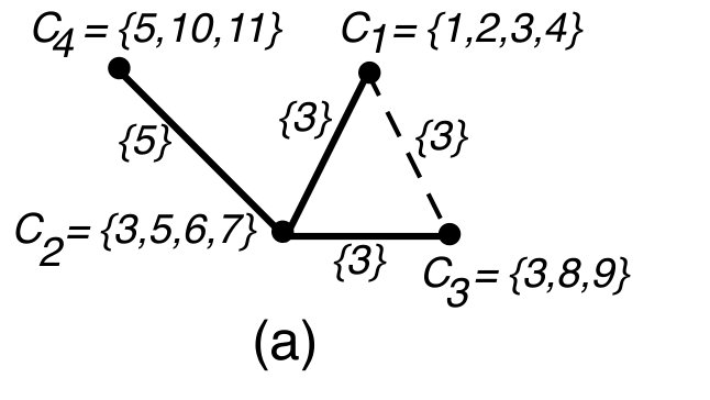 Figure 1
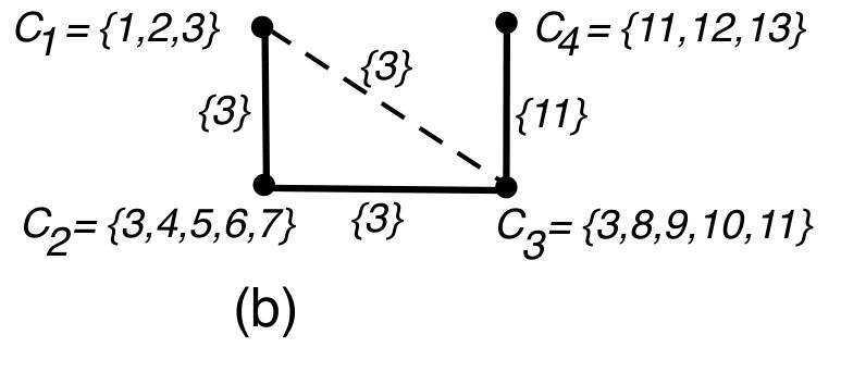 Figure 2
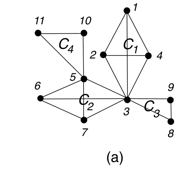 Figure 3
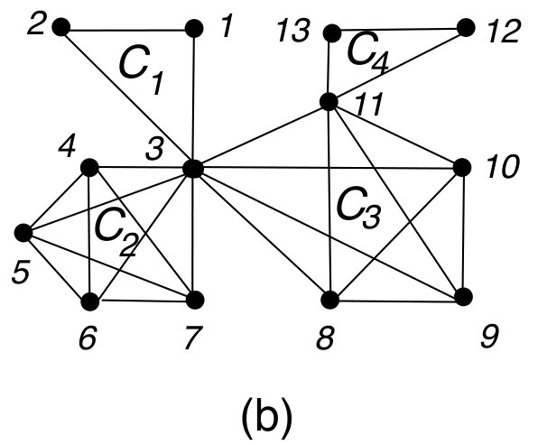 Figure 4
Peer Reviews
No public reviews on file for this paper yet. If you reviewed it on a platform where reviews are public (OpenReview, ICLR, NeurIPS, ICML), you can paste yours below so the community can read it here.
Videos
No videos yet. Explain this paper in a talk, walkthrough, or lecture? Add one.
Taxonomy
TopicsAdvanced Optimization Algorithms Research · Sparse and Compressive Sensing Techniques · Complexity and Algorithms in Graphs
Doubly nonnegative relaxations are equivalent to completely positive reformulations of
quadratic optimization problems with block-clique graph structures
Sunyoung Kim Department of Mathematics, Ewha W. University, 52 Ewhayeodae-gil, Sudaemoon-gu, Seoul 03760, Korea ([email protected]). The research was supported by NRF 2017-R1A2B2005119.
Masakazu Kojima Department of Industrial and Systems Engineering, Chuo University, Tokyo 192-0393, Japan ([email protected]). This research was supported by Grant-in-Aid for Scientific Research (A) 26242027.
Kim-Chuan Toh Department of Mathematics, and Institute of Operations Research and Analytics, National University of Singapore, 10 Lower Kent Ridge Road, Singapore 119076 ([email protected]). This research is supported in part by the Ministry of Education, Singapore, Academic Research Fund (Grant number: R-146-000-257-112).
Abstract
We study the equivalence among a nonconvex QOP, its CPP and DNN relaxations under the assumption that the aggregated and correlative sparsity of the data matrices of the CPP relaxation is represented by a block-clique graph . By exploiting the correlative sparsity, we decompose the CPP relaxation problem into a clique-tree structured family of smaller subproblems. Each subproblem is associated with a node of a clique tree of . The optimal value can be obtained by applying an algorithm that we propose for solving the subproblems recursively from leaf nodes to the root node of the clique-tree. We establish the equivalence between the QOP and its DNN relaxation from the equivalence between the reduced family of subproblems and their DNN relaxations by applying the known results on: (i) CPP and DNN reformulation of a class of QOPs with linear equality, complementarity and binary constraints in nonnegative variables. (ii) DNN reformulation of a class of quadratically constrained convex QOPs with any size. (iii) DNN reformulation of LPs with any size. As a result, we show that a QOP whose subproblems are the QOPs mentioned in (i), (ii) and (iii) is equivalent to its DNN relaxation, if the subproblems form a clique-tree structured family induced from a block-clique graph.
**Key words. ** Equivalence of doubly nonnegative relaxations and completely positive programs, sparsity of completely positive reformulations, aggregated and correlative sparsity, block clique graphs, completely positive and doubly nonnegative matrix completion, exact optimal values of nonconvex QOPs.
AMS Classification. 90C20, 90C26.
1 Introduction
Completely positive programming (CPP) relaxations of a class of quadratic optimization problems (QOPs) have received a great deal of attention as they can provide the optimal value of the original QOP [2, 7, 8, 17, etc.] even with their computational intractability. They are also referred as CPP reformulations of QOPs. As for computationally tractable alternatives, further relaxations of the CPP reformulations to doubly nonnegative programming (DNN) relaxations have been studied in [4, 16], and their effectiveness in obtaining good lower bounds for the optimal value of the QOP have been demonstrated in [14, 16]. Since the equivalence among QOPs, their CPP and DNN relaxations cannot be obtained in general, in this paper, we explore structured QOPs for which the equivalence to their DNN reformulations can be established. In particular, we focus on some structured sparsity characterized by block-clique graphs [9] and partial convexity to establish their equivalence for a class of QOPs. As far as we are aware of, this is the first time that the equivalence of nonconvex QOPs and their DNN relaxations are studied for this class of structured QOPs.
We start by introducing a conic optimization problem (COP) model to simultaneously represent QOPs, CPP problems and DNN problems. Let \mbox{\mathbb{R}}^{n} denote the -dimensional Euclidean space and \mbox{\mathbb{R}}^{n}_{+} the corresponding nonnegative orthant. We assume that each \mbox{\boldmathx}\in\mbox{\mathbb{R}}^{n} is a column vector, and \mbox{\boldmathx}^{T} denotes its transpose. Let \mbox{\mathbb{S}}^{n} denote the space of symmetric matrices. For every pair of \mbox{\boldmathA}\in\mbox{\mathbb{S}}^{n} and \mbox{\boldmathX}\in\mbox{\mathbb{S}}^{n}, \langle\mbox{\boldmathA},\,\mbox{\boldmathX}\rangle stands for their inner product defined as the trace of A$$X. Let and be disjoint finite subsets of positive integers and \mbox{\boldmathQ}^{p}\in\mbox{\mathbb{S}}^{n} . Given a closed (possibly nonconvex) cone \mbox{\mathbb{K}}\subset\mbox{\mathbb{S}}^{n}, we consider the following general COP:
[TABLE]
The distinctive feature of COP(\mbox{\mathbb{K}}) is that it only involves homogeneous equality and inequality constraints except . A general equality standard form COP can be transformed to COP(\mbox{\mathbb{K}}) with in a straightforward manner (see Section 2.2). If \mbox{\bf{\Gamma}}^{n}=\{\mbox{\boldmathx}\mbox{\boldmathx}^{T}\in\mbox{\mathbb{S}}^{n}:\mbox{\boldmathx}\in\mbox{\mathbb{R}}^{n}_{+}\} is chosen as the closed cone \mbox{\mathbb{K}}\subset\mbox{\mathbb{S}}^{n}, then COP(\mbox{\bf{\Gamma}}^{n}) represents a QOP with quadratic equality and inequality constraints in \mbox{\boldmathx}\in\mbox{\mathbb{R}}^{n}_{+} (see Section 2.5). Notice that the inequality constraints \langle\mbox{\boldmathQ}^{p},\,\mbox{\boldmathX}\rangle\leq 0\ (p\in I_{\rm ineq}) are dealt with separately from the equality constraints \langle\mbox{\boldmathQ}^{p},\,\mbox{\boldmathX}\rangle=0\ (p\in I_{\rm eq}) without introducing slack variables. In particular, the inequality constraints \langle\mbox{\boldmathQ}^{p},\,\mbox{\boldmathX}\rangle\leq 0\ (p\in I_{\rm ineq}) with \mbox{\boldmathX}\in\mbox{\bf{\Gamma}}^{n} correspond to convex quadratic inequality constraints in Section 2.5. If is the DNN cone of size (denoted as \mbox{\mathbb{DNN}}^{n}) or the CPP cone of size (denoted as \mbox{\mathbb{CPP}}^{n}), then COP(\mbox{\mathbb{K}}) represents a general DNN or CPP problem, respectively (see Section 2.2). They are known to serve as convex relaxations of the nonconvex QOP, COP(\mbox{\bf{\Gamma}}^{n}). In general, \zeta(\mbox{\mathbb{DNN}}^{n})\leq\zeta(\mbox{\mathbb{CPP}}^{n})\leq\zeta(\mbox{\bf{\Gamma}}^{n}) holds since \mbox{\bf{\Gamma}}^{n}\subset\mbox{\mathbb{CPP}}^{n}\ \mbox{(=\mbox{}^{n})}\subset\mbox{\mathbb{DNN}}^{n}.
The main purpose of this paper is to investigate structured sparsity, in particular, the aggregated sparsity [12] and the correlative sparsity [18] characterized by block-clique graphs [9], and partial convexity of the data matrices of COP(\mbox{\mathbb{K}}) to establish the equivalence among the three types of problems, COP(\mbox{\bf{\Gamma}}^{n}), COP(\mbox{\mathbb{CPP}}^{n}) and COP(\mbox{\mathbb{DNN}}^{n}).
Sparsity, especially the chordal graph sparsity, has been heavily used to improve the computational efficiency of solving semidefinite programming (SDP) problems. The sparsity exploitation technique [12, 18, 20, 21, etc.] for SDP problems was based on the semidefinite matrix completion in order to reduce the size of the positive semidefinite variable matrix. More precisely, it replaces a large but sparse variable matrix of a given SDP problem with smaller positive semidefinite variable matrices whose sizes are determined by the maximal cliques of the extended chordal graph characterizing the aggregated sparsity of the data matrices of the SDP problem. On the other hand, exploiting sparsity in CPP problems has not been studied in the literature, to the best of our knowledge, as the studies on CPP problems have been mainly for theoretical interests.
We discuss the equivalence of COP(\mbox{\bf{\Gamma}}^{n}), COP(\mbox{\mathbb{CPP}}^{n}) and COP(\mbox{\mathbb{DNN}}^{n}) based on the following techniques and/or facts.
(a) The CPP and DNN matrix completion in [10].
(b) Exploiting (aggregated and correlative) sparsity in chordal graph structured SDPs [12, 18].
(c) \mbox{\mathbb{CPP}}^{n}=\mbox{\mathbb{DNN}}^{n} if .
(d) CPP reformulation of a class of QOPs with linear equality, binary and complementarity constraints [2, 7, 8, 17, etc.].
(e) DNN reformulation of quadratically constrained convex QOPs in nonnegative variables. See Lemma 2.5 in Section 2.6.
We note that (c) is well-known. A block-clique graph is a chordal graph in which any two maximal cliques intersect in at most one vertex [9]. It was shown in [10] that every partial CPP (or DNN) matrix whose specified entries are determined by an undirected graph has a CPP (or DNN) completion if and only if is a block-clique graph.
Let \mbox{\mathbb{K}}\in\{\mbox{\bf{\Gamma}}^{n},\mbox{\mathbb{CPP}}^{n},\mbox{\mathbb{DNN}}^{n}\}. In our method, the basic idea developed in (b) combined with (a), instead of positive semidefinite matrix completion [13], is applied to COP(\mbox{\mathbb{K}}) with \mbox{\boldmathQ}^{p}\in\mbox{\mathbb{S}}^{n} . The data structure of COP(\mbox{\mathbb{K}}) is characterized by a block-clique graph with the maximal cliques . COP(\mbox{\mathbb{K}}) is then decomposed into a family of smaller size subproblems according to a clique tree structure induced from . The family of subproblems inherit the clique tree structure of the block-clique graph . More precisely, they are associated with the nodes of the clique tree. Two distinct subproblems are almost independent but weakly connected in the sense that they share one scalar variable if they are adjacent in the clique tree and no common variable otherwise. In addition, each problem associated with a clique in the family is of the same form as COP(\mbox{\mathbb{K}}), but the size of its matrix variable is decreased to the size of . It is important to note that the decomposition is independent of the choice of \mbox{\mathbb{K}}\in\{\mbox{\bf{\Gamma}}^{n},\mbox{\mathbb{CPP}}^{n},\mbox{\mathbb{DNN}}^{n}\}.
We utilize the aforementioned decomposition of COP() for two purposes: to efficiently solve large scale COPs and to show the equivalence among COP(\mbox{\bf{\Gamma}}^{n}), COP(\mbox{\mathbb{CPP}}^{n}) and COP(\mbox{\mathbb{DNN}}^{n}). For the first purpose of efficiently solving large scale COPs, the optimal value \zeta(\mbox{\mathbb{K}}) of COP() is computed by solving the small decomposed subproblems in the family. We propose an algorithm for sequentially solving the decomposed subproblems. As a result, the proposed algorithm is more efficient than directly solving the original COP() when its size becomes increasingly large. Here we implicitly assume that \mbox{\mathbb{K}}=\mbox{\mathbb{DNN}}^{n}, although all the results would remain valid even when the decomposed subproblems are not numerically tractable. We should emphasize that the decomposition into smaller subproblems is certainly beneficial computationally. For example, the decomposition of a DNN problem of size 1000 into DNN subproblems of size at most is certainly much more numerically tractable than the original DNN problem.
For the second purpose of showing the equivalence among COP(\mbox{\bf{\Gamma}}^{n}), COP(\mbox{\mathbb{CPP}}^{n}) and COP(\mbox{\mathbb{DNN}}^{n}), the decomposition is applied to a pair of COP(\mbox{\mathbb{K}}_{1}) and COP(\mbox{\mathbb{K}}_{2}) with two distinct \mbox{\mathbb{K}}_{1},\ \mbox{\mathbb{K}}_{2}\in\{\mbox{\bf{\Gamma}}^{n},\mbox{\mathbb{CPP}}^{n},\mbox{\mathbb{DNN}}^{n}\}. Then, two families of subproblems, say family from COP(\mbox{\mathbb{K}}_{1}) and family from COP(\mbox{\mathbb{K}}_{2}), are obtained. The equivalence between COP(\mbox{\mathbb{K}}_{1}) and COP(\mbox{\mathbb{K}}_{2}) is reduced to the equivalence of family and family . We note that a pair of decomposed subproblems, one from family and the other form family 2, associated with a common clique share the common objective function and constraints except for their cone constraints. Thus, (c), (d) and/or (e) can be applied for the equivalence of each pair. If all pairs of subproblems from families and are equivalent, then COP(\mbox{\mathbb{K}}_{1}) and COP(\mbox{\mathbb{K}}_{2}) are equivalent. In particular, all of nonconvex QOPs with linear and complementarity constraints in variables, quadratically constrained convex QOPs with any size and LPs with any size can be included as subproblems in a single QOP formulated as COP(\mbox{\bf{\Gamma}}), which can then be equivalently reformulated as its DNN relaxation. We should mention that a structured sparsity, i.e., the aggregate and correlative sparsity characterized by a block-clique graph, needs to be imposed on the QOP. Such a QOP may not appear frequently in practice, but our study here has theoretical importance as nonconvex QOPs are NP hard to solve in general.
This paper is organized as follows: In Section 2, some basics on block-clique graphs, (a), (c), (d) and (e) are described. We also define the aggregate and correlative sparsity which are represented by an undirected graph. Sections 3 and 4 include the main results of this paper. In Section 3, the equivalence among COP(\mbox{\bf{\Gamma}}^{n}), COP(\mbox{\mathbb{CPP}}^{n}) and COP(\mbox{\mathbb{DNN}}^{n}) based on (c) and (d) is established by exploiting the aggregated sparsity characterized by block-clique graphs. In Section 4, we show how COP(\mbox{\mathbb{K}}) with \mbox{\mathbb{K}}\in\{\mbox{\bf{\Gamma}}^{n},\mbox{\mathbb{CPP}}^{n},\mbox{\mathbb{DNN}}^{n}\} can be decomposed into smaller subproblems by exploiting the correlative sparsity. Then the equivalence results given in Section 3 as well as (e) are applied to a pair of subproblems induced from distinct COP(\mbox{\mathbb{K}}_{1}) and COP(\mbox{\mathbb{K}}_{2}) to verify their equivalence as mentioned above. We also present an algorithm to sequentially solve smaller decomposed subproblems. In Section 5, we illustrate two types of QOPs, block-clique graph structured QOPs with linear equality and complementarity constraints and partially convex QOPs, which can be formulated as the equivalent DNN problems. We conclude the paper in Section 6.
2 Preliminaries
2.1 Notation and symbols
We will consider the following cones in \mbox{\mathbb{S}}^{n}.
[TABLE]
The following relation is well-known [5]:
[TABLE]
Let . For each nonempty subset of , \mbox{\mathbb{R}}^{C} denotes the -dimensional Euclidean space of column vectors of , and \mbox{\mathbb{S}}^{C} the linear space of symmetric matrices consisting of the elements . A vector in \mbox{\mathbb{R}}^{C} denoted by \mbox{\boldmathx}_{C} is regarded as a subvector of \mbox{\boldmathx}\in\mbox{\mathbb{R}}^{n}, and a matrix in \mbox{\mathbb{S}}^{C} denoted by \mbox{\boldmathX}_{C} as a principal submatrix of \mbox{\boldmathX}\in\mbox{\mathbb{S}}^{n}. We define \mbox{\bf{\Gamma}}^{C}=\left\{\mbox{\boldmathx}_{C}\mbox{\boldmathx}_{C}^{T}:\mbox{\boldmathx}_{C}\in\mbox{\mathbb{R}}^{C}_{+}\right\}, and \mbox{\mathbb{DNN}}^{C} and \mbox{\mathbb{CPP}}^{C} to be the DNN cone and the CPP cone in \mbox{\mathbb{S}}^{C}, respectively.
We say a subset of symmetric if it satisfies . For every symmetric subset of , we denote and by and , respectively.
2.2 Conversion of general COPs to COP(\mbox{\mathbb{K}})
Let d_{p}\in\mbox{\mathbb{R}} and \overline{\mbox{\boldmathQ}}^{p}\in\mbox{\mathbb{S}}^{n} . We assume . For each \mbox{\mathbb{K}}\in\{\mbox{\bf{\Gamma}}^{n},\mbox{\mathbb{CPP}}^{n},\mbox{\mathbb{DNN}}^{n}\}, consider a general COP in the standard equality form:
[TABLE]
Let , and \mbox{\boldmathQ}^{p}=\begin{pmatrix}-d_{p}&\mbox{\bf 0}^{T}\\ \mbox{\bf 0}&\overline{\mbox{\boldmathQ}}^{p}\end{pmatrix}\in\mbox{\mathbb{S}}^{1+n}\ (p=0,1,\ldots,m). Then \langle\mbox{\boldmathQ}^{p},\,\mbox{\boldmathX}\rangle=\langle\overline{\mbox{\boldmathQ}}^{p},\,\mbox{\boldmathY}\rangle-d_{p}X_{11} for every \mbox{\boldmathX}=\begin{pmatrix}X_{11}&\mbox{\boldmathx}^{T}\\ \mbox{\boldmathx}&\mbox{\boldmathY}\end{pmatrix}\in\mbox{\mathbb{S}}^{1+n} . Therefore, the above standard equality form COP with \mbox{\mathbb{K}}=\mbox{\bf{\Gamma}}^{n}, \mbox{\mathbb{K}}=\mbox{\mathbb{CPP}}^{n} and \mbox{\mathbb{K}}=\mbox{\mathbb{DNN}}^{n} can be rewritten as COP(\mbox{\bf{\Gamma}}^{1+n}), COP(\mbox{\mathbb{CPP}}^{1+n}) and COP(\mbox{\mathbb{DNN}}^{1+n}), respectively. Conversely, if slack variables are introduced for the inequality constraints \langle\mbox{\boldmathQ}^{p},\,\mbox{\boldmathX}\rangle\leq 0 in COP(\mbox{\mathbb{K}}), COP(\mbox{\mathbb{K}}) can be converted into the standard equality form COP in a straightforward fashion.
2.3 Chordal and block-clique graphs
We consider an undirected graph with the node set and the edge set . Here is a symmetric subset of (hence ) and is identified with . A graph is called chordal if every cycle in of length or more has a chord, and block-clique [9] if it is a chordal graph and any pair of two maximal cliques of intersects in at most one node. See Figure 1 for examples of block-clique graphs.
Let be a chordal graph with the maximal cliques . We assume that the graph is connected. If it is not, the subsequent discussion can be applied to each connected component. Consider an undirected graph on the maximal cliques, G(\mbox{\cal N},\mbox{\cal E}) with the node set and the edge set \mbox{\cal E}=\{(C_{q},C_{r}):C_{q}\cap C_{r}\not=\emptyset\}. Since is assumed to be connected, G(\mbox{\cal N},\mbox{\cal E}) is connected. Then, add the weight to each edge (C_{q},C_{r})\in\mbox{\cal E}. Here denotes the number of nodes contained in the clique . It is known that every maximum weight spanning tree G(\mbox{\cal N},\mbox{\cal T}) of G(\mbox{\cal N},\mbox{\cal E}) satisfies the following clique intersection property:
[TABLE]
Such a tree is called as a clique tree of . We refer to [6] for the fundamental properties of chordal graphs and clique trees including the clique intersection property and the running intersection property described below.
Now suppose that is a connected block-clique graph. Then we know that if (C_{q},C_{r})\in\mbox{\cal E}. Hence, every spanning tree of G(\mbox{\cal N},\mbox{\cal E}) is a clique tree. See Figure 2. Let G(\mbox{\cal N},\mbox{\cal T}) be a clique tree of . Choose an arbitrary maximal clique as a root node, say . The rest of the maximal cliques can be renumbered such that for any pair of distinct and , if is on the (unique) path from the root node to then holds by applying a topological sorting (ordering). In this way, the renumbered sequence of maximal cliques satisfies *the running intersection property: *
[TABLE]
Let , and the (unique) parent of . Then and
[TABLE]
for some . If satisfies in the running intersection property above, then
[TABLE]
Here, the last equality follows from the assumption that . Therefore, we have shown the following result.
Lemma 2.1**.**
(The running intersection property applied to a block-clique graph.) Let be a connected block-clique graph with the maximal cliques . Choose one of the maximal cliques arbitrary, say . Then, the rest of the maximal cliques can be renumbered such that
[TABLE]
holds.
2.4 Matrix completion
We call an matrix array a partial symmetric matrix if a part of its elements are specified for some symmetric and the other elements are not specified. We denote a partial symmetric matrix with specified elements by . Given a property P characterizing a symmetric matrix in \mbox{\mathbb{S}}^{n} and a partial symmetric matrix for some symmetric , the matrix completion problem with property P is to find values of unspecified elements such that the resulting symmetric matrix \bar{\mbox{\boldmathX}} has property P. We say that the partial symmetric matrix has a completion \bar{\mbox{\boldmathX}} with property P.
We mainly consider CPP and DNN matrices in the subsequent discussions. In these matrices, we may assume without loss of generality that since unspecified diagonal elements can be given as sufficiently large positive values to realize the property. Each partial symmetric matrix can be associated with a graph . (Recall that .) Let be the maximal cliques of . Then the partial symmetric matrix is decomposed into partial symmetric matrices , which can be consistently described as \bar{\mbox{\boldmathX}}_{C_{q}}, . We say that a partial symmetric matrix is partially DNN (partially CPP) if every \bar{\mbox{\boldmathX}}_{C_{q}} is DNN (CPP, respectively) in \mbox{\mathbb{S}}^{C_{q}} .
Lemma 2.2**.**
[10]** Let be a symmetric subset of such that for every . Then every partial CPP (DNN) matrix has a CPP (DNN, respectively) completion, i.e., a CPP (DNN, respectively) matrix such that , iff is a block clique graph.
2.5 A class of QOPs and their CPP and DNN relaxations
Any quadratic function in nonnegative variables can be represented as \langle\mbox{\boldmathQ},\,\mbox{\boldmathx}\mbox{\boldmathx}^{T}\rangle with \mbox{\boldmathx}=(x_{1},x_{2},\ldots,x_{n})\in\mbox{\mathbb{R}}^{n}_{+} and for some \mbox{\boldmathQ}\in\mbox{\mathbb{S}}^{n}. By introducing a variable matrix \mbox{\boldmathX}\in\mbox{\bf{\Gamma}}^{n}\equiv\{\mbox{\boldmathx}\mbox{\boldmathx}^{T}:\mbox{\boldmathx}\in\mbox{\mathbb{R}}^{n}_{+}\}, the function can be rewritten as \langle\mbox{\boldmathQ},\,\mbox{\boldmathX}\rangle with . As a result, a general quadratically constrained QOP in nonnegative variables can also be represented as COP(\mbox{\bf{\Gamma}}^{n}) introduced in Section 1. Since \mbox{\bf{\Gamma}}^{n}\subset\mbox{\mathbb{CPP}}^{n}\subset\mbox{\mathbb{DNN}}^{n}, \zeta(\mbox{\mathbb{DNN}}^{n})\leq\zeta(\mbox{\mathbb{CPP}}^{n})\leq\zeta(\mbox{\bf{\Gamma}}^{n}) holds in general.
On the equivalence between QOPs and their CPP relaxations, Burer’s reformulation [8] for a class of QOPs with linear constraints in nonnegative and binary variables is well-known. In this paper, we employ the following result, which is essentially equivalent to Burer’s reformulation. See [17] for CPP reformulations of more general class of QOPs.
Lemma 2.3**.**
[3, Theorem 3.1]** For COP(\mbox{\bf{\Gamma}}^{n}), assume that
[TABLE]
Then, \zeta(\mbox{\bf{\Gamma}}^{n})=\zeta(\mbox{\mathbb{CPP}}^{n}).
Example 2.4**.**
Let be a matrx, and \mbox{\boldmathQ}^{0}\in\mbox{\mathbb{S}}^{n}. Consider a QOP with linear equality and complementarity constraints in nonnegative variables \mbox{\boldmathx}\in\mbox{\mathbb{R}}^{n}_{+}.
[TABLE]
Define
[TABLE]
Then, the QOP can be rewritten as
[TABLE]
Enumerate from through some integer , and let and . Then QOP can be rewritten as COP(\mbox{\bf{\Gamma}}^{n}). Obviously \mbox{\boldmathQ}^{1}\in\mbox{\mathbb{S}}^{n}_{+} and \mbox{\boldmathQ}^{ij}\in\mbox{\mathbb{N}}^{n} . Hence, if the QOP is feasible and \mbox{\boldmathO}=\{\mbox{\boldmathX}\in\mbox{\bf{\Gamma}}^{m}:X_{11}=0,\ \langle\mbox{\boldmathQ}^{1},\,\mbox{\boldmathX}\rangle=0\}=\{\mbox{\boldmathx}\mbox{\boldmathx}^{T}:\mbox{\boldmathx}\in\mbox{\mathbb{R}}^{n}_{+},\ x_{1}=0,\ \mbox{\boldmathA}\mbox{\boldmathx}=\mbox{\bf 0}\}, then all the assumptions in Lemma 2.3 are satisfied. Consequently, \zeta(\mbox{\bf{\Gamma}}^{n})=\zeta(\mbox{\mathbb{CPP}}^{n}) holds. We note that the binary condition on variable can be represented as , and with a slack variable . Thus, binary variables can be included in the QOP above. This QOP model covers various combinatorial optimization problems. See [3, 16] for more details.
It is well-known that a convex QOP can be reformulated as an SDP (see, for example, [11]). The following result may be regarded as a variation of the SDP reformulation to CPP and DNN reformulations of a convex QOP in nonnegative variables.
Lemma 2.5**.**
Let . Assume that \mbox{\boldmathQ}^{0}_{\widetilde{N}}\in\mbox{\mathbb{S}}^{n-1}_{+}, \mbox{\boldmathQ}^{p}\in\mbox{\mathbb{S}}^{n}_{+} and \mbox{\boldmathQ}^{p}_{\widetilde{N}}\in\mbox{\mathbb{S}}^{n-1}_{+} . Then \zeta(\mbox{\mathbb{DNN}}^{n})=\zeta(\mbox{\mathbb{CPP}}^{n})=\zeta(\mbox{\bf{\Gamma}}^{n}). Furthermore, if \mbox{\boldmathX}=\begin{pmatrix}1&\mbox{\boldmathy}^{T}\\ \mbox{\boldmathy}&\mbox{\boldmathY}\end{pmatrix}\in\mbox{\mathbb{DNN}}^{n} with some \mbox{\boldmathy}\in\mbox{\mathbb{R}}^{n-1}_{+} and \mbox{\boldmathY}\in\mbox{\mathbb{DNN}}^{n-1} is an optimal solution of COP(\mbox{\mathbb{DNN}}^{n}), then \begin{pmatrix}1&\mbox{\boldmathy}^{T}\\ \mbox{\boldmathy}&\mbox{\boldmathy}\mbox{\boldmathy}^{T}\end{pmatrix} is a common optimal solution of COP(\mbox{\bf{\Gamma}}^{n}), COP(\mbox{\mathbb{CPP}}^{n}) and COP(\mbox{\mathbb{DNN}}^{n}) with the objective value \zeta(\mbox{\mathbb{DNN}}^{n})=\zeta(\mbox{\mathbb{CPP}}^{n})=\zeta(\mbox{\bf{\Gamma}}^{n}).
Proof.
The inequality \zeta(\mbox{\mathbb{DNN}}^{n})\leq\zeta(\mbox{\mathbb{CPP}}^{n})\leq\zeta(\mbox{\bf{\Gamma}}^{n}) follows from \mbox{\bf{\Gamma}}^{n}\subset\mbox{\mathbb{CPP}}^{n}\subseteq\mbox{\mathbb{DNN}}^{n}. It suffices to show \zeta(\mbox{\bf{\Gamma}}^{n})\leq\zeta(\mbox{\mathbb{DNN}}^{n}). Let \mbox{\boldmathX}=\begin{pmatrix}1&\mbox{\boldmathy}^{T}\\ \mbox{\boldmathy}&\mbox{\boldmathY}\end{pmatrix}\in\mbox{\mathbb{DNN}}^{n} with some \mbox{\boldmathy}\in\mbox{\mathbb{R}}^{n-1}_{+} and \mbox{\boldmathY}\in\mbox{\mathbb{DNN}}^{n-1} be an arbitrary feasible solution of COP(\mbox{\mathbb{DNN}}^{n}). Then,
[TABLE]
From the last inequality, the assumptions and \overline{\mbox{\boldmathX}}\in\mbox{\mathbb{CPP}}^{n}\subset\mbox{\mathbb{S}}^{n}_{+}, we see that
[TABLE]
Thus we have shown that \overline{\mbox{\boldmathX}} is a feasible solution of COP(\mbox{\bf{\Gamma}}^{n}) whose objective value is not greater than that of the feasible solution of COP(\mbox{\mathbb{DNN}}^{n}). Therefore \zeta(\mbox{\bf{\Gamma}}^{n})\leq\zeta(\mbox{\mathbb{DNN}}^{n}) has been shown. The second assertion follows by choosing an optimal solution of COP(\mbox{\mathbb{DNN}}^{n}) for in the proof above. ∎
Example 2.6**.**
(Quadratically constrained convex QOPs) Let and . Let be a matrx and \mbox{\boldmathQ}^{p}\in\mbox{\mathbb{S}}^{n} be such that \mbox{\boldmathQ}^{0}_{\widetilde{N}}\in\mbox{\mathbb{S}}^{\widetilde{N}}_{+} . Consider a QOP:
[TABLE]
which represents a general quadratically constrained convex QOP in nonnegative variables . If we let \mbox{\boldmathQ}^{1}=\mbox{\boldmathA}^{T}\mbox{\boldmathA}\in\mbox{\mathbb{S}}^{n}_{+} and , we can represent the QOP as COP(\mbox{\bf{\Gamma}}^{n}). By Lemma 2.5, not only \zeta(\mbox{\mathbb{DNN}}^{n})=\zeta(\mbox{\mathbb{CPP}}^{n})=\zeta(\mbox{\bf{\Gamma}}^{n}) holds, but also the DNN relaxation provides an optimal solution of the QOP.
2.6 Two types of sparsity
We consider two types of sparsity of the data matrices \mbox{\boldmathQ}^{p} of COP(\mbox{\mathbb{K}}) with \mbox{\mathbb{K}}\in\{\mbox{\bf{\Gamma}}^{n},\mbox{\mathbb{CPP}}^{n},\mbox{\mathbb{DNN}}^{n}\}, the aggregated sparsity [12] and the correlative sparsity [18]. We say that the aggregated sparsity of matrices \mbox{\boldmathA}^{p}\in\mbox{\mathbb{S}}^{n} is represented by a graph if for every , and that their correlative sparsity is represented by a graph with the maximal cliques if
[TABLE]
Note that if are the maximal cliques of , then . We also note that a graph which represents the aggregate (correlative) sparsity of \mbox{\boldmathA}^{p}\in\mbox{\mathbb{S}}^{n} is not unique.
Our main interest in the subsequent discussion is a block-clique graph which represents the aggregate (correlative) sparsity of \mbox{\boldmathA}^{p}\in\mbox{\mathbb{S}}^{n} . If we let , then is “the smallest” graph which represents their aggregate sparsity. Since it is not block-clique in general, a block-clique extension of is necessary. Assume that is connected. It is straightforward to verify that a node of a connected block-clique graph is a cut node iff it is contained in at least two distinct maximal cliques of the graph. Therefore, if there exists no cut node in , then the complete graph is the only block-clique extension of . Otherwise, take the maximal edge set such that the graph has the same cut nodes as . Then forms the smallest block-clique extension of .
Obviously, if a graph represents the correlative sparsity of matrices \mbox{\boldmathA}^{p}\in\mbox{\mathbb{S}}^{n} , then it also represents their aggregate sparsity. But the converse is not true as we see in the following example.
Example 2.7**.**
Let , and
[TABLE]
where * denotes a nonzero element. We see that the aggregate sparsity pattern of the two matrices \mbox{\boldmathA}^{1} and \mbox{\boldmathA}^{2} corresponds to \overline{\mbox{\boldmathA}}. Thus their aggregated sparsity is represented by the graph with the maximal cliques and . But neither nor covers the nonzero elements of \mbox{\boldmathA}^{1}. We need to take the complete graph with the single maximal clique to represent the correlative sparsity of \mbox{\boldmathA}^{1} and \mbox{\boldmathA}^{2}.
3 Exploiting the aggregated sparsity characterized by block-clique graphs
Throughout this section, we assume that the aggregate sparsity of the data matrices \mbox{\boldmathQ}^{p} of COP() with \mbox{\mathbb{K}}\in\{\mbox{\bf{\Gamma}}^{n},\mbox{\mathbb{CPP}}^{n},\mbox{\mathbb{DNN}}^{n}\} is represented by a block-clique graph ;
[TABLE]
Under this assumption, we provide sufficient conditions for \zeta(\mbox{\mathbb{DNN}}^{n})=\zeta(\mbox{\mathbb{CPP}}^{n}) and \zeta(\mbox{\bf{\Gamma}}^{n})=\zeta(\mbox{\mathbb{DNN}}^{n})=\zeta(\mbox{\mathbb{CPP}}^{n}).
Note that the values of elements determine the value of \langle\mbox{\boldmathQ}^{p},\,\mbox{\boldmathX}\rangle, i.e., \langle\mbox{\boldmathQ}^{p},\,\mbox{\boldmathX}\rangle=\sum_{(i,j)\in\overline{E}}Q^{p}_{ij}X_{ij} . All other elements affect only the cone constraint \mbox{\boldmathX}\in\mbox{\mathbb{K}} in COP(). Thus, the cone constraint can be replaced by “ has a completion \mbox{\boldmathX}\in\mbox{\mathbb{K}}”. More precisely, COP() can be written as
[TABLE]
Let be the maximal cliques of . We now introduce a (sparse) relaxation of COP (17) ( COP()).
[TABLE]
Since we have been dealing with the case where \mbox{\mathbb{K}}\in\{\mbox{\bf{\Gamma}}^{n},\mbox{\mathbb{CPP}}^{n},\mbox{\mathbb{DNN}}^{n}\}, \mbox{\mathbb{K}}^{C_{q}} stands for \mbox{\bf{\Gamma}}^{C_{q}}, \mbox{\mathbb{DNN}}^{C_{q}} or \mbox{\mathbb{CPP}}^{C_{q}} . In either case, \mbox{\boldmathX}\in\mbox{\mathbb{K}} implies \mbox{\boldmathX}_{C_{q}}\in\mbox{\mathbb{K}}^{C_{q}} . Thus COP (21) serves as a relaxation of COP (17); \eta(\mbox{\mathbb{K}})\leq\zeta(\mbox{\mathbb{K}}).
Theorem 3.1**.**
Let \mbox{\mathbb{K}}\in\{\mbox{\bf{\Gamma}}^{n},\mbox{\mathbb{CPP}}^{n},\mbox{\mathbb{DNN}}^{n}\}. Assume that (13) holds for a block-clique graph with the maximal cliques . Then,
(i) \eta(\mbox{\mathbb{K}})=\zeta(\mbox{\mathbb{K}}).
(ii) If every clique contains at most nodes , then COP (21) with \mbox{\mathbb{K}}=\mbox{\mathbb{CPP}}^{n} and COP (21) with \mbox{\mathbb{K}}=\mbox{\mathbb{DNN}}^{n} are equivalent; more precisely they share the same feasible solutions, the optimal solutions and the optimal value \eta(\mbox{\mathbb{CPP}}^{n})=\eta(\mbox{\mathbb{DNN}}^{n}).
(iii) If every clique contains at most nodes and the assumptions of Lemma 2.3 are satisfied, then \eta(\mbox{\bf{\Gamma}}^{n})=\zeta(\mbox{\bf{\Gamma}}^{n})=\zeta(\mbox{\mathbb{CPP}}^{n})=\eta(\mbox{\mathbb{CPP}}^{n})=\eta(\mbox{\mathbb{DNN}}^{n}).
Proof.
(i) Suppose that \mbox{\mathbb{K}}\in\{\mbox{\mathbb{DNN}}^{n},\mbox{\mathbb{CPP}}^{n}\}. By Lemma 2.2, the condition “[X_{ij}:(i,j)\in\overline{E}]\ \mbox{has a completion }\mbox{\boldmathX}\in\mbox{\mathbb{K}}” in COP (17) is equivalent to the condition “\mbox{\boldmathX}_{C_{q}}\in\mbox{\mathbb{K}}^{C_{q}}\ (q=1,\ldots,\ell)” in COP (21). Hence COPs (17) and (21) are equivalent, which implies that \eta(\mbox{\mathbb{K}})=\zeta(\mbox{\mathbb{K}}). Now suppose that \mbox{\mathbb{K}}=\mbox{\bf{\Gamma}}^{n}. Since we already know that \eta(\mbox{\bf{\Gamma}}^{n})\leq\zeta(\mbox{\bf{\Gamma}}^{n}), it suffices to show that \zeta(\mbox{\bf{\Gamma}}^{n})\leq\eta(\mbox{\bf{\Gamma}}^{n}). Choose a maximal clique that contains node among , say . By Lemma 2.1, we can renumber the rest of the maximal cliques such that the running intersection property (10) holds. Assume that (\mbox{\boldmathX}_{C_{1}},\ldots,\mbox{\boldmathX}_{C_{\ell}}) is a feasible solution of COP (21) with \mbox{\mathbb{K}}=\mbox{\bf{\Gamma}}^{n}. We will construct an \bar{\mbox{\boldmathx}}\in\mbox{\mathbb{R}}^{n}_{+} such that \overline{\mbox{\boldmathX}}\equiv\bar{\mbox{\boldmathx}}\bar{\mbox{\boldmathx}}^{T} is a feasible solution of COP(\mbox{\bf{\Gamma}}^{n}) with the same objective value of COP (21) with \mbox{\mathbb{K}}=\mbox{\bf{\Gamma}}^{n} at its feasible solution (\mbox{\boldmathX}_{C_{1}},\ldots,\mbox{\boldmathX}_{C_{\ell}}). Then \zeta(\mbox{\bf{\Gamma}}^{n})\leq\eta(\mbox{\bf{\Gamma}}^{n}) follows. For each , there exists an \mbox{\boldmathy}_{C_{r}}\in\mbox{\mathbb{R}}^{C}_{+} such that \mbox{\boldmathX}_{C_{r}}=\mbox{\boldmathy}_{C_{r}}\mbox{\boldmathy}_{C_{r}}^{T}. For , let \bar{x}_{i}=[\mbox{\boldmathy}_{C_{1}}]_{i} . By (10), for each , there exists a such that . Hence, if we define \bar{x}_{i}=[\mbox{\boldmathy}_{C_{r}}]_{i}\ (i\in C_{r}\backslash\{k_{r}\}) for , then \bar{\mbox{\boldmathx}}\in\mbox{\mathbb{R}}^{n}_{+} satisfies \bar{x}_{i}=[\mbox{\boldmathy}_{C_{r}}]_{i}\ (i\in C_{r},r\in\{1,\ldots,\ell\}) and \overline{\mbox{\boldmathX}}=\bar{\mbox{\boldmathx}}\bar{\mbox{\boldmathx}}^{T}\in\mbox{\bf{\Gamma}}^{n} is a completion of . By construction, \overline{\mbox{\boldmathX}} is a feasible solution of COP(\mbox{\bf{\Gamma}}^{n}), and attains the same objective value of COP (21) with \mbox{\mathbb{K}}=\mbox{\bf{\Gamma}}^{n} at its feasible solution (\mbox{\boldmathX}_{C_{1}},\ldots,\mbox{\boldmathX}_{C_{\ell}}).
(ii) By (4), \mbox{\mathbb{CPP}}^{C_{q}}=\mbox{\mathbb{DNN}}^{C_{q}} , which implies the equivalence of COP (21) with \mbox{\mathbb{K}}=\mbox{\mathbb{CPP}}^{n} and COP (21) with \mbox{\mathbb{K}}=\mbox{\mathbb{DNN}}^{n}.
(iii) The identity \zeta(\mbox{\bf{\Gamma}}^{n})=\zeta(\mbox{\mathbb{CPP}}^{n}) follows from Lemma 2.3, and all other identities from (i) and (ii). ∎
To decompose the COP (21) based on the maximal cliques , we first decompose each \mbox{\boldmathQ}^{p} such that
[TABLE]
(We note that the decomposition of \mbox{\boldmathQ}^{p} above is not unique.) Then COP (21) can be represented as
[TABLE]
Remark 3.2**.**
(a) Note that under the assumption (13), if \mbox{\boldmathQ}^{p}\in\mbox{\mathbb{S}}^{n}_{+} (or \mbox{\boldmathQ}^{p}\in\mbox{\mathbb{S}}^{n}_{+}+\mbox{\mathbb{N}}^{n}), then we can take \widehat{\mbox{\boldmathQ}}^{pq}\in\mbox{\mathbb{S}}^{n}_{+} (or \widehat{\mbox{\boldmathQ}}^{pq}\in\mbox{\mathbb{S}}^{n}_{+}+\mbox{\mathbb{N}}^{n}) for the decomposition; see [1, Theorem 2.3]. In this case, the equality constraints \sum_{q=1}^{\ell}\langle\widehat{\mbox{\boldmathQ}}^{pq}_{C_{q}},\,\mbox{\boldmathX}_{C_{q}}\rangle=0\ (p\in I_{\rm eq}) can be replaced by \langle\widehat{\mbox{\boldmathQ}}^{pq}_{C_{q}},\,\mbox{\boldmathX}_{C_{q}}\rangle=0\ (q=1,\ldots,\ell,p\in I_{\rm eq}) since \langle\widehat{\mbox{\boldmathQ}}^{pq}_{C_{q}},\,\mbox{\boldmathX}_{C_{q}}\rangle\geq 0 for every \mbox{\boldmathX}\in\mbox{\mathbb{K}}\in\{\mbox{\bf{\Gamma}}^{n},\mbox{\mathbb{CPP}}^{n},\mbox{\mathbb{DNN}}^{n}\} is known.
(b) Suppose that form a partition of ; and . Then we have \widehat{\mbox{\boldmathQ}}^{pq}_{C_{q}}=\mbox{\boldmathQ}^{p}_{C_{q}} . In particular, if , then COP (25) turns out to be an LP of the form
[TABLE]
Here \mbox{\bf{\Gamma}}^{1}=\mbox{\mathbb{CPP}}^{1}=\mbox{\mathbb{DNN}}^{1}=\mbox{\mathbb{R}}_{+}. Although this observation itself is trivial, it is important in the sense that LPs can be embedded as subproblems in a QOP that can be reformulated as its DNN relaxations, as we will see in (v) of Theorem 4.6 and Section 5.2. **
4 Exploiting correlative sparsity characterized by block-clique graphs
We consider COP(\mbox{\mathbb{K}}) with \mbox{\mathbb{K}}\in\{\mbox{\bf{\Gamma}}^{n},\mbox{\mathbb{CPP}}^{n},\mbox{\mathbb{DNN}}^{n}\}. Throughout this section, we assume that the correlative sparsity [18] of the data matrices \mbox{\boldmathQ}^{p} of the linear equality and inequality constraints of COP(\mbox{\mathbb{K}}) is represented by a connected block-clique graph with the maximal cliques and that the aggregate sparsity of \mbox{\boldmathQ}^{0} is represented by the same block-clique graph , i.e.,
[TABLE]
In addition, we assume that COP(\mbox{\mathbb{K}}) has an optimal solution. It should be noted that (27) and (28) imply (13), thus, all the results discussed in the previous section remain valid. In particular, by (i) of Theorem 3.1, COP(\mbox{\mathbb{K}}) is equivalent to COP (21).
Choose a clique that contains node among , say . By Lemma 2.1, the maximal cliques can be renumbered such that the running intersection property (10) holds. Let . We then obtain from (10) that
[TABLE]
By (27), there exists a partition of (i.e., and if ) such that \{(i,j)\in N\times N:Q^{p}_{ij}\not=0\}\subset C_{q}\times C_{q}\ \mbox{if p\in L_{q} }\ (q=1,\ldots,\ell). Hence, we can rewrite COP (21), which is equivalent to COP(\mbox{\mathbb{K}}), as
[TABLE]
Here . In particular, (\overline{\mbox{\boldmathX}}_{C_{1}},\ldots,\overline{\mbox{\boldmathX}}_{C_{\ell}}) is an optimal solution of \overline{\rm COP}(\mbox{\mathbb{K}}) with the objective value \bar{\zeta}(\mbox{\mathbb{K}})=\zeta(\mbox{\mathbb{K}})>-\infty if \overline{\mbox{\boldmathX}} is an optimal solution of COP(\mbox{\mathbb{K}}).
4.1 Recursive reduction of
\overline{\rm COP}(\mbox{\mathbb{K}}) to a sequence of smaller-sized COPs
We first describe the basic idea on how to reduce \overline{\rm COP}(\mbox{\mathbb{K}}) to smaller COPs by recursively eliminating variable matrices \mbox{\boldmathX}_{C_{r}} . The constraints of \overline{\rm COP}(\mbox{\mathbb{K}}) except can be decomposed into families of constraints
[TABLE]
in the variable matrix \mbox{\boldmathX}_{C_{q}}\in\mbox{\mathbb{K}}^{C_{q}} . Although they may look independent, they are weakly connected in the sense that
[TABLE]
. This relation follows from (29).
Let . Then, the linear objective function of \overline{\rm COP}(\mbox{\mathbb{K}}) can be decomposed into two non-interactive terms such that
[TABLE]
Hence, if the value of is specified, the subproblem of minimizing the second term over the decomposed constraint (36) with in \mbox{\boldmathX}_{C_{\ell}}\in\mbox{\mathbb{K}}^{C_{\ell}} can be solved independently from \overline{\rm COP}(\mbox{\mathbb{K}}). (This subproblem corresponds to \widetilde{\mbox{\rm P}}_{\ell}(\mbox{\mathbb{K}}^{C_{\ell}},X_{k_{r}k_{r}}) defined later in (49)). Since all equalities and inequalities in the constraint (36) are homogeneous, the optimal value is proportional to the specified value , i.e., equal to , where denotes the optimal value of the subproblem with specified to . Thus, the constraint (36) with in the varible matrix \mbox{\boldmathX}_{C_{\ell}} can be eliminated from \overline{\rm COP}(\mbox{\mathbb{K}}) by replacing the objective function (37) with
[TABLE]
where if and otherwise. (The resulting problem will be represented as P{}_{\ell-1}(\mbox{\mathbb{K}}) in later discussion). We continue this elimination process and updating to for , till we obtain
[TABLE]
which has the same optimal value as \overline{\rm COP}(\mbox{\mathbb{K}}). (The above problem corresponds to P{}_{1}(\mbox{\mathbb{K}}) to be defined later).
In the above brief description of the elimination process, we have implicitly assumed that the subproblem with specified to has an optimal solution, but it may be infeasible or unbounded. We need to deal with such cases. In the subsequent discussion, we also show how an optimal solution of \overline{\rm COP}(\mbox{\mathbb{K}}) is retrieved in detail.
To embed a recursive structure in \overline{\rm COP}(\mbox{\mathbb{K}}), we introduce some notation. Let , and let
[TABLE]
. By (29), each \Phi_{r}(\mbox{\mathbb{K}}) can be represented as
[TABLE]
This recursive representation of \Phi_{r}(\mbox{\mathbb{K}}) plays an essential role in the discussions below.
We now construct a sequence of COPs:
[TABLE]
such that
[TABLE]
where Q^{0r}_{ij}\in\mbox{\mathbb{R}}\cup\{\infty\} . We note that every is fixed to Q^{0}_{ij}\in\mbox{\mathbb{R}} for , but Q^{0q}_{ii}\in\mbox{\mathbb{R}}\cup\{\infty\} are updated in the sequence. If we assign for some , then the objective quadratic function takes at (\mbox{\boldmathX}_{C_{1}},\ldots,\mbox{\boldmathX}_{C_{q}})\in\Phi_{q}(\mbox{\mathbb{K}}) unless . Thus, if , then we must take in P{}_{q}(\mbox{\mathbb{K}}).
As decreases from to in the sequence, we obtain at the final iteration:
[TABLE]
which is equivalent to \overline{\rm COP}(\mbox{\mathbb{K}}), i.e., (47) holds for .
To construct the sequence P{}_{r}(\mbox{\mathbb{K}}) , we first set
[TABLE]
Obviously, P{}_{\ell}(\mbox{\mathbb{K}}) coincides with \overline{\rm COP}(\mbox{\mathbb{K}}). Hence (47) holds for . As the induction hypothesis, we assume that for , the objective coefficients Q^{0q}_{ij}\in\mbox{\mathbb{R}} of P{}_{q}(\mbox{\mathbb{K}}) have been computed so that (47) holds for . To show how Q^{0(r-1)}_{ij}\in\mbox{\mathbb{R}} of P{}_{r-1}(\mbox{\mathbb{K}}) are computed so that (47) holds for , we consider the following subproblem of P{}_{r}(\mbox{\mathbb{K}}):
[TABLE]
where G_{r}(\mbox{\boldmathX}_{C_{r}}):= \displaystyle\langle\mbox{\boldmathQ}^{0r}_{C_{r}},\,\mbox{\boldmathX}_{C_{r}}\rangle-Q^{0r}_{k_{r}k_{r}}X_{k_{r}k_{r}}=\displaystyle\sum_{(i,j)\in(C_{r}\times C_{r})\backslash\{(k_{r},k_{r})\}}Q^{0r}_{ij}X_{ij}, and denotes a parameter. By (43), we observe that
[TABLE]
Here the last equality follows from the induction assumption.
We now focus on the inner problem \widetilde{\rm P}_{r}(\mbox{\mathbb{K}}^{C_{r}},X_{k_{r}k_{r}}) with the optimal value \tilde{\eta}_{r}(\mbox{\mathbb{K}}^{C_{r}},X_{k_{r}k_{r}}). Define
[TABLE]
Lemma 4.1**.**
For a fixed , assume that (47) holds for . Let (\mbox{\boldmathX}^{*}_{C_{1}},\ldots,\mbox{\boldmathX}^{*}_{C_{r-1}})\in\Phi_{r-1}(\mbox{\mathbb{K}}) be an optimal solution of COP (54), i.e., there exists an optimal solution \mbox{\boldmathX}_{C_{r}}^{*} of \widetilde{\rm P}(\mbox{\mathbb{K}}^{C_{r}},X^{*}_{k_{r}k_{r}}) with the optimal value \tilde{\eta}(\mbox{\mathbb{K}}^{C_{r}},X^{*}_{k_{r}k_{r}}) such that
[TABLE]
Then \mbox{\boldmathX}_{C_{r}}=X^{*}_{k_{r}k_{r}}\widetilde{\mbox{\boldmathX}}_{C_{r}} is an optimal solution of \widetilde{\rm P}_{r}(\mbox{\mathbb{K}}^{C_{r}},X^{*}_{k_{r}k_{r}}) with the optimal value X^{*}_{k_{r}k_{r}}\tilde{\eta}_{r}(\mbox{\mathbb{K}}^{C_{r}},1), where 0\times\tilde{\eta}_{r}(\mbox{\mathbb{K}}^{C_{r}},1)=0 is assumed even when \tilde{\eta}_{r}(\mbox{\mathbb{K}}^{C_{r}},1)=\infty, and (\mbox{\boldmathX}^{*}_{C_{1}},\ldots,\mbox{\boldmathX}^{*}_{C_{r-1}},X^{*}_{k_{r}k_{r}}\widetilde{\mbox{\boldmathX}}_{C_{r}}) is an optimal solution of P{}_{r}(\mbox{\mathbb{K}}) with the optimal value \eta_{r}(\mbox{\mathbb{K}}).
Proof.
We consider two cases separately: and . First, assume that . In this case, \mbox{\boldmathX}^{\prime}_{C_{r}} is a feasible solution of \widetilde{\rm P}_{r}(\mbox{\mathbb{K}}^{C_{r}},0) iff \lambda\mbox{\boldmathX}^{\prime}_{C_{r}} is a feasible solution of \widetilde{\rm P}_{r}(\mbox{\mathbb{K}}^{C_{r}},0) for every . This implies that \tilde{\eta}_{r}(\mbox{\mathbb{K}}^{C_{r}},0) is either [math] or . It follows from \eta_{r}(\mbox{\mathbb{K}})>-\infty that \tilde{\eta}_{r}(\mbox{\mathbb{K}}^{C_{r}},0)=-\infty cannot occur. Hence \tilde{\eta}_{r}(\mbox{\mathbb{K}}^{C_{r}},0)=0=X^{*}_{k_{r}k_{r}}\tilde{\eta}_{r}(\mbox{\mathbb{K}}^{C_{r}},1) follows (even when \tilde{\eta}_{r}(\mbox{\mathbb{K}}^{C_{r}},1)=\infty). We also see that \mbox{\boldmathX}_{C_{r}}=\mbox{\boldmathO}=X^{*}_{k_{r}k_{r}}\widetilde{\mbox{\boldmathX}}_{C_{r}} is a trivial optimal solution with the objective value [math]. Now assume that . By assumption, \widetilde{\rm P}_{r}(\mbox{\mathbb{K}}^{C_{r}},X^{*}_{k_{r}k_{r}}) has an optimal solution \mbox{\boldmathX}^{*}_{C_{r}}. It is easy to see that \mbox{\boldmathX}^{\prime}_{C_{r}} is an optimal solution of \widetilde{\rm P}_{r}(\mbox{\mathbb{K}}^{C_{r}},X^{*}_{k_{r}k_{r}}) with the objective value iff \mbox{\boldmathX}^{\prime}_{C_{r}}/X^{*}_{k_{r}k_{r}} is an optimal solution of \widetilde{\rm P}_{r}(\mbox{\mathbb{K}}^{C_{r}},1) with the objective value . We also see from the definition that \widetilde{\mbox{\boldmathX}}_{C_{r}} is an optimal solution of \widetilde{\rm P}_{r}(\mbox{\mathbb{K}}^{C_{r}},1) with the objective value \tilde{\eta}_{r}(\mbox{\mathbb{K}}^{C_{r}},1). Hence X^{*}_{k_{r}k_{r}}\widetilde{\mbox{\boldmathX}}_{C_{r}} is an optimal solution of \widetilde{\rm P}_{r}(\mbox{\mathbb{K}}^{C_{r}},X^{*}_{k_{r}k_{r}}) with the objective value X^{*}_{k_{r}k_{r}}\tilde{\eta}_{r}(\mbox{\mathbb{K}}^{C_{r}},1). Finally, we observe that (\mbox{\boldmathX}^{*}_{C_{1}},\ldots,\mbox{\boldmathX}^{*}_{C_{r-1}},X^{*}_{k_{r}k_{r}}\widetilde{\mbox{\boldmathX}}^{C_{r}}) is a feasible solution of P{}_{r}(\mbox{\mathbb{K}}) with the objective value \eta_{r}(\mbox{\mathbb{K}}). Therefore it is an optimal solution of P{}_{r}(\mbox{\mathbb{K}}). ∎
By Lemma 4.1, \tilde{\eta}_{r}(\mbox{\mathbb{K}}^{C_{r}},X_{k_{r}k_{r}}) in (54) can be replaced with X_{k_{r}k_{r}}\tilde{\eta}_{r}(\mbox{\mathbb{K}}^{C_{r}},1) and \tilde{\eta}_{r}(\mbox{\mathbb{K}}^{C_{r}},\overline{X}_{k_{r}k_{r}}) in (54) with \overline{X}_{k_{r}k_{r}}\tilde{\eta}_{r}(\mbox{\mathbb{K}}^{C_{r}},1). Therefore, by defining
[TABLE]
we obtain
[TABLE]
(We note that if Q^{0r-1}_{kk}+\tilde{\eta}_{r}(\mbox{\mathbb{K}}^{C_{r}},1)=\infty occurs in (60), then \widetilde{\mbox{\boldmathX}}_{C_{r}} is set to be \mbox{\boldmathO}\in\mbox{\mathbb{S}}^{C_{r}}). Thus we have shown that (47) holds for under the assumption that (47) holds for .
Consequently, we obtain the following theorem by induction with decreasing from to .
Theorem 4.2**.**
Let \mbox{\mathbb{K}}\in\{\mbox{\bf{\Gamma}}^{n},\mbox{\mathbb{CPP}}^{n},\mbox{\mathbb{DNN}}^{n}\}. Initialize the objective coefficients of the sequence P{}_{r}(\mbox{\mathbb{K}}) by (48) for , and update them by (60) for . Then each P{}_{r}(\mbox{\mathbb{K}}) in the sequence is equivalent to \overline{\rm COP}(\mbox{\mathbb{K}}), more precisely, (47) holds for .
4.2 An algorithm for solving \overline{\rm COP}(\mbox{\mathbb{K}})
By Theorem 4.2, we know that \overline{\rm COP}(\mbox{\mathbb{K}}) in (35) is equivalent to P_{1}(\mbox{\mathbb{K}}), i.e., \eta_{1}(\mbox{\mathbb{K}})=\bar{\zeta}(\mbox{\mathbb{K}}). Hence, the optimal value \bar{\zeta}(\mbox{\mathbb{K}}) of \overline{\rm COP}(\mbox{\mathbb{K}}) can be obtained by solving P_{1}(\mbox{\mathbb{K}}).
Lemma 4.1 suggests how to retrieve an optimal solution of \overline{\rm COP}(\mbox{\mathbb{K}}). Let \mbox{\boldmathX}^{*}_{C_{1}} be an optimal solution of P{}_{1}(\mbox{\mathbb{K}}). For , assume that an optimal solution (\mbox{\boldmathX}^{*}_{C_{1}},\ldots,\mbox{\boldmathX}^{*}_{C_{r-1}}) of P{}_{r-1}(\mbox{\mathbb{K}}) has been computed. Let \mbox{\boldmathX}^{*}_{C_{r}}=\widetilde{\mbox{\boldmathX}}_{C_{r}}X^{*}_{k_{r}k_{r}}, which is an optimal solution of \widetilde{\rm P}_{r}(\mbox{\mathbb{K}}^{C_{r}},X^{*}_{k_{r}k_{r}}) with the objective value \tilde{\eta}(\mbox{\mathbb{K}}^{C_{r}},1)X^{*}_{k_{r}k_{r}}. By Lemma 4.1, (\mbox{\boldmathX}^{*}_{C_{1}},\ldots,\mbox{\boldmathX}^{*}_{C_{r}}) is an optimal solution of P{}_{r}(\mbox{\mathbb{K}}). We can continue this procedure until an optimal solution of P{}_{\ell}(\mbox{\mathbb{K}}) is obtained. Note that P{}_{\ell}(\mbox{\mathbb{K}}) is equivalent to \overline{\rm COP}(\mbox{\mathbb{K}}).
Algorithm 4.3**.**
Step 1: (Initialization for computing and \widetilde{\mbox{\boldmathX}}_{C_{r}} ) Let and ).
Step 2: If , go to Step 4. Otherwise, choose such that . Solve \widetilde{\rm P}_{r}(\mbox{\mathbb{K}}^{C_{r}},1). If \widetilde{\rm P}_{r}(\mbox{\mathbb{K}}^{C_{r}},1) is infeasible, let \widetilde{\mbox{\boldmathX}}_{C_{r}}=\mbox{\boldmathO} and \tilde{\eta}_{r}(\mbox{\mathbb{K}}^{C_{r}},1)=\infty. Otherwise, let \widetilde{\mbox{\boldmathX}}_{C_{r}} be an optimal solution of \widetilde{\rm P}_{r}(\mbox{\mathbb{K}}^{C_{r}},1) with the optimal value \tilde{\eta}_{r}(\mbox{\mathbb{K}}^{C_{r}},1). Define by (60).
Step 3: Replace by and go to Step 2.
Step 4: (Initialization for computing an optimal solution of \overline{\rm COP}(\mbox{\mathbb{K}})) Solve P{}_{1}(\mbox{\mathbb{K}}). Let \bar{\zeta}(\mbox{\mathbb{K}})=\eta_{1}(\mbox{\mathbb{K}}) and \mbox{\boldmathX}^{*}_{C_{1}} be an optimal solution of P{}_{1}(\mbox{\mathbb{K}}). Let .
Step 5: If , then output the optimal value \bar{\zeta}(\mbox{\mathbb{K}}) and an optimal solution (\mbox{\boldmathX}^{*}_{C_{1}},\ldots,\mbox{\boldmathX}^{*}_{C_{\ell}}) of \overline{\rm COP}(\mbox{\mathbb{K}}). Otherwise go to Step 6.
Step 6: Replace by . Let \mbox{\boldmathX}^{*}_{C_{r}}=X^{*}_{k_{r}k_{r}}\widetilde{\mbox{\boldmathX}}_{C_{r}}. Go to Step 5.
Remark 4.4**.**
In Steps 1 through 3 of Algorithm 4.3, the problems \widetilde{\rm P}_{r}(\mbox{\mathbb{K}}^{C_{r}},1) are solved sequentially from to . This sequential order has been determined by the running intersection property (29), which is induced from a clique tree of the block-clique graph . Recall that represents the aggregated and correlative sparsity of COP(\mbox{\mathbb{K}}). If other than is also a leaf node of the clique-tree, then the problem \widetilde{\rm P}_{r}(\mbox{\mathbb{K}}^{C_{r}},1) can be solved independently from the other problems and the objective coefficient can be updated to by (60), where it is assumed that having chosen as the root node of the clique tree naturally determines all leaf nodes. In fact, the problems associated with leaf nodes of the clique-tree can be solved in parallel. Furthermore, if we remove (some of) those nodes from the clique tree after solving their associated problems and updating the coefficients of the corresponding objective function by (60), then new leaf nodes may appear. Then, the procedure of solving the problems associated with those new leaf nodes in parallel and updating the objective coefficients can be repeatedly applied until we solve P{}_{1}(\mbox{\mathbb{K}}).
4.3 Equivalence of \overline{\rm COP}(\mbox{\mathbb{K}}_{1}) and \overline{\rm COP}(\mbox{\mathbb{K}}_{2}) for
\mbox{\mathbb{K}}_{1},\ \mbox{\mathbb{K}}_{2}\in\{\mbox{\bf{\Gamma}}^{n},\mbox{\mathbb{CPP}}^{n}, \mbox{\mathbb{DNN}}^{n}\}
Let \mbox{\mathbb{K}}_{1},\ \mbox{\mathbb{K}}_{2}\in\{\mbox{\bf{\Gamma}}^{n},\mbox{\mathbb{CPP}}^{n},\mbox{\mathbb{DNN}}^{n}\}. For each of , initialize the objective coefficients of the sequence of P{}_{r}(\mbox{\mathbb{K}}_{s}) by (48) for , and update them by (60) for . Then \widetilde{\rm P}_{r}(\mbox{\mathbb{K}}_{1}^{C_{r}},1) and \widetilde{\rm P}_{r}(\mbox{\mathbb{K}}_{2}^{C_{r}},1) share the same linear equality and inequality constraints, although the cone constraints \mbox{\boldmathX}_{C_{r}}\in\mbox{\mathbb{K}}_{1}^{C_{r}} and \mbox{\boldmathX}_{C_{r}}\in\mbox{\mathbb{K}}_{2}^{C_{r}} differ. Moreover, if , the objective coefficients of \widetilde{\rm P}_{r}(\mbox{\mathbb{K}}_{1}^{C_{r}},1) and \widetilde{\rm P}_{r}(\mbox{\mathbb{K}}_{2}^{C_{r}},1) are the same as \mbox{\boldmathQ}^{0}_{C_{\ell}}. Thus, it is natural to investigate the equivalence between \widetilde{\rm P}_{\ell}(\mbox{\mathbb{K}}_{1}^{C_{\ell}},1) and \widetilde{\rm P}_{\ell}(\mbox{\mathbb{K}}_{2}^{C_{\ell}},1) or whether \tilde{\eta}_{\ell}(\mbox{\mathbb{K}}_{1}^{C_{\ell}})=\tilde{\eta}_{\ell}(\mbox{\mathbb{K}}_{2}^{C_{\ell}}) holds. Let . Assume that the objective coefficients of \widetilde{\rm P}_{q}(\mbox{\mathbb{K}}_{1}^{C_{q}},1) and \widetilde{\rm P}_{q}(\mbox{\mathbb{K}}_{2}^{C_{q}},1) are the same, and they are equivalent, i.e., \tilde{\eta}_{q}(\mbox{\mathbb{K}}_{1}^{C_{q}})=\tilde{\eta}_{q}(\mbox{\mathbb{K}}_{2}^{C_{q}}) holds . Then \widetilde{\rm P}_{r-1}(\mbox{\mathbb{K}}_{1}^{C_{r-1}},1) and \widetilde{\rm P}_{r-1}(\mbox{\mathbb{K}}_{2}^{C_{r-1}},1) share common objective coefficients and constraints except for the cone constraints \mbox{\boldmathX}_{C_{r-1}}\in\mbox{\mathbb{K}}_{1}^{C_{r}-1} and \mbox{\boldmathX}_{C_{r-1}}\in\mbox{\mathbb{K}}_{2}^{C_{r}-1}. Thus, the pair of \widetilde{\rm P}_{r}(\mbox{\mathbb{K}}_{1}^{C_{r}},1) and \widetilde{\rm P}_{r}(\mbox{\mathbb{K}}_{2}^{C_{r}},1) can be compared for their equivalence recursively from to . When all the pairs are equivalent, we can conclude by Theorem 4.2 that \eta_{1}(\mbox{\mathbb{K}}_{1}^{C_{1}})=\bar{\zeta}(\mbox{\mathbb{K}}_{1}) and \eta_{1}(\mbox{\mathbb{K}}_{2}^{C_{1}})=\bar{\zeta}(\mbox{\mathbb{K}}_{2}). We also see that P{}_{1}(\mbox{\mathbb{K}}_{1}) and P{}_{1}(\mbox{\mathbb{K}}_{1}) share common objective coefficients. Consequently, the question on whether \overline{\rm COP}(\mbox{\mathbb{K}}_{1}) and \overline{\rm COP}(\mbox{\mathbb{K}}_{2}) are equivalent is reduced to the question on whether the pair of \widetilde{\rm P}_{r}(\mbox{\mathbb{K}}_{1}^{C_{r}},1) and \widetilde{\rm P}_{r}(\mbox{\mathbb{K}}_{2}^{C_{r}},1) is equivalent and whether the pair of P{}_{1}(\mbox{\mathbb{K}}_{1}) and P{}_{1}(\mbox{\mathbb{K}}_{2}) is equivalent.
For the convenience of the subsequent discussion, we introduce the sequence of the following COPs:
[TABLE]
. For each , \widetilde{P}^{\prime}_{r}(\mbox{\mathbb{K}}^{C_{r}}) and \widetilde{P}_{r}(\mbox{\mathbb{K}}^{C_{r}},1) share a common feasible region \Psi_{r}(\mbox{\mathbb{K}}^{C_{r}},1) and their objective values differ by a constant for every \mbox{\boldmathX}_{C_{r}}\in\Psi_{r}(\mbox{\mathbb{K}}^{C_{r}},1), which shows that they are essentially the same. For , \widetilde{P}^{\prime}_{1}(\mbox{\mathbb{K}}^{C_{1}}) coincides with P{}_{1}(\mbox{\mathbb{K}}). Thus, \widetilde{\rm P}_{r}(\mbox{\mathbb{K}}^{C_{r}},1) and P{}_{1}(\mbox{\mathbb{K}}) can be dealt with as \widetilde{P}^{\prime}_{r}(\mbox{\mathbb{K}}^{C_{r}}) . In particular, the question on the equivalence of \overline{\rm COP}(\mbox{\mathbb{K}}_{1}) and \overline{\rm COP}(\mbox{\mathbb{K}}_{2}) can be stated as whether the pair of \widetilde{P}^{\prime}_{r}(\mbox{\mathbb{K}}_{1}^{C_{r}}) and \widetilde{P}^{\prime}_{r}(\mbox{\mathbb{K}}_{2}^{C_{r}}) are equivalent for .
Summarizing the discussions above, we obtain the following results.
Theorem 4.5**.**
Let \mbox{\mathbb{K}}_{s}\in\{\mbox{\bf{\Gamma}}^{n},\mbox{\mathbb{CPP}}^{n},\mbox{\mathbb{DNN}}^{n}\} and \mbox{\mathbb{K}}_{1}\not=\mbox{\mathbb{K}}_{2}. For each , initialize the objective coefficients of the sequence P{}_{r}(\mbox{\mathbb{K}}_{s}) by (48) for , and update them by (60) for . Assume that \tilde{\eta}^{\prime}_{r}(\mbox{\mathbb{K}}_{1}^{C_{r}})=\tilde{\eta}^{\prime}_{r}(\mbox{\mathbb{K}}_{2}^{C_{r}}) . Then \bar{\zeta}(\mbox{\mathbb{K}}_{1})=\bar{\zeta}(\mbox{\mathbb{K}}_{2}).
4.4 Equivalence of \widetilde{P}^{\prime}_{r}(\mbox{\mathbb{K}}_{1}) and \widetilde{P}^{\prime}_{r}(\mbox{\mathbb{K}}_{2})
for \mbox{\mathbb{K}}_{1},\ \mbox{\mathbb{K}}_{2}\in\{\mbox{\bf{\Gamma}}^{n},\mbox{\mathbb{CPP}}^{n}, \mbox{\mathbb{DNN}}^{n}\}
Theorem 4.6**.**
Let be fixed.
(i) Assume that the aggregated sparsity of the data matrices \mbox{\boldmathQ}^{0r}_{C_{r}} and \mbox{\boldmathQ}^{p}_{C_{r}} is represented by a block-clique graph with the maximal cliques of size at most . Then \tilde{\eta}^{\prime}_{r}(\mbox{\mathbb{CPP}}^{C_{r}})=\tilde{\eta}^{\prime}_{r}(\mbox{\mathbb{DNN}}^{C_{r}}).
(ii) Assume that I_{\rm ineq}^{r}=\emptyset,\ \Psi_{r}(\mbox{\bf{\Gamma}}^{C_{r}},1)\not=\emptyset,\ \langle\mbox{\boldmathQ}^{0r}_{C_{r}},\,\mbox{\boldmathX}\rangle\geq 0\ \mbox{if }\mbox{\boldmathX}_{C_{r}}\in\Psi_{r}(\mbox{\bf{\Gamma}}^{C_{r}},0)\ \mbox{and }\mbox{\boldmathQ}^{p}_{C_{r}}\in\ \mbox{\mathbb{S}}^{C_{r}}_{+}+\mbox{\mathbb{N}}^{C_{r}}\ \mbox{(the dual of \mbox{}^{C_{r}})}. Then \tilde{\eta}^{\prime}_{r}(\mbox{\bf{\Gamma}}^{C_{r}})=\tilde{\eta}^{\prime}_{r}(\mbox{\mathbb{CPP}}^{C_{r}}).
(iii) If the assumptions in (i) and (ii) above are satisfied, then \tilde{\eta}^{\prime}_{r}(\mbox{\bf{\Gamma}}^{C_{r}})=\tilde{\eta}^{\prime}_{r}(\mbox{\mathbb{CPP}}^{C_{r}})=\tilde{\eta}^{\prime}_{r}(\mbox{\mathbb{DNN}}^{C_{r}}).
(iv) Let . Assume that \mbox{\boldmathQ}^{0r}_{\widetilde{C}_{r}}\in\mbox{\mathbb{S}}^{\widetilde{C}_{r}}_{+}, \mbox{\boldmathQ}^{p}_{C_{r}}\in\mbox{\mathbb{S}}^{C_{r}}_{+} and \mbox{\boldmathQ}^{p}_{\widetilde{C}_{r}}\in\mbox{\mathbb{S}}^{\widetilde{C}_{r}}_{+} . Then \tilde{\eta}^{\prime}_{r}(\mbox{\bf{\Gamma}}^{C_{r}})=\tilde{\eta}^{\prime}_{r}(\mbox{\mathbb{CPP}}^{C_{r}})=\tilde{\eta}^{\prime}_{r}(\mbox{\mathbb{DNN}}^{C_{r}}).
(v) Assume that the data matrices \mbox{\boldmathQ}^{0r}_{C_{r}} and \mbox{\boldmathQ}^{p}_{C_{r}} are all diagonal. Then \tilde{\eta}^{\prime}_{r}(\mbox{\bf{\Gamma}}^{C_{r}})=\tilde{\eta}^{\prime}_{r}(\mbox{\mathbb{CPP}}^{C_{r}})=\tilde{\eta}^{\prime}_{r}(\mbox{\mathbb{DNN}}^{C_{r}}).
Proof.
(i), (ii) and (iv) follow directly from (ii) of Theorem 3.1, Lemma 2.3 and Lemma 2.5, respectively. (i) and (ii) imply (iii). (v) follows from the discussion in Remark 3.2 (b). ∎
We note that the aggregated sparsity of the updated objective coefficient \mbox{\boldmathQ}^{0r}_{C_{r}} is the same as the the original objective coefficient \mbox{\boldmathQ}^{0}_{C_{r}} since only the diagonal elements are updated by (60). Thus the assumption in (i) can be verified from the original data matrices \mbox{\boldmathQ}^{0}_{C_{r}} and \mbox{\boldmathQ}^{p}_{C_{r}} before solving \overline{\rm COP}(\mbox{\mathbb{DNN}}^{n})(\mbox{\mathbb{K}}) by Algorithm 4.3. On the other hand, the assumptions “\langle\mbox{\boldmathQ}^{0r}_{C_{r}},\,\mbox{\boldmathX}\rangle\geq 0\ \mbox{if }\mbox{\boldmathX}_{C_{r}}\in\Psi_{r}(\mbox{\bf{\Gamma}}^{C_{r}},0)” in (ii) and \mbox{\boldmathQ}^{0r}_{\widetilde{C}_{r}}\in\mbox{\mathbb{S}}^{\widetilde{C}_{r}}_{+} in (iv) depend on \mbox{\boldmathQ}^{0r}_{C_{r}} in general. If we know that \Psi_{r}(\mbox{\mathbb{K}}^{C_{r}},0)=\{\mbox{\boldmathO}\}, then “\langle\mbox{\boldmathQ}^{0r}_{C_{r}},\,\mbox{\boldmathX}\rangle\geq 0\ \mbox{if }\mbox{\boldmathX}_{C_{r}}\in\Psi_{r}(\mbox{\bf{\Gamma}}^{C_{r}},0)” obviously holds. In this case, the assumptions in (ii) can be verified from the original data matrices. On the other hand, each element of the matrix \mbox{\boldmathQ}^{0r}_{\widetilde{C}_{r}} is determined recursively by (60) such that
[TABLE]
As a result, only some of the diagonal elements of \mbox{\boldmathQ}^{0r}_{\widetilde{C}_{r}} can differ from \mbox{\boldmathQ}^{0}_{\widetilde{C}_{r}}. For example, if \mbox{\boldmathQ}^{0}_{\widetilde{C}_{r}} is positive semidefinite and \mbox{\boldmathQ}^{0}_{C_{q}}\in\mbox{\mathbb{N}}^{C_{q}} for all , then \mbox{\boldmathQ}^{0r}_{\widetilde{C}_{r}} is guaranteed to be positive semidefinite, since then \tilde{\eta}_{r}(\mbox{\mathbb{K}}^{C_{q}})\geq 0 . In such a case, the assumptions in (iv) can be verified from the original data matrices. By (66), if the data matrices \mbox{\boldmathQ}^{0}_{C_{r}} and \mbox{\boldmathQ}^{p}_{C_{r}} are all diagonal, then the assumption of (v) is satisfied.
5 Examples of QOPs
We present two examples of QOPs that can be reformulated as their DNN relaxations. The problem in Section 5.1 is a nonconvex QOP with linear and complementarity constraints, and the one in Section 5.2 is a partially convex QOP with quadratic inequality constraints. They are constructed as follows. First, choose a block-clique graph with the maximal cliques . For the first example in Section 5, we use the block-clique graph in Figure 1 (a), and for the second example in Section 5.2, the one in Figure 1 (b). As the block-clique graph induces a clique tree (see Figure 2 (a) and see Figure 2 (b), respectively), we renumber its maximal cliques so that they can satisfy the running intersection property (10).
Using the definitions of \Phi_{r}(\mbox{\mathbb{K}}), \Psi_{r}(\mbox{\mathbb{K}},\lambda) and (43), we can rewrite \overline{\rm COP}(\mbox{\mathbb{K}}) as
[TABLE]
Instead of \overline{\rm COP}(\mbox{\mathbb{K}}) itself, we describe the problem with its subproblems
[TABLE]
using
[TABLE]
for , where denotes a parameter. Notice that \widehat{\rm P}(\mbox{\mathbb{K}}^{C_{r}},\lambda) is similar to the problem \widetilde{\rm P}_{r}(\mbox{\mathbb{K}}^{C_{r}},\lambda) introduced in Section 4.1. We also note that the objective coefficient \mbox{\boldmathQ}^{0r}_{C_{r}} is updated from \mbox{\boldmathQ}^{0}_{C_{r}} in the construction of the sequence P{}_{r}(\mbox{\mathbb{K}}) by (60), while the objective coefficient of \widehat{\rm P}(\mbox{\mathbb{K}}^{C_{r}},\lambda) is fixed to \mbox{\boldmathQ}^{0}_{C_{r}}. Indeed, the description \widehat{\rm P}(\mbox{\mathbb{K}}^{C_{r}},\lambda) is sufficient and more convenient to execute Algorithm 4.3 for computing the optimal value \bar{\zeta}(\mbox{\mathbb{K}}) of \overline{\rm COP}(\mbox{\mathbb{K}}) and also to apply Theorems 4.5 and 4.6 to establish \zeta(\mbox{\bf{\Gamma}}^{n})=\zeta(\mbox{\mathbb{CPP}}^{n})=\zeta(\mbox{\mathbb{DNN}}^{n}).
5.1 A QOP with linear and complementarity constraints
Consider the block-clique graph given in Figure 1 (a). In this case, and . To represent a QOP as \overline{\rm COP}(\mbox{\bf{\Gamma}}^{n}), let
[TABLE]
[TABLE]
The assumption in (i) of Theorem 4.6 is satisfied since are of size at most . All assumptions in (ii) of Theorem 4.6 are also satisfied. In fact, , \Psi_{r}(\mbox{\bf{\Gamma}}^{C_{r}},1)\not=\emptyset and \Psi_{r}(\mbox{\bf{\Gamma}}^{C_{r}},0)=\{\mbox{\boldmathO}\}, which implies that \langle\mbox{\boldmathQ}^{0r}_{C_{r}},\,\mbox{\boldmathX}\rangle\geq 0\ \mbox{if }\mbox{\boldmathX}_{C_{r}}\in\Psi_{r}(\mbox{\bf{\Gamma}}^{C_{r}},0), . As shown in Example 2.4, each linear equality constraint can be rewritten in \Psi_{r}(\mbox{\bf{\Gamma}}^{C_{r}},\lambda) as \langle\mbox{\boldmathQ}_{C_{r}},\,\mbox{\boldmathx}_{C_{r}}\mbox{\boldmathx}_{C_{r}}^{T}\rangle=0 for some \mbox{\boldmathQ}_{C_{r}}\in\mbox{\mathbb{S}}^{C_{r}}_{+} and the complementarity constraint in \Psi_{2}(\mbox{\bf{\Gamma}}^{C_{r}},\lambda) as \langle\mbox{\boldmathQ}_{C_{r}},\,\mbox{\boldmathx}_{C_{r}}\mbox{\boldmathx}_{C_{r}}^{T}\rangle=0 for some \mbox{\boldmathQ}_{C_{r}}\in\mbox{\mathbb{N}}^{C_{r}}. By (i) and (ii) of Theorem 4.6, \tilde{\eta}^{\prime}_{r}(\mbox{\bf{\Gamma}}^{C_{r}})=\tilde{\eta}^{\prime}_{r}(\mbox{\mathbb{CPP}}^{C_{r}})=\tilde{\eta}^{\prime}_{r}(\mbox{\mathbb{DNN}}^{C_{r}}) . Therefore, by Theorem 4.5, it follows that \bar{\zeta}(\mbox{\bf{\Gamma}}^{n})=\bar{\zeta}(\mbox{\mathbb{CPP}}^{n})=\bar{\zeta}(\mbox{\mathbb{DNN}}^{n}) holds.
5.2 A partially convex QOP
Consider the block-clique graph given in Figure 1 (b). In this case, and . To represent a QOP as \overline{\rm COP}(\mbox{\bf{\Gamma}}^{n}), let
[TABLE]
For , we similarly see that all assumptions in (i) and (ii) of Theorem 4.6 are satisfied as in the example in Section 5.1. Thus, the identity \tilde{\eta}_{r}(\mbox{\bf{\Gamma}}^{C_{r}})=\tilde{\eta}_{r}(\mbox{\mathbb{CPP}}^{C_{r}})=\tilde{\eta}_{r}(\mbox{\mathbb{DNN}}^{C_{r}}) holds .
Since the data matrices \mbox{\boldmathQ}^{p}_{C_{2}}\in\mbox{\mathbb{S}}^{C_{2}} are diagonal, \widehat{\rm P}_{2}(\mbox{\mathbb{K}}^{C_{2}},\lambda) becomes an LP of the form
[TABLE]
Hence (v) of Theorem 4.6, \tilde{\eta}_{2}(\mbox{\bf{\Gamma}}^{C_{2}})=\tilde{\eta}_{2}(\mbox{\mathbb{CPP}}^{C_{2}})=\tilde{\eta}_{2}(\mbox{\mathbb{DNN}}^{C_{2}}) holds.
To see whether the identity holds for , we need to apply (iv) of Theorem 4.6 since \Psi_{3}(\mbox{\mathbb{K}}^{C_{3}},\lambda) involves convex quadratic inequality. It suffices to check whether \mbox{\boldmathQ}^{03}_{\widetilde{C}_{3}} is positive semidefinite. By the assumption and the updating formula (66), we know that
[TABLE]
For example, if \tilde{\eta}_{4}(\mbox{\bf{\Gamma}}^{C_{4}}) is nonnegative, then \mbox{\boldmathQ}^{03}_{\widetilde{C}_{3}}\in\mbox{\mathbb{S}}^{\widetilde{C}_{3}}_{+} and the identity \tilde{\eta}_{3}(\mbox{\bf{\Gamma}}^{C_{3}})=\tilde{\eta}_{3}(\mbox{\mathbb{CPP}}^{C_{3}})=\tilde{\eta}_{3}(\mbox{\mathbb{DNN}}^{C_{3}}) holds. Therefore, by Theorem 4.5, it follows that \bar{\zeta}(\mbox{\bf{\Gamma}}^{n})=\bar{\zeta}(\mbox{\mathbb{CPP}}^{n})=\bar{\zeta}(\mbox{\mathbb{DNN}}^{n}) holds.
6 Concluding remarks
Nonconvex QOPs and CPP problems are known to be NP hard and/or numerically intractable in general, as opposed to computationally tractable DNN problems. Thus, finding some classes of QOPs or CPP problems that are equivalent to DNN problems is an essential problem in the study of the theory and applications of nonconvex QOPs. Two major obstacles to finding such classes are: (A) \mbox{\mathbb{CPP}}^{n} is a proper subset of \mbox{\mathbb{DNN}}^{n} if and (B) general quadratically constrained nonconvex QOPs are NP hard and numerically intractable. As a result, CPP reformulations of a class of QOPs with linear equality, binary and complementarity constraints in nonnegative variables still remain numerically intractable. One way to overcome these obstacles is to “decompose” the cone \mbox{\mathbb{CPP}}^{n} into cones with size at most 4 and/or to “decompose” a QOP into convex QOPs of any size and linearly constrained nonconvex QOPs with variables at most 4. To obtain such decompositions, a fundamental method is exploiting structured sparsity.
To describe a QOP, its CPP and DNN relaxations, COP(\mbox{\mathbb{K}}) with \mbox{\mathbb{K}}\in\{\mbox{\bf{\Gamma}}^{n},\mbox{\mathbb{CPP}}^{n}, \mbox{\mathbb{DNN}}^{n}\} has been introduced in Section 1. In Section 3, we have provided a method to decompose the cone \mbox{\mathbb{CPP}}^{n} of the CPP relaxation, COP(\mbox{\mathbb{CPP}}^{n}) of the QOP described as COP(\mbox{\bf{\Gamma}}^{n}) into cones with size at most 4 by exploiting the aggregated sparsity of the data matrices \mbox{\boldmathQ}^{p} of COP(\mbox{\mathbb{CPP}}^{n}) which have been represented by a block-clique graph . In Section 4, a method to decompose the QOP itself into convex QOPs of any size and linearly constrained nonconvex QOPs with variables at most 4 has been presented by exploiting their correlative sparsity.
As for the structured sparsity that leads to the equivalence among COP(\mbox{\bf{\Gamma}}^{n}), COP(\mbox{\mathbb{CPP}}^{n}) and COP(\mbox{\mathbb{DNN}}^{n}), the aggregated and/or correlative sparsity of the data matrices represented with a block-clique graph have played a crucial role in our discussion. We should mention that block-clique graphs may not be frequently observed in a wide class of QOPs. It is interesting, however, to construct a new optimization model based on the structure provided by a block-clique graph.
For further development of such an optimization model, we emphasize that if a QOP described as COP(\mbox{\bf{\Gamma}}^{n}) can be solved exactly then it can be incorporated in the model as a subproblem. In [15], it was shown that the exact solutions of nonconvex QOPs with nonnpositive off-diagonal data matrices can be found. The result has been applied to the optimal power flow problems [19]. More precisely, assume that and that all off-diagonal elements of \mbox{\boldmathQ}^{p} are nonpositive. Then the QOP described as COP(\mbox{\bf{\Gamma}}^{n}) can be solved exactly by its SDP and SOCP relaxation [15, Theorem 3.1]. Thus, the QOP can be incorporated in our model as a subproblem. The details are omitted here.
The reference list from the paper itself. Each links out to its DOI / PubMed record.
- 1[1] J. Agler, J. W. Helton, S. Mc Cullough, and L. Rodman. Positive semidefinite matrices with a given sparsity pattern. Linear Algebra Appl. , 107:101–149, 1988.
- 2[2] N. Arima, S. Kim, and M. Kojima. A quadratically constrained quadratic optimization model for completely positive cone programming. SIAM J. Optim. , 23(4):2320–2340, 2013.
- 3[3] N. Arima, S. Kim, M. Kojima, and K. C. Toh. Lagrangian-conic relaxations, Part I: A unified framework and its applications to quadratic optimization problems. Pacific J. of Optim. , 14(1):161–192, 2018.
- 4[4] N. Arima, S. Kim, M. Kojima, and K.C. Toh. A robust Lagrangian-DNN method for a class of quadratic optimization problems. Comput. Optim. Appl. , 66(3):453–479, 2017.
- 5[5] A. Berman and N. Shaked-Monderer. Completely Positive Matrices . World Scientific, 2003.
- 6[6] J. R. S. Blair and B. Peyton. An introduction to chordal graphs and clique trees. In Liu J.W.H. George A., Gilbert J. R., editor, Graph Theory and Sparse Matrix Computation . Springer-Verlag, New York, 1993.
- 7[7] I. M. Bomze, J. Cheng, P. J. C. Dickinson, and A. Lisser. A fresh CP look at mixed-binary qps: new formulations and relaxations. Math. Program. , 166:159–184, 2017.
- 8[8] S. Burer. On the copositive representation of binary and continuous non-convex quadratic programs. Math. Program. , 120:479–495, 2009.