Dispersion relations of periodic quantum graphs associated with Archimedean tilings (II)
Yu-Chen Luo, Eduardo O. Jatulan, Chun-Kong Law

TL;DR
This paper derives explicit dispersion relations for quantum graphs related to five Archimedean tilings, expanding previous work and analyzing their spectral properties using symbolic computation.
Contribution
It provides new dispersion relations for five additional Archimedean tilings, enhancing understanding of their spectral characteristics.
Findings
Explicit dispersion relations derived for five Archimedean tilings.
Spectral analysis performed using Mathematica.
Enhanced understanding of the spectra of these quantum graphs.
Abstract
We continue the work of a previous paper \cite{LJL} to derive the dispersion relations of the periodic quantum graphs associated with the remaining 5 of the 11 Archimedean tilings, namely the truncated hexagonal tiling , rhombi-trihexagonal tiling , snub square tiling , snub trihexagonal tiling , and truncated trihexagonal tiling . The computation is done with the help of the symbolic software Mathematica. With these explicit dispersion relations, we perform more analysis on the spectra.
Click any figure to enlarge with its caption.
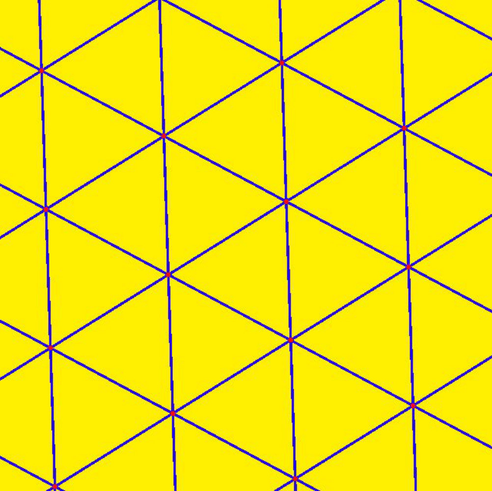 Figure 1
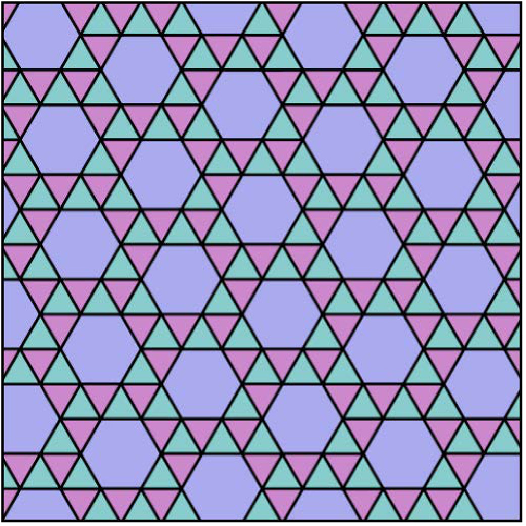 Figure 2
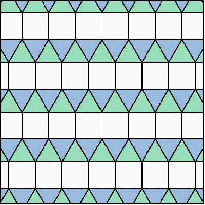 Figure 3
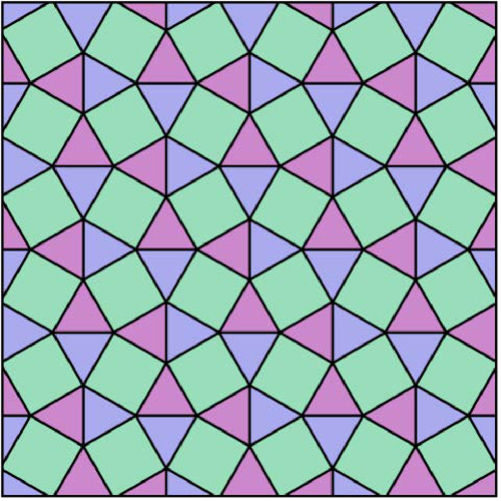 Figure 4
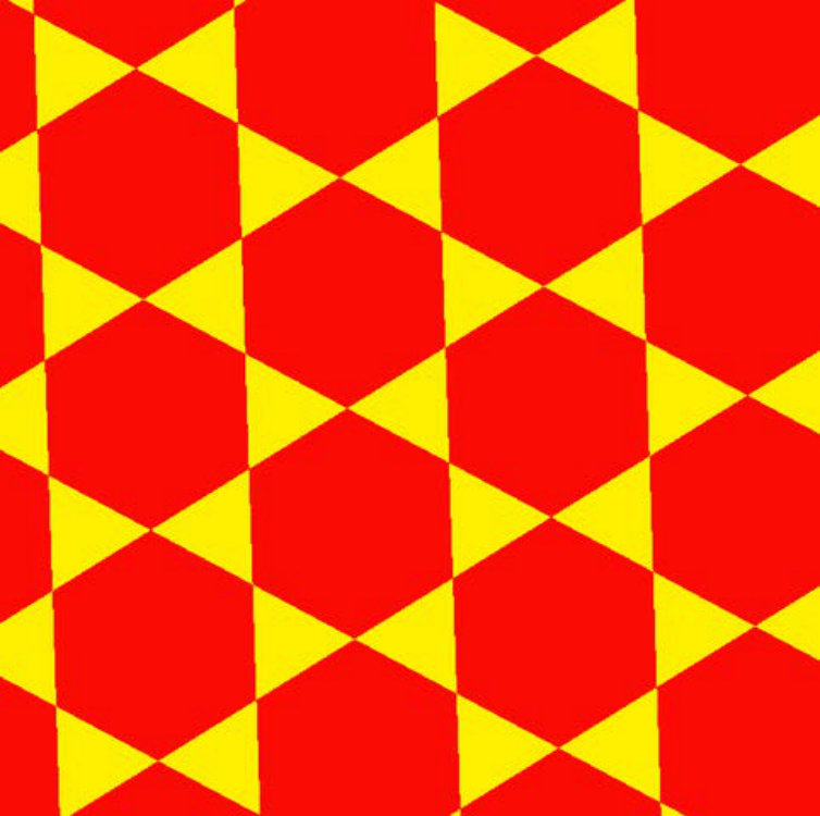 Figure 5
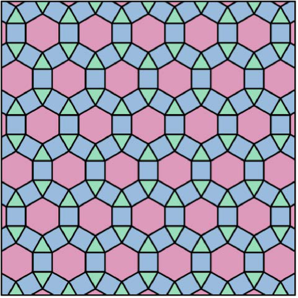 Figure 6
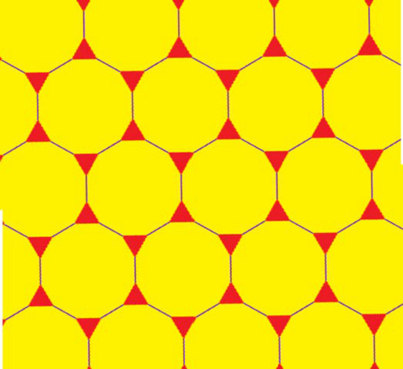 Figure 7
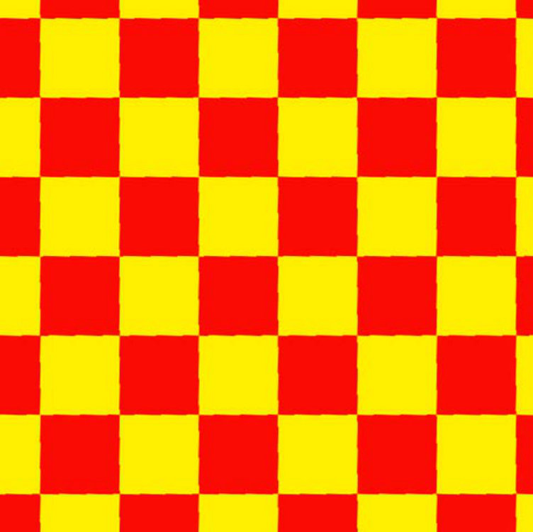 Figure 8
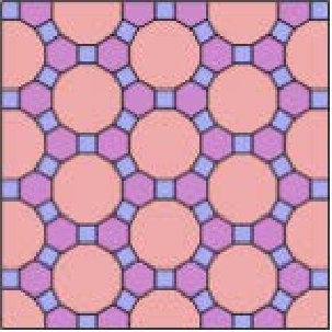 Figure 9
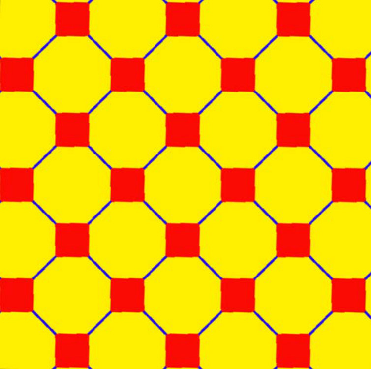 Figure 10
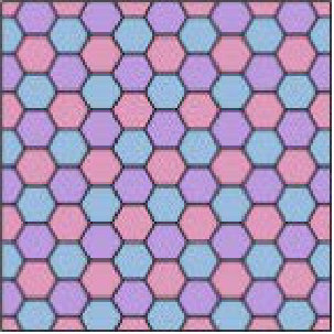 Figure 11
 Figure 12
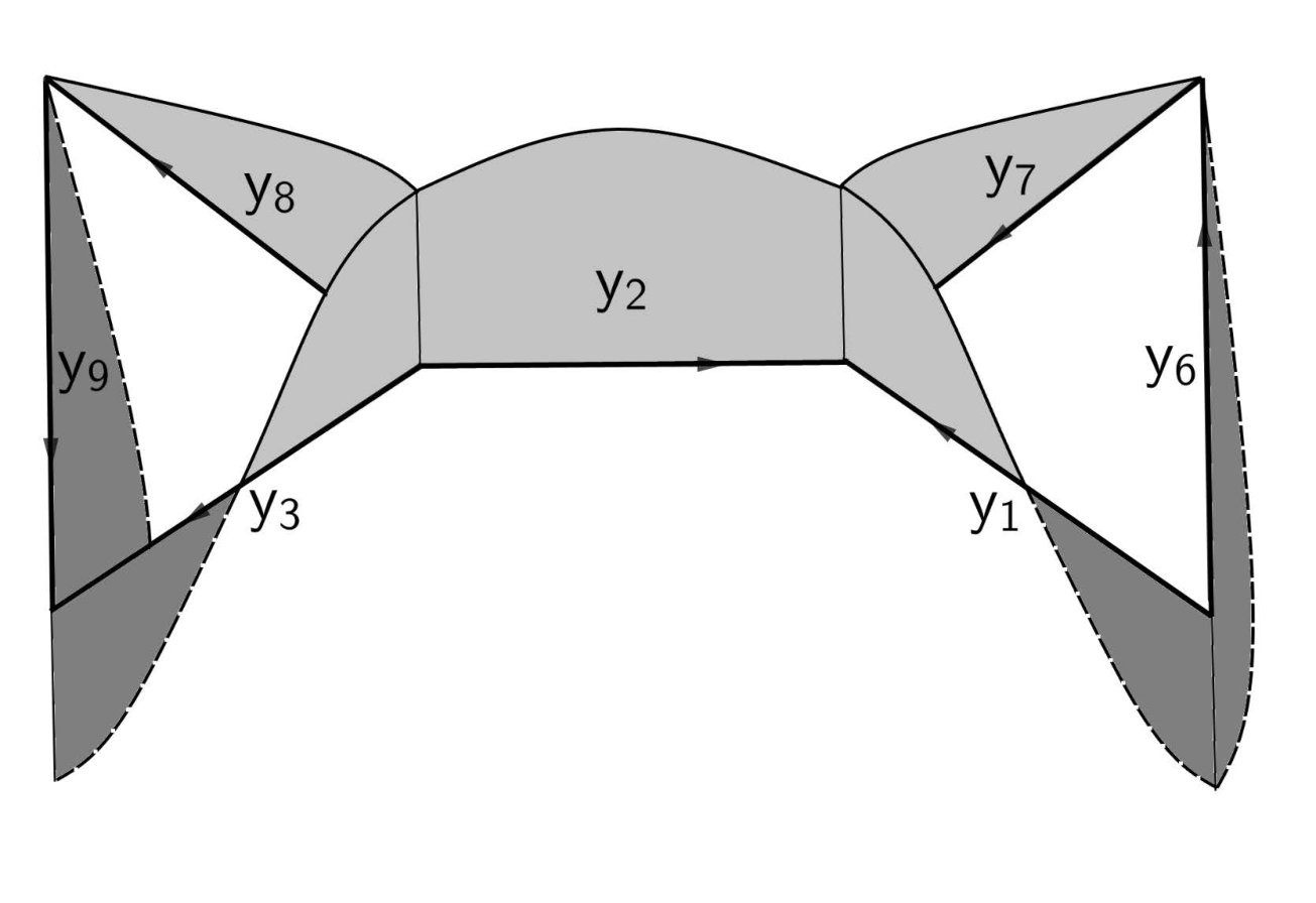 Figure 13
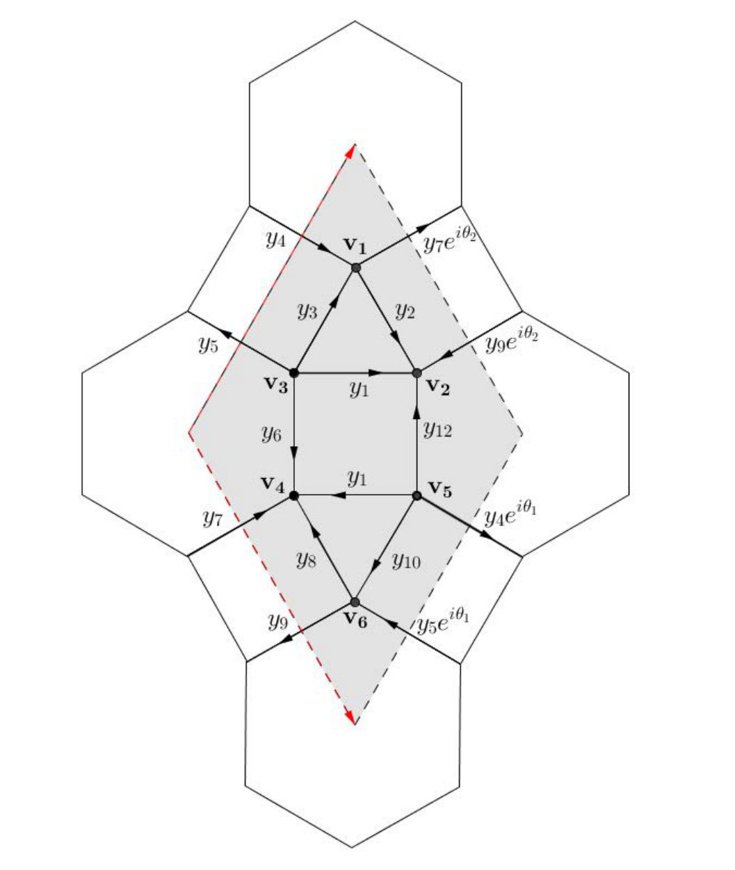 Figure 14
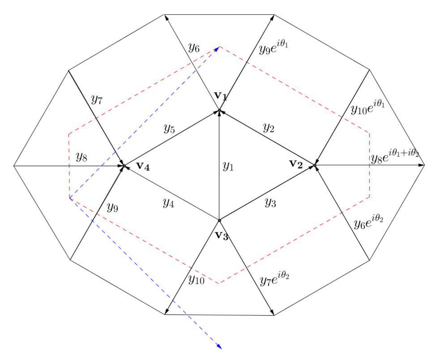 Figure 15
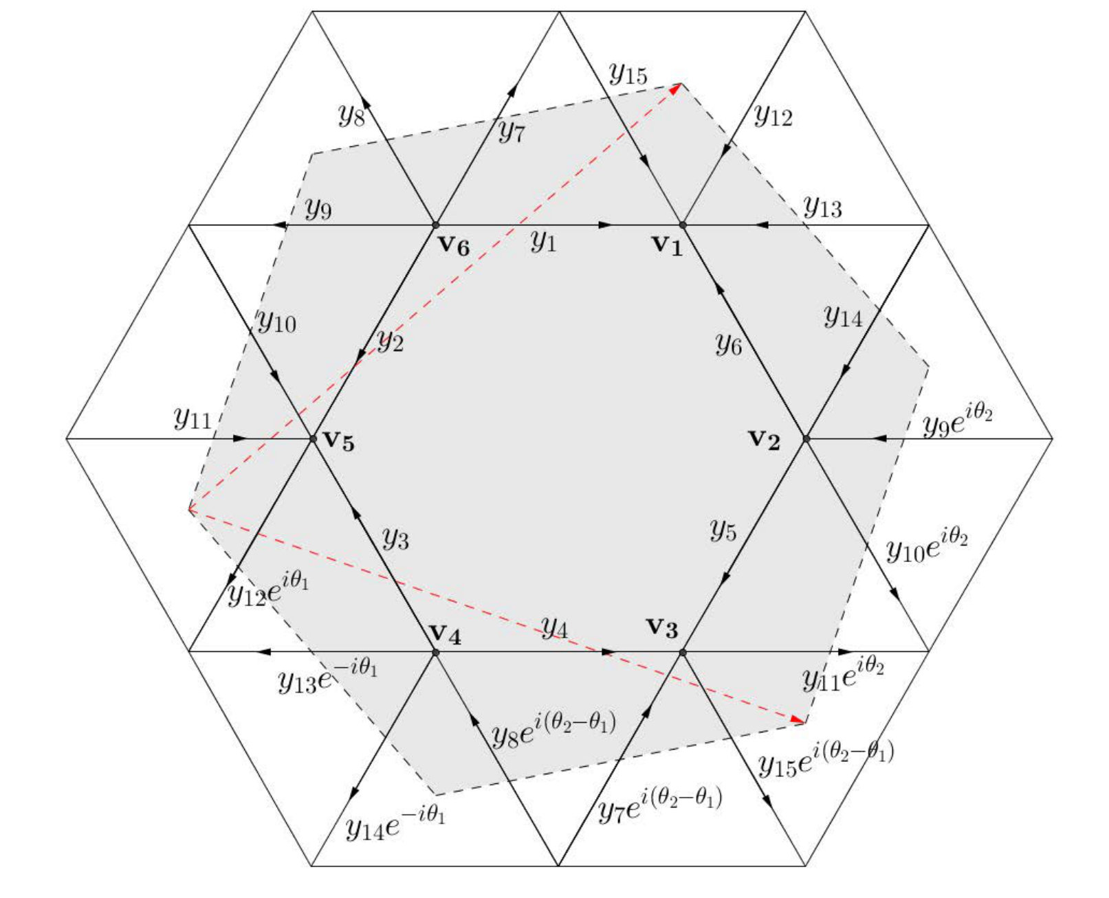 Figure 16
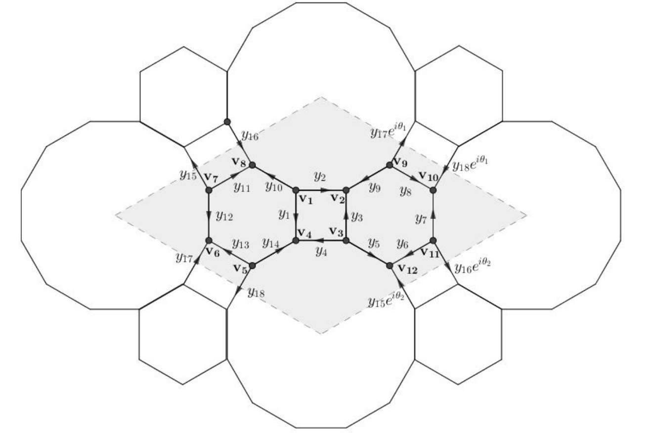 Figure 17
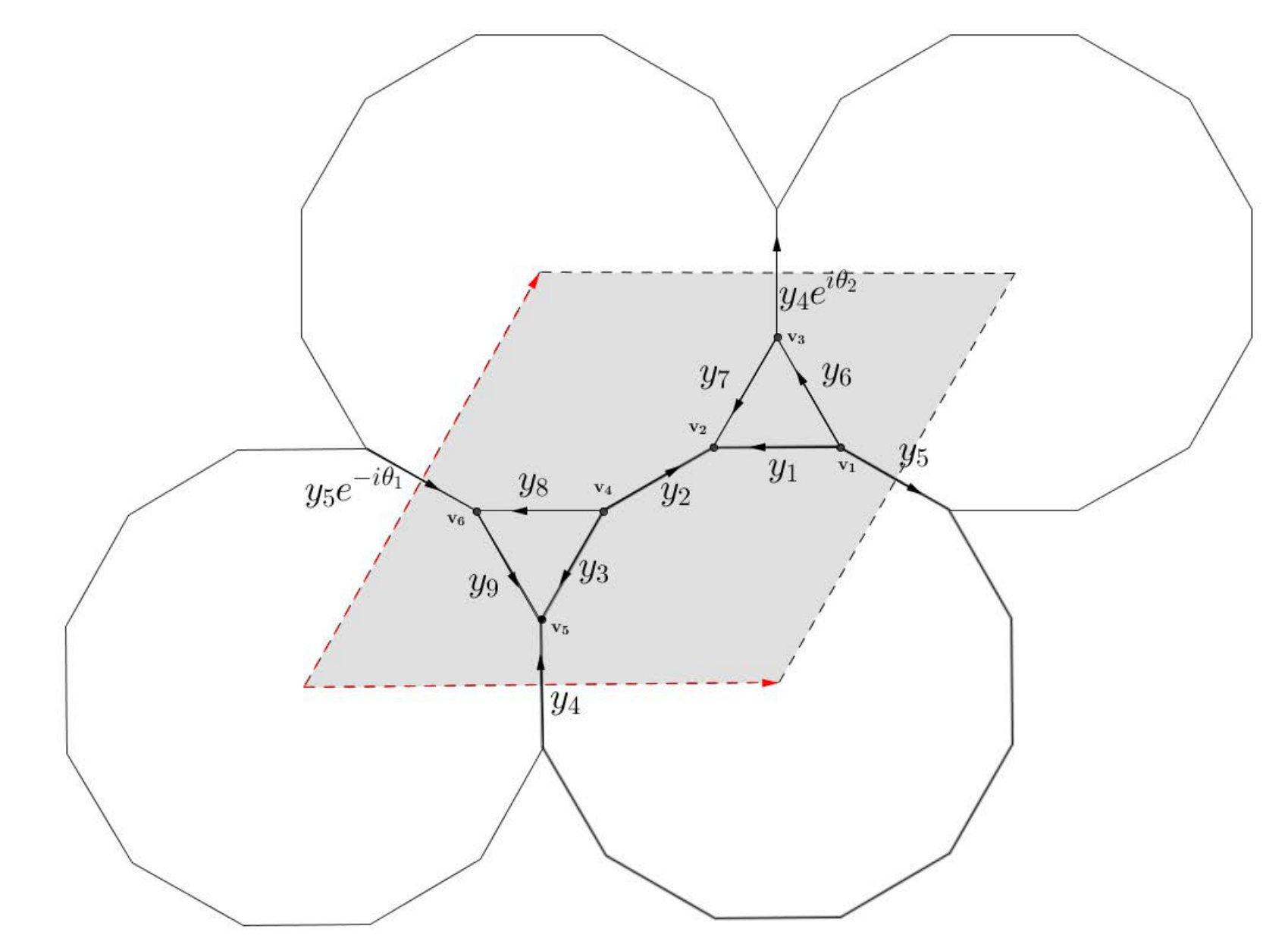 Figure 18
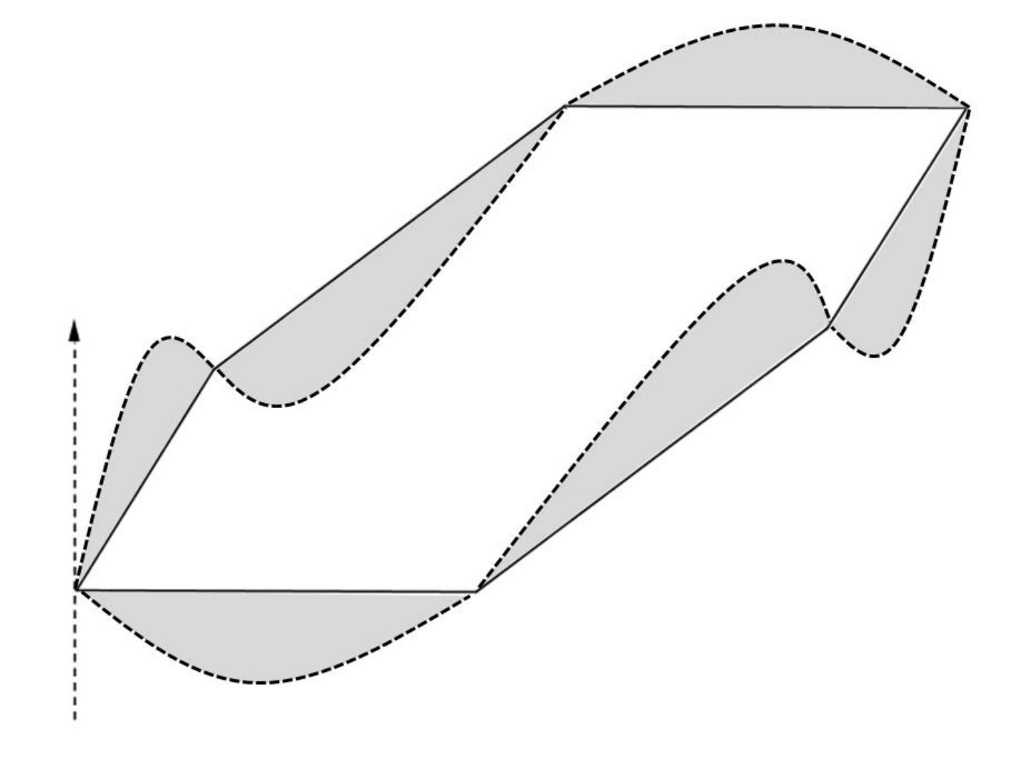 Figure 19
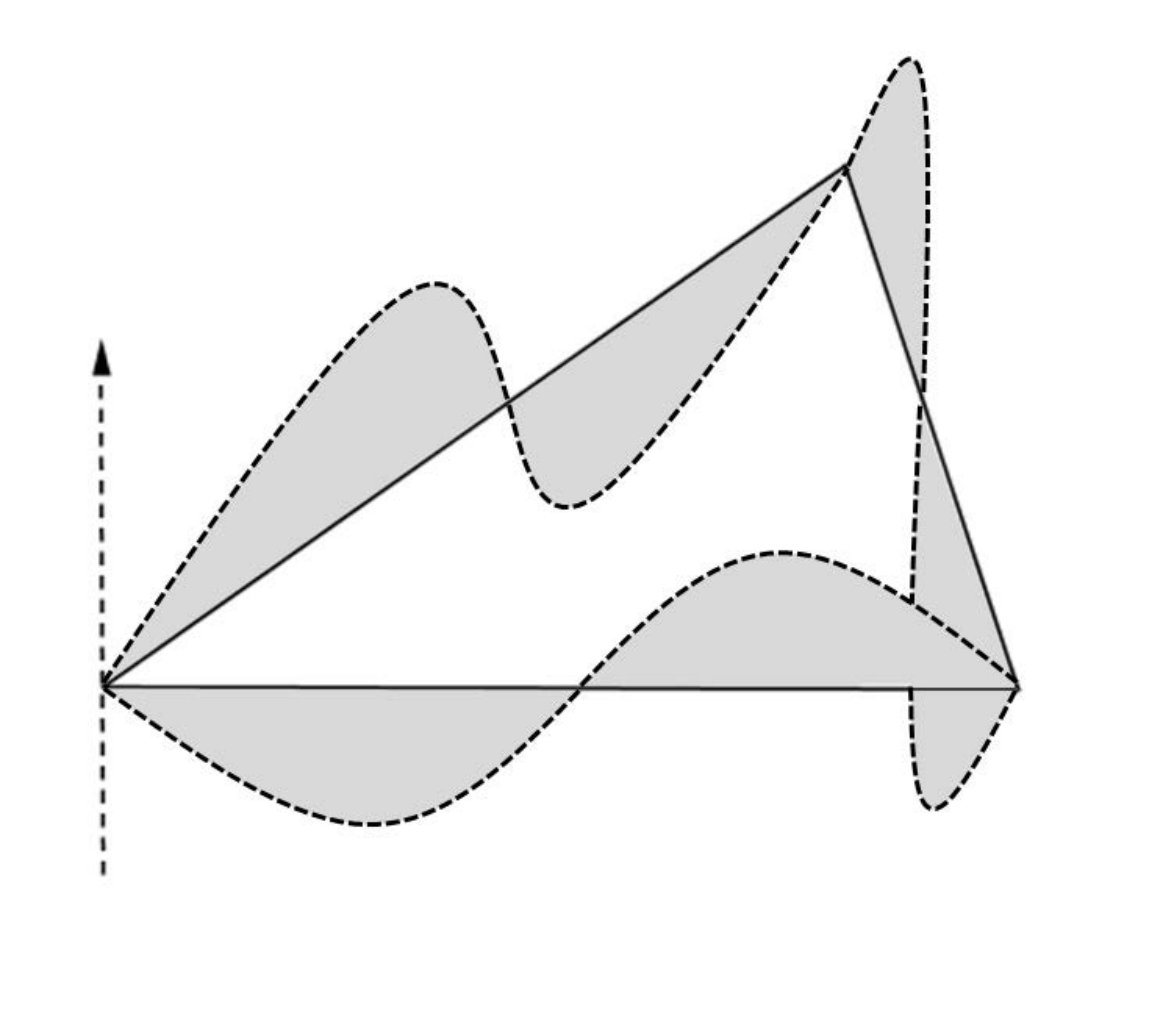 Figure 20
Peer Reviews
No public reviews on file for this paper yet. If you reviewed it on a platform where reviews are public (OpenReview, ICLR, NeurIPS, ICML), you can paste yours below so the community can read it here.
Videos
No videos yet. Explain this paper in a talk, walkthrough, or lecture? Add one.
Dispersion relations of periodic quantum graphs associated with Archimedean tilings (II)
Yu-Chen Luo
Department of Applied Mathematics, National Sun Yat-sen University, Kaohsiung, Taiwan 80424. Email: [email protected], [email protected]
Eduardo O. Jatulan
Department of Applied Mathematics, National Sun Yat-sen University, Kaohsiung, Taiwan 80424. Email: [email protected], [email protected]
Institute of Mathematical Sciences and Physics, University of the Philippines Los Baños, Philippines 4031. Email: [email protected]
Chun-Kong Law
Department of Applied Mathematics, National Sun Yat-sen University, Kaohsiung, Taiwan 80424. Email: [email protected], [email protected]
Abstract
We continue the work of a previous paper [12] to derive the dispersion relations of the periodic quantum graphs associated with the remaining 5 of the 11 Archimedean tilings, namely the truncated hexagonal tiling , rhombi-trihexagonal tiling , snub square tiling , snub trihexagonal tiling , and truncated trihexagonal tiling . The computation is done with the help of the symbolic software Mathematica. With these explicit dispersion relations, we perform more analysis on the spectra.
Keywords: characteristic functions, Floquet-Bloch theory, uniform tiling, absolutely continuous spectrum.
1 Introduction
On the plane, there are plenty of ways to form a tessellation with different patterns [7]. A tessellation is formed by regular polygons having the same edge length such that these regular polygons will fit around at each vertex and the pattern at every vertex is isomorphic, then it is called a uniform tiling. There are 11 types of uniform tilings, called Archimedean tilings in literature, as shown in Table 4. The periodic quantum graphs associated with these Archimedean tilings constitute good mathematical models for graphene [1, 10] and related allotropes [5]. In a previous paper [12], we employ the Floquet-Bloch theory, and the characteristic function method for quantum graphs to derive the dispersion relations of periodic quantum graphs associated with 4 kinds of Archimedean tilings. As the dispersion relations concerning with square tiling and hexagonal tiling have been found earlier [8, 10], there are 5 remaining Archimedean tilings: the truncated hexagonal tiling , rhombi-trihexagonal tiling , snub square tiling , snub trihexagonal tiling , and truncated trihexagonal tiling . The objective of this paper is to derive the dispersion relations associated with them, and explore some of the implications.
Given an infinite graph generated by an Archimedean tiling with identical edgelength , we let denote a Schrödinger operator on , i.e.,
[TABLE]
where is periodic on the tiling (explained below), and the domain consists of all admissible functions (union of functions for each edge ) on in the sense that
- (i)
for all ; 2. (ii)
; 3. (iii)
Neumann vertex conditions (or continuity-Kirchhoff conditions at vertices), i.e., for any vertex ,
[TABLE]
Here denotes the directional derivative along the edge from , is the set of edges adjacent to , and denotes the Sobolev norm of 2 distribution derivatives.
The defined operator is well known to be self-adjoint. As is also periodic, we may apply the Floquet-Bloch theory [2, 4, 14] in the study of its spectrum. Let be two linear independent vectors in . Define , and . For any set , we define to be an action on by a shift of . A compact set is said to be a fundamental domain if
[TABLE]
and for any different , is a finite set in . The potential function is said to be periodic if for all and all . Take the quasi-momentum in the Brillouin zone . Let be the Bloch Hamiltonian that acts on , and the dense domain consists of admissible functions which satisfy the Floquet-Bloch condition
[TABLE]
for all and all . Such functions are uniquely determined by their restrictions on the fundamental domain . Hence for fixed , the operator has purely discrete spectrum , where
[TABLE]
By an analogous argument as in [14, p.291], there is a unitary operator such that
[TABLE]
That is, for any , . Hence by [2, 14],
[TABLE]
Furthermore, it is known that singular continuous spectrum is absent in [9, Theorem 4.5.9]. These form the basis of our work.
If one can derive the dispersion relation, which relates the energy levels as a function of the quasimomentum . The spectrum of the operator will then be given by the set of roots (called Bloch variety or analytic variety) of the dispersion relation.
On the interval , we let and are the solutions of
[TABLE]
such that , . In particular,
[TABLE]
Furthermore it is well known that the Lagrange identity , and when is even, [13, p.8].
So for the periodic quantum graphs above, suppose the edges lie in a typical fundamental domain , while are the potential functions acting on these edges. Assume also that the potential functions ’s are identical and even. Then the dispersion relation can be derived using a characteristic function approach [11, 12].
Theorem 1.1** ([8, 10, 11, 12]).**
Assume that all the ’s are identical (denoted as ), and even. We also let . The dispersion relation of the periodic quantum graph associated with each Archimedean tiling is given by the following.
- (a)
For associated with square tiling,
[TABLE] 2. (b)
For associated with hexagonal tiling,
[TABLE] 3. (c)
For associated with triangular tiling,
[TABLE] 4. (d)
For associated with elongated triangular tiling,
[TABLE] 5. (e)
For associated with truncated square tiling,
[TABLE] 6. (f)
For associated with trihexagonal tiling,
[TABLE]
We note that there was a typo error in [12, Theorem 1.1(d)] about this relation. In fact, in [11, 12], the dispersion relations were derived without the restriction that ’s are identical and even, although the equations are more complicated. Also observe that all the above dispersion relations are of the form , where is a polynomial in , with . Note that the term determines the point spectrum , which is independent of the quasimomentum , while the terem determines the absolutely continuous spectrum in each case, as the quasimomentum varies in the Brillouin zone . So we obtained the following theorem in [12].
Theorem 1.2**.**
Assuming all are identical and even,
- (a)
. 2. (b)
. 3. (c)
.
In this paper, we shall study the 5 remaining Archimedean tilings. Here the dispersion relations are even more complicated. So we need to restrict ’s to be identical and even. Our method is still the characteristic function approach, putting all the information into a system of equations for the coefficients of the quasiperiodic solutions, and then evaluating the determinant of the resulting matrix. In all the cases, the matrices are large, even with our clever choice of fundamental domains. The sizes starts with , up to . So as in [12], we need to use the software Mathematica to help simplify the determinants of these big matrices. We first arrive at the following theorem.
Theorem 1.3**.**
Assume that all the ’s are identical (denoted as ), and even. We also let . The dispersion relation of the periodic quantum graph associated with each Archimedean tiling is given by the following.
- (a)
For associated with truncated hexagonal tiling (),
[TABLE] 2. (b)
For associated with snub square tiling (), with ,
[TABLE] 3. (c)
For associated with rhombi-trihexagonal tiling (),
[TABLE] 4. (d)
For associated with snub trihexagonal tiling (),
[TABLE] 5. (e)
For associated with truncated trihexagonal tiling (*),
[TABLE]
All the dispersion relations are of the form , where is a polynomial in . Thus the point spectrum of each periodic Schrödinger operator is determined by the term , while the absolutely continuous spectrum is determined by the part . As varies in the Brillouin zone, the range of can be derived through some tedious elementary algebra. The following is our second main theorem.
Theorem 1.4**.**
Assuming all are identical and even,
- (a)
. 2. (b)
. 3. (c)
. 4. (d)
. 5. (e)
.
There dispersion relation characterize the spectrum of each periodic Schrödinger operator in terms of the functions and , which are associated with the spectral problem on an interval. In this way, the spectral problem over a quantum graph is reduced to a spectral problem over an interval, which we are familiar with. In particular, if , then , and . Thus the spectrum of each periodic operator can be computed easily (cf. Corollary 7.3 below).
We remark that these periodic quantum graphs provide a good model for the wave functions of crystal lattices. This is the so-called quantum network model (QNM) [1]. For example, graphene is associated with hexagonal tiling, with an identical and even potential function , where is the distance between neighboring atoms. In fact under this model, several graphene-like materials, called carbon allotropes, are associated with periodic quantum graphs [3, 5]. Thus a study of the spectrum, which is the energy of wave functions, is important.
In sections 2 through 6, we shall derive the dispersion relations of the periodic Schrödinger operators acting on the 5 above-mentioned Archimedean tilings. We shall invoke the vertex conditions as well as the Floquet-Bloch conditions on the boundary of the fundamental domains. With the help of Mathematica, the determinants the large resulting matrices are evaluated and then simplified, generating the dispersion relations. In section 7, we shall further analyze the dispersion relations to evaluate the point spectrum (and generate some eigenfunctions), plus the range of for each periodic Schrödinger operator. In particular, we shall prove Theorem 1.4. Finally we shall have a section on concluding remarks, followed by two appendices.
2 Truncated hexagonal tiling
The truncated hexagonal tiling , denoted by , is a periodic graph on the plane determined by one triangle and two dodecagons around a vertex. Each edge has length . As shown in Fig.1, let be a parallelogram defined by two vectors and . Let . Obviously the entire graph is covered by the translations of , namely
[TABLE]
So is a fundamental domain of . Applying the continuity and Kirchhoff conditions coupled with Floquet-Bloch conditions, we obtain the following equations at:
[TABLE]
[TABLE]
Since , we can rewrite the above equations as a linear system of and , thus
[TABLE]
With and , the characteristic equation is given by the following determinant of a matrix, as given in Appendix A. This determinant seems to be too big. So we assume all potentials ’s are identical and even. Hence, , for any . Then we use Mathematica to compute and simplify according to the coefficients . It still look very wild. But after we apply the Lagrange identity , things looks simpler and some pattern comes up.
[TABLE]
If we assume to be even so that , the dispersion relation for the periodic quantum graph associated with truncated hexagonal tiling becomes
[TABLE]
3 Snub square tiling
The snub square tiling , denoted by , is a periodic graph on the plane determined by one triangle and one square, then two triangles and one more square around a vertex. Each edge has length . Let be an irregular hexagon as defined in Fig.2, with two translation vectors and . Let . Obviously the entire graph is covered by the translations of , namely
[TABLE]
So is a fundamental domain of . The continuity and Kirchhoff conditions together with the Floquet-Bloch conditions, yield the following equations at:
[TABLE]
Since , we can rewrite the above equations as a linear system of and , thus
[TABLE]
Let and . Then the characteristic function is given by the determinant of a matrix.
This determinant is quite big to handle. We simplify it by making the and to be the same as we did in the previous section. Then we use Mathematica to compute and simplify according to the coefficients . After the computation, it still looks complicated, involving around 300 terms. However, by the help of the Lagrange identity, , things looks a lot simpler and some pattern comes out. The characteristic function will be
[TABLE]
Now, if we assume to be even so that , the dispersion relation for the periodic quantum graph associated with snub square tiling will be
[TABLE]
Let and . This yields the dispersion relation in Theorem 1.3(b).
4 Rhombi-trihexagonal tiling
The rhombi-trihexagonal tiling , denoted by , is a periodic graph on the plane determined by one triangle, one square, one hexagon and another square around a vertex. Each edge has length . As shown in fig.3, let be a parallelogram defined by two vectors and . Let . Obviously the entire graph is covered by the translations of , namely
[TABLE]
This is a fundamental domain of . The continuity and Kirchhoff conditions coupled with Floquet-Bloch conditions yield:
[TABLE]
Since , we can rewrite the above equations as a linear system of and with and . Thus,
[TABLE]
Assume that the potential are identical, that is, and . So the characteristic equation is a determinant of matrix. With the help of Mathematica and Lagrange identity, , we evaluate the characteristics function as
[TABLE]
If we further assume that the the potential is even then , and it yields the dispersion relation in Theorem 1.3(c).
5 Snub trihexagonal tiling
The snub trihexagonal tiling , denoted by , is a periodic graph on the plane determined by three triangles and one hexagon around a vertex. Each edge has length . Let be a regular hexagon as defined in Fig.4, with two translation vectors and . Let is a fundamental domain of .
We apply the continuity and Kirchhoff conditions coupled with Floquet-Bloch conditions to obtain:
[TABLE]
[TABLE]
Since , we can rewrite the above equations as a linear system of and with and . Thus,
[TABLE]
Next we assume that the potential are identical so that and . The characteristic equation is thus a determinant of matrix. With the help of Mathematica and Lagrange identity, we evaluate the characteristic function as
[TABLE]
If the potential is even then . Therefore Theorem 1.3(d) is valid.
6 Truncated trihexagonal tiling
The truncated trihexagonal tiling , denoted by , is a periodic graph on the plane determined by one square, one hexagon and one dodecagon around a vertex. Each edge has length . As shown in fig.4, let be a parallelogram defined by two vectors and . Let is a fundamental domain of .
Applying the continuity and Kirchhoff conditions coupled with Floquet-Bloch conditions, we obtain:
[TABLE]
Since , we rewrite the above equations as a linear system of and with and . Thus,
[TABLE]
Then we assume that the potential are identical. In this way, the characteristic equation is the determinant of a matrix. The characteristics function, after evaluation of the determinant, is given by
[TABLE]
After simiplification,
[TABLE]
In case is even then , and Theorem 1.3(e) holds.
7 More analysis on the spectrum
In this section, we study the spectra of these periodic quantum graphs in more detail. That is, we try to understand the behavior of the point spectrum and the absolutely continuous spectrum .
Theorem 7.1**.**
Assuming all ’s are identical and even we have the following
- a.
Let be the spectrum of the periodic quantum graph associated with truncated hexagonal tiling. Then
[TABLE] 2. b.
The point spectrum of the periodic quantum graph associated with snub square tiling (), rhombi-trihexagonal tiling (), snub trihexagonal tiling (), and truncated trihexagonal tiling () coincide and is given by the set
[TABLE]
The above theorem follows immediately from the fact that point spectrum contains exactly those which do not vary with .
Clearly the Bloch variety for the factor generates the Dirichlet-Dirichlet eigenfunctions along any polygon (triangle, rectangle, hexagonal, or dodecagon), and extended by zero to the whole graph, as shown in Fig.6. Truncated hexagonal tiling is interesting in that its dispersion relation has two more factors . The Bloch variety associated with the factor generates an eigenfunction with support on the six triangle around the edges of a dodecagon, and be extended to the whole graph by zero (cf. Fig.1 and Fig.7a). In particular, let such that . Then
[TABLE]
The pattern goes round the dodecagon and it is easy to see that the Neumann conditions are satisfied at the vertices.
For the case , we let so that . Define
[TABLE]
It is easy to that is a solution that satisfies , so the the Neumann conditions are met (cf. Fig.1 and Fig.7b).
Hence every element of point spectra has infinitely many eigenfunctions. We conjecture that the functions discussed above are all the eigenfunctions, but we cannot prove it. For the absolutely continuous spectrum for each Archimedean tiling, we have the following theorem.
Theorem 7.2**.**
Assuming all ’s are identical and even, we have the following
- a.
. 2. b.
. 3. c.
. 4. d.
. 5. e
.
Proof.
- (a)
Let . From Theorem 1.3(a), if and only if
[TABLE]
or equivalently,
[TABLE]
where . Recall the trigonometric identity (see [10] and [12, Eq.(1.6)])
[TABLE]
which implies that for any . Now the function is a quartic polynomial with with critical points at . Its global minimum points are located at and . It also has a local maximum point at , and approaches to as . Also on the intervals , and , while is a constant function ranging from to [math]. It is thus obvious that the dispersion relation (7.5) is satisfied iff , whence . 2. (b)
Let , and , . From 1.3(b), we have
[TABLE]
If , this is equivalent to , with
[TABLE]
It is easy to see that is a quartic polynomial with two global minimum points at , one local maximum point at , and approaches to as . Also
[TABLE]
It is easy to show that the graph of lies below that of and is tangent at the points . On the other hand, the graph of intersects that of at the points and , and is above the graph of on this interval . Since is continuous in , we conclude that if , then . Now, let . Then (7.7) yields that for all ,
[TABLE]
because the constant term is . Also, if for then (7.7) yields that for all ,
[TABLE]
because the constant term is . Therefore, if and only if . 3. (c)
As before, let . From Theorem 1.3(c), the absolutely continuous spectrum is characterized by
[TABLE]
with
and because by ((a)),
[TABLE]
Let us first look at the special case when , and and . Then
[TABLE]
Thus the above dispersion relation becomes
[TABLE]
for . Here is an even polynomial with global minimum points at , two local maximum points at , and one local minimum point at . Also approaches to as . The right hand side is in general a cubic polynomial. We shall study three cases:
[TABLE]
The graph of is a line that intersects that of at . Also on . The graph of intersects that of at . Furthermore on , while on . Thus by continuity of , if lies in , then (7.9) is valid for some . On the other hand, and have the same values at ; and on while on . Comparing with the properties of , we conclude that for , there exists such that (7.9) is valid. Therefore .
We shall see that this is indeed the entire range of , for any . Suppose for then (7.8) reduces to
[TABLE]
because all coefficients are nonnegative (Please refer to Appendix B for detailed argument).
Also, if for some , then (7.8) implies
[TABLE]
because all coefficients are nonnegative (cf. Appendix B for detail). Therefore, if and only if . 4. (d)
Let be as defined above. By the trigonometric identity ((a)), the dispersion relation given by Theorem 1.3(d) is simplified to
[TABLE]
Let . The absolutely continuous spectrum is characterized by
[TABLE]
Now let , . Then (7.10) becomes
[TABLE]
Let denote the polynomial on the right hand side. We study and in more detail. Since
[TABLE]
then on and on . Also,
[TABLE]
Hence on and on . Since is continuous in , it follows that (7.10) is valid for some when .
Now, for the interval , we let for some . Then
Let . Then
[TABLE]
To show that (7.10) is valid for some when , since for all , it suffices to show that for any we have for some . Now, for any consider . One can easily check that . Substituting we have
[TABLE]
The above inequality is due to the fact that has 0 as its maximum value in .
Now, suppose (), then the left hand side of (7.10) yields
[TABLE]
Also, if for some , then
[TABLE]
Therefore, . 5. (e)
Let , and
Then from Theorem 1.3(e) and the trigonometric identity ((a)), the absolutely continuous spectrum is characterized by
[TABLE]
We want to show that this is valid if and only if , or equivalently . Now let , . Then
[TABLE]
and (7.12) becomes , where
[TABLE]
We study two special ’s, namely
[TABLE]
It is routine to see that
[TABLE]
Hence for all . By continuity, is a subset of the characterization domain.
Next, we show that is also a subset. Let . Then we have
[TABLE]
Since , for all , it suffices to show that for any we have for some . Now, for , let . It is easy to check that . Substituting this we get
[TABLE]
The above inequality is due to the fact that has 0 as its maximum value in .
Now let , then (7.12) will be
[TABLE]
(cf. Appendix B). If for some , then (7.12) becomes
,
(cf. Appendix B). Also, if for , then we have
[TABLE]
(cf. Appendix B). Therefore, we conclude that if and only if .
∎
In the case , then . Hence we have the following corollary.
Corollary 7.3**.**
When , we have
- (a)
,
where , . 2. (b)
, where . 3. (c)
, where . 4. (d)
, where . 5. (e)
, where
8 Concluding remarks
As a summary, we have derived the dispersion relations for the periodic quantum graphs associated with all the 11 Archimedean tilings. We showed that they are all of the form for some , and is a polynomial of . The spectrum is exactly Bloch variety. Here the point spectrum is defined by ; while the absolutely continuous spectrum is defined by , For the 5 Archimedean tilings discussed in this paper, we can find many eigenfunctions, each of which has infinite multiplicity. Some nontrivial eigenfunctions for trihexagonal tiling and truncated hexagonal tiling are also found. The spectra are all of a band and gap structure. Also their absolutely continuous spectra satisfy where . Moreover the absolutely continuous spectra corresponding to each of the square tiling, hexagonal tiling, truncated square tiling and truncated trihexagonal tiling satisfies . As the function behaves asymptotically like , as , we know that the spectral gaps tends to zero.
We also remark that for , is always a solution for , for all the 11 Archimedean tilings. We also perform numerical checkup for specific values of to check those dispersion relations derived using symbolic software. Thus we are confident that the dispersion relations in this paper are correct. Thus our method is an efficient and effective one for any complicated periodic quantum graphs.
Recently, Fefferman and Weinstein [6] embarked on a systematic study of the case of hexagonal tiling (also called honeycomb lattice). Based on a PDE approach, assuming that the wave functions acts on the whole hexagon, they showed that there exists infinitely many Dirac points in the spectrum. In our case, Dirac points are the points where with , and the relationship is asymptotically a cone (called Dirac cone) [3]. As explained in [6, 3], the existence of Dirac points accounts for the electronic properties of graphene and related crystal lattices. It is desirable to study when there exist infinitely many Dirac points, not only for hexagonal tiling, but also for the other 10 Archimedean tilings. We shall pursue on this issue later.
Acknowledgements
We thank Min-Jei Huang, Ka-Sing Lau, Vyacheslav Pivovarchik and Ming-Hsiung Tsai for stimulating discussions. We also thank the anonymous referees for helpful comments. The authors are partially supported by Ministry of Science and Technology, Taiwan, under contract number MOST105-2115-M-110-004.
Appendix A Characteristic matrix for truncated hexagonal tiling
[TABLE]
Appendix B Some inequalities in the proof of Theorem 7.2
This section gives the details of some tedious arguments in the proof of Theorem 7.2(c),(d) and (e)
- (c)
We claim that . for any and . Now, let and , then we have the following:
[TABLE]
So we have
[TABLE]
The second part is to show that for . Let
[TABLE] 2. d.
Here we want to show that for any and . With the same change of variable as above,
[TABLE]
The second part is to investigate . Consider ,
[TABLE]
Knowing that when , we design a factorization to solve the problem.
[TABLE]
Therefore is nonnegative. 3. (e)
Let . The first part is to study . Observe that
[TABLE]
So is nonnegative. The second part is to show that . Here
[TABLE]
Finally we want to show that when , for all
With the same substitution as above for and , we have
[TABLE]
Hence, the problem is equivalent to showing that for a fixed then for all .
We shall use calculus to deal with it. To compute for the critical points of in the interior of ,
[TABLE]
If then . Substituting this to (2.13) we get
[TABLE]
So from (2.15), it is clear that the critical points of are the point , , and . However, the only critical point inside is at the points . Moreover, , for all .
Now, we focus on the boundary of . Along :
and
. Thus, has no critical points.
Along :
and
. Thus, has no critical points.
Along :
and
. It is easy to see that the critical points of are the points and . One can show that , for all . Thus, is the only critical number and , for all .
Along :
and
. It is easy to see that the critical points of are the points and . One can show that . Thus, is the only critical number and .
Also, , and . Therefore, the claim holds.
The reference list from the paper itself. Each links out to its DOI / PubMed record.
- 1[1] C. Amovilli, F.E. Leys, and N.H. March, Electronic energy spectrum of two-Dimensional solids and a chain of C atoms from a quantum network model, J. Math. Chem. , 36 (2004), 93-112.
- 2[2] G. Berkolaiko and P. Kuchment, Introduction to Quantum Graphs , Amer. Math. Soc., Providence, 2012.
- 3[3] N.T. Do and P. Kuchment, Quantum graph spectra of a graphyne structure, Math. Quantum Nano Tech. , 2 (2013) 107-123.
- 4[4] M. Eastham, The Spectral Theory of Periodic Differential Equations , Scottish Academic Press, Edinburgh and London, 1973.
- 5[5] A. Enyanshin and A. Ivanovskii, Graphene alloptropes: stability, structural and electronic properties from DF-TB calculations, Phys. Status Solidi (b) , 248 (2011) 1879-1883.
- 6[6] C.L. Fefferman and M.I. Weinstein, Honeycomb lattice potentials and Dirac points, J. Amer. Math. Soc. 25 , (2012) 1169-1220.
- 7[7] B. Grünbaum and G. Shephard, Tilings and Patterns , W. H. Freeman and Company, New York, 1987.
- 8[8] E. Korotyaev and I. Lobanov, Schrödinger operators on zigzag nanotubes, Ann. Henri Poincaré , 8 (2007), 1151-1176.