Relaxing The Hamilton Jacobi Bellman Equation To Construct Inner And Outer Bounds On Reachable Sets
Morgan Jones, Matthew M. Peet

TL;DR
This paper introduces a method to approximate both inner and outer bounds of reachable sets for polynomial systems by relaxing the Hamilton-Jacobi-Bellman equation, using polynomial bounds on the value function.
Contribution
It presents a novel approach to construct provable bounds on reachable sets via polynomial sub- and super-value functions solving a relaxed HJB PDE.
Findings
Polynomial bounds effectively approximate reachable sets.
Inner and outer bounds have negligible Hausdorff distance at low polynomial degree.
Method applicable to systems with polynomial dynamics and semialgebraic constraints.
Abstract
We consider the problem of overbounding and underbounding both the backward and forward reachable set for a given polynomial vector field, nonlinear in both state and input, with a given semialgebriac set of initial conditions and with inputs constrained pointwise to lie in a semialgebraic set. Specifically, we represent the forward reachable set using the value function which gives the optimal cost to go of an optimal control problems and if smooth satisfies the Hamilton-Jacobi- Bellman PDE. We then show that there exist polynomial upper and lower bounds to this value function and furthermore, these polynomial sub-value and super-value functions provide provable upper and lower bounds to the forward reachable set. Finally, by minimizing the distance between these sub-value and super-value functions in the L1-norm, we are able to construct inner and outer bounds for the reachable set…
Click any figure to enlarge with its caption.
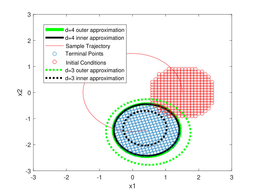 Figure 1
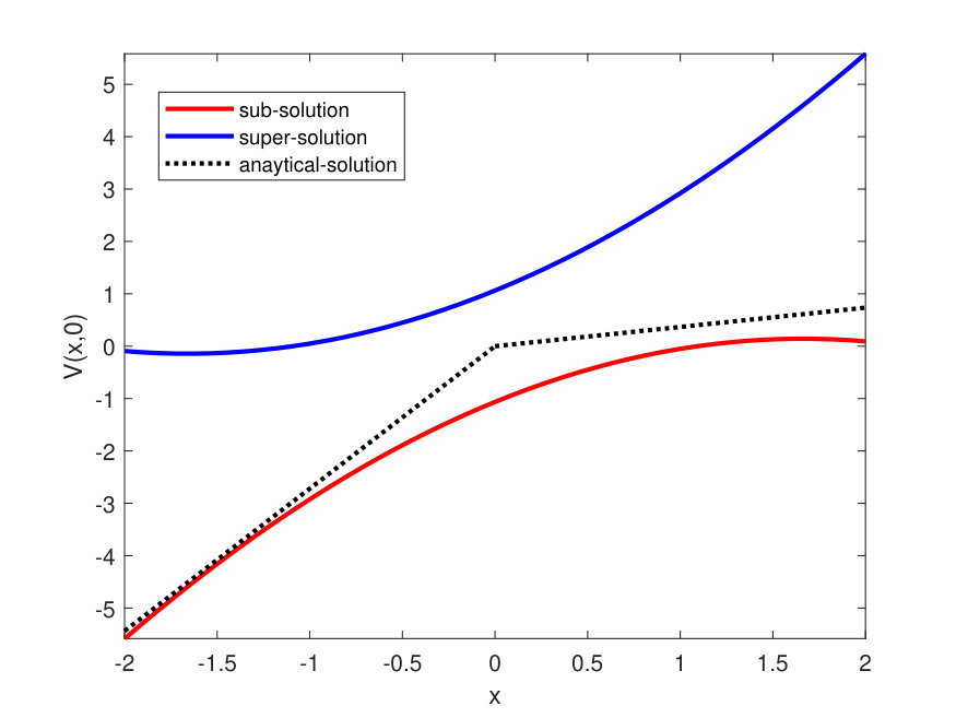 Figure 2
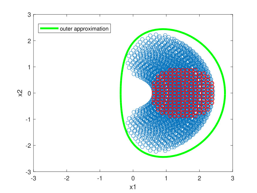 Figure 3
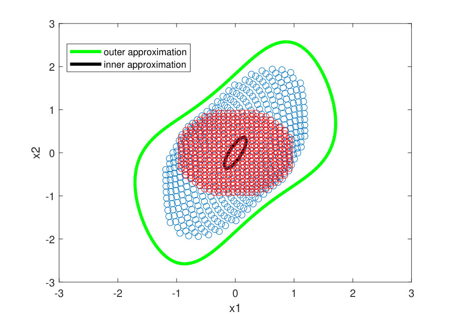 Figure 4
Peer Reviews
No public reviews on file for this paper yet. If you reviewed it on a platform where reviews are public (OpenReview, ICLR, NeurIPS, ICML), you can paste yours below so the community can read it here.
Videos
No videos yet. Explain this paper in a talk, walkthrough, or lecture? Add one.
Relaxing The Hamilton Jacobi Bellman Equation To Construct Inner And Outer Bounds On Reachable Sets
Morgan Jones, Matthew M. Peet M. Jones is with the School for the Engineering of Matter, Transport and Energy, Arizona State University, Tempe, AZ, 85298 USA. e-mail: [email protected] M. Peet is with the School for the Engineering of Matter, Transport and Energy, Arizona State University, Tempe, AZ, 85298 USA. e-mail: [email protected]
Abstract
We consider the problem of overbounding and underbounding both the backward and forward reachable set for a given polynomial vector field, nonlinear in both state and input, with a given semialgebriac set of initial conditions and with inputs constrained pointwise to lie in a semialgebraic set. Specifically, we represent the forward reachable set using the “value function” which gives the optimal cost to go of an optimal control problems and if smooth satisfies the Hamilton-Jacobi-Bellman PDE. We then show that there exist polynomial upper and lower bounds to this value function and furthermore, these polynomial “sub-value” and “super-value” functions provide provable upper and lower bounds to the forward reachable set. Finally, by minimizing the distance between these “sub-value” and “super-value” functions in the -norm, we are able to construct inner and outer bounds for the reachable set and show numerically on several examples that for relatively small degree, the Hausdorff distance between these bounds is negligible.
I Introduction
The reachable set of an ODE is the set of coordinates that can be reached by the solution map, defined in Assumption 1, at some fixed time and starting in some set of initial conditions. The computation of reachable sets is important for certifying solution maps remain in “safety regions”; regions of the state space that are deemed to have low risks of system failure. Historic examples of solution maps transitioning outside “safe regions” include: two of the four reaction wheels on the Kepler Space telescope failing, analyzed in [1]; and the disturbing lateral vibrations of the Millennium footbridge over the River Thames in London on opening day, analyzed in [2] and [3].
In this paper we show the reachable set of an ODE, subject to pointwise bounded inputs, is the sublevel set of the “value function” (optimal cost to go function) associated with a one player optimal control problem. This result can be thought of as the analogous result to [4]; where it was shown the reachable set of an ODE, subjected to two sets of adversarially opposed input parameters, is the sublevel set of the “value function” associated with a two player optimal control problem.
It is known that if the “value function” of a one player optimal control problem is smooth then it satisfies the Hamilton Jacobi Bellman (HJB) Partial Differential Equation (PDE) [5]. In this paper we show that relaxing the HJB PDE to a dissipation inequality allows for the construction of upper and lower bounds of the ”value function”; we call super-value and sub-value functions respectively. We futhermore give sufficient conditions for the existence of polynomial super-value and sub-value functions. Moreover, it is shown that the sublevel set of sub-value and super-value functions construct provable upper and under bounds of reachable sets respectively.
The HJB PDE may not always have a solution in the classical sense. A generalized solution concept, called the viscosity solution, was developed in [6]. Discretization methods, such as those in [7] [8], are typically used to approximate the viscosity solution. However, such methods cannot guarantee that the approximate viscosity solution is an upper or lower bound to the true ”value function”. Alternatively, we propose a Sum-of-Squares (SOS) optimization problem that is solved by the polynomial sub-value and super-value functions with minimum distance.
Our approach to finding sub- and super-solutions to the HJB PDE is similar to [9] and [10]. In [9] SOS was used to find a sub-value function for optimal control problems with discrete-time dynamics; whereas we consider continuous-time dynamics. In [10] SOS was used to find sub-value and super-value functions for optimal control problems with quadratic costs and continuous-time synamics governed by ODE’s affine in the input variable. Our approach allows us to construct sub-value and super-value functions for more general optimal control problems with polynomial costs and continuous time varying processes governed by ODE’s nonlinear in the input variable. Moreover, we give sufficient conditions on the existence of polynomial sub-value and super-value functions and show how these functions can be used for reachable set estimation.
We numerically demonstrate that solving our proposed SOS optimization problem can give tight approximations of reachable sets. Unlike alternative approaches to reachable set analysis, [4] [11] [12], our reachable set approximations can be proved to overbound or underbound the reachable set.
An alternative approach to reachable set approximation is found in [13] [14] [15] [16] where dissipation like inequalities are solved using SOS programing to find a function whose sublevel set contains the reachable set. It is shown in this paper such dissipation inequalities are actually relaxations of the HJB PDE and thus solved by sub-value functions. In this context, our sufficient conditions for the existence of polynomial sub-value functions for optimal control problems can be viewed as feasibility conditions for the SOS optimization problems found [13] [14] [15] [16].
The paper is organized as follows. Background material on ODE’s is given in Section III. In Section IV optimal control theory is presented. In Section V we construct an optimal control problem with value function that can characterize the reachable set exactly. In Section VI we show how relaxing the HJB PDE allows us to derive dissipation inequalities that are solved by sub-value and super-vale functions. In Section VII an SOS optimization is proposed that minimizes the norm of the distance between the sub-value and super-value function. The conclusion is given in Section VIII.
II Notation
We denote a ball with radius centered at the origin by . For we denote . For short hand we denote the partial derivative for . Let be the Banach space of scalar continuous functions with domain . For we define the norms and . We denote the set of differentiable functions by . For we denote and . For and we denote to be the vector of monomial basis in -dimensions with maximum degree . We denote the space of scalar valued polynomials with degree at most by . We say is Sum-of-Squares (SOS) if there exists such that . We denote to be the set of SOS polynomials.
III Background: Differential Equations
We consider nonlinear Ordinary Differential Equations (ODE’s) of the form
[TABLE]
where ; is the input; and and are compact sets representing constraints on the inputs and initial conditions.
To define the solution map we define the set of pointwise-admissible input signals as
[TABLE]
For a given set of admissible inputs, we constrain , in the following definition, to admit a continuously-differentiable solution map.
Definition 1** (Constraint on Admissibility of )**
For given we say if
* for all .* 2. 2.
For any , there exists a function , where for any we have for all , and
[TABLE]
for all , and . 3. 3.
The function that satisfies (2) is unique.
Since for each the associated function that satisfies (2) is unique we will denote this function by throughout the paper.
Lemma 1
Let be a compact set, and .
- (A)
For define , then
[TABLE] 2. (B)
For and define , then
[TABLE]
Proof:
Proving (3) in Statement (A): As we have for all , , and
[TABLE]
Now, letting , for , , and the following holds
[TABLE]
where to get the second equality we use , so ; to get the third equality (5) was used; to get the fourth equality the substitution was again applied, noting . Moreover, as , by (5), it follows satisfies (2) and therefore, due to the uniqueness of , (3) must follow.
Proving (4) in Statement (B): For fixed let us consider the following function
[TABLE]
We prove (4) by showing satisfies (2) and using the uniqueness properties of . Firstly it is clear , and satisfies (2) for all , and . Now for all , and
[TABLE]
where the second equality follows from using so ; the third equality follows by (2); the fourth equality follows from applying again; the fifth equality follows as .
Thus by the uniqueness of it follows , therefore showing (4).
∎
For a given , and , we next define the forward reachable set as follows.
Definition 2
For , , and , let
[TABLE]
In following sections, is of the form either or .
IV Finite Time Optimal Control Problems
An optimal control problem with finite time horizon is a tuple where is the running cost; is the terminal cost; ; is the set of initial conditions; is a compact input set; and is the final time. For each optimal control problem we can next define the value function that intuitively describes the optimal ”cost to go”.
Definition 3
For given ; ; ; ; ; we say is a value function of the tuple if for , where , the following holds
[TABLE]
A sufficient condition for to be a value function for the tuple is for to satisfy the Hamilton Jacobi Bellman (HJB) PDE.
Proposition 1
For given , , , , , , suppose there exists a differentiable function such that the following holds for
[TABLE]
*Then is the value function of the optimal control problem . *
Proof:
Follows by Proposition 3.2.1 from [5] where the domain of the value function is restricted to . ∎
Definition 4
We say the function is a sub-value function to the finite time horizon optimal control problem if we have
[TABLE]
where is the value function of . Moreover if instead satisfies
[TABLE]
we say is a super-value function to .
V How Sublevel Sets Of Value Functions Can Describe Reachable Sets
In this section we construct a finite time horizon optimal control problem with associate value function whose sublevel sets can construct the reachable set of a system. We then show how the sublevel sets of the sub-value and super-value functions over- and under-bound the reachable set.
Analogous to Definition 2 we now define the backward reachable set and show how it is related to the forward reachable set in Lemma 2.
Definition 5
For , , and , let
[TABLE]
In the next Lemma we give a relationship between the backward reachable set and forward reachable set. This relationship shows finding the set is equivalent to finding the set . Therefore for the rest of this paper we concentrate on developing methods to bound the backward reachable set. However, for numerical implementation we will change the sign of the vector field to allow for the calculation of forward reachable set bounds.
Lemma 2
*Suppose , is such that , and . Then *
Proof:
We first show . For there exists and such that
[TABLE]
If we denote and , it now follows
[TABLE]
where the first equality follows by (8), the second equality by (3), and the third equality follows by (4). Thus we deduce from (9) .
We next show . For there exists and such that
[TABLE]
Let us denote , then it now follows
[TABLE]
where the first equality follows (3), the second equality by (10), and the third equality by (4). Thus we deduce . ∎
Theorem 1
Given , and , let and be such that . Now suppose is a value function for , then
[TABLE]
Proof:
As is a value function to it follows for all and
[TABLE]
For there exists and such that . Thus it follows
[TABLE]
where the first equality follows as so (12) holds. Therefore . Hence .
Now suppose . Then if , let . It follows
[TABLE]
where the third equality follows because so (12) holds. Hence . Therefore . Thus . ∎
We next show how sub-value and super-value functions, defined in Definition 4, can can outer bound and inner bound reachable sets.
Lemma 3
Given , and , let and be such that . Suppose and are sub-value and super-value functions to the optimal control problem . Then
[TABLE]
Proof:
Since and are sub-value and super-value functions to the optimal control problem it follows
[TABLE]
where is the value function to .
By (14) it follows
[TABLE]
Moreover by Theorem 1 we have
[TABLE]
Thus (15) together with (16) proves the set containments given in (13). ∎
VI Dissipation Inequalities For Sub-Value and Super-Value Functions
We now propose dissipation inequalities and show, using a novel proof, that if a differentiable function satisfies such inequalities then it must be a sub-value or super-value function associated with an optimal control problem. The dissipation inequalities are found by relaxing the HJB PDE to an inequality. A similar result is found in Theorem 3.3, from [6], for a class of PDE’s that include the HJB PDE. However in [6] a futher property, the candidate sub-value function is less than or equal to the candidate super-value function on the boundary of some compact set, is required to hold before such functions can be verified as sub-value and super-value functions.
Proposition 2
For given , compact , , , . Suppose is such that and satisfies the following
[TABLE]
Then is a sub-value function to the optimal control problem .
Alternatively if satisfies the following
[TABLE]
Then is a super-value function to .
Proof:
Let us denote the left hand side of Inequality (17) by,
[TABLE]
As is compact and the functions and are both differentiable we may define . Moreover we deduce from Inequality (17) that for all and . Now from the construction of the function it is clear satisfies the following equation for any
[TABLE]
If we consider the optimal control problem , where and , as (21) holds and it follows by Proposition 1 is a value function for . It now follows for any and we have
[TABLE]
where is a value function of , and the inequality follows from the fact for all and , thus implying for all and ; and the fact for all , thus implying for any . Therefore it is clear from (22) that is a sub-value function to .
We now prove if the Inequalities (19) and (20) hold then is a super-value function to . Multiplying both sides of the inequalities (19) and (20) by we get
[TABLE]
Using the previous part of the proof we deduce is a sub solution to . Thus for any and
[TABLE]
By multiplying both sides of the above inequality by we deduce for any and
[TABLE]
Therefore it follows by (23) that is a super-value function for .∎
Next we give sufficient conditions for the existence of polynomial functions that satisfy Inequalities (17), (18), (19) and (20). This proves the existence of polynomial sub-value and super-value functions but does not show that such functions can arbitrarily well approximate the true value function.
Lemma 4
For ; a compact set ; a compact set ; a polynomial function ; a function ; and ; suppose the set is bounded. Then there exists a polynomial sub-value function and polynomial super-value function to the optimal control problem .
Proof:
As is bounded it follows there exists such that . Now consider the polynomial function
[TABLE]
where ; which is well defined as the infimum of a differentiable function over a compact set is finite.
To prove the existence of a polynomial sub-value function we show satisfies Inequalities (17) and (18), and thus by Proposition 2 we deduce is a sub-value function for . Trivially (18) holds. Now for and
[TABLE]
Therefore we conclude satisfies (17) and thus is a sub-value function to .
The existence of a super-value function follows by a similar argument and consideration of the function
[TABLE]
where . ∎
VII Using SOS To Construct Sub-Value And Super-Value Functions
For an optimal control problem we would like to find the associated polynomial sub-value and super-value functions with minimum distance under some function metric; and hence are “close” to a true value function. If we choose our function metric as the norm we seek to solve the optimization problem:
[TABLE]
where is a value function of . To enforce the constraints of the above optimization problem we use Proposition 2; where it was shown if satisfies (18) (17) and satisfies (20) (19) then and are sub-value and super-value functions for respectively. We then are able to tighten the optimization problem to an SOS optimization problem, indexed by :
[TABLE]
where
[TABLE]
Corollary 1
Suppose and solve , given in (24). Then and are super-value and sub-value functions to the optimal control problem respectively; where and are such that and .
Moreover if the following holds,
[TABLE]
where and is the value function of the optimal control problem .
Proof:
We first prove is a sub-value function by showing satisfies the dissipation inequalities (17) and (18); as it follows by Proposition 2 that such a function must be a sub-value function of .
As it follows for all . Moreover since a positive function multiplied by a positive function is a postive function we furthermore deduce
[TABLE]
As the above inequality also holds for all . Therefore satisfies Inequality (18).
As it follows for all , , and
[TABLE]
As , and it follows satisfies Inequality (17). Therefore we conclude is a sub-value function as it satisfies the Inequality (17) and (18). Moreover, it follows by a similar argument to the above that is a super-value function.
Finally the error bounds in (25) immediately follows using for all and . ∎
In Lemma 3 we saw how sub-value and super-value functions over- and inner-bound reachable sets. In the next corollary we will show how solutions to the SOS Optimization Problem (24) also over and inner bound reachable sets.
Corollary 2
Suppose and solve , given in (24). Let and . Suppose for some such that the following holds . Then
[TABLE]
Proof:
By Corollary 1 the functions and are super-value and sub-value functions to the optimal control problem where . Therefore by Lemma 3 the set containments (26) hold. ∎
For reachable set analysis using , given in (24), typically we select for so . Then, assuming the set is compact, we select sufficiently large enough for there to exist a compact set such that and . Knowledge of the set is not necessary to construct an outer approximation of the backward reachable set; as by Corollary 2 we have , where solve .
VII-A Numerical Example: Using SOS To Numerically Approximating A Non-Differentiable Value Function
Let ; ; ; for all and ; ; and consider the optimal control problem . It was shown in [17] that the value function of can be analytically found as
[TABLE]
We note that is not differentiable at but can be shown to satisfy the associated HJB PDE away from . This problem shows how the value function can be non-smooth even for simple optimal control problems with polynomial vector field and cost. We next attempt to find a polynomial, and thus smooth, super-value and sub-value functions of this optimal control problem that is close to the non-smooth value function given in (27) under the norm.
We numerically solved the SOS optimization problem with ; , and the same as the above optimal control problem; ; ; ; . The result is displayed in Figure 1 where the exact value function, given in (27), is plotted as the dotted line and super-value and sub-value functions are plotted as the blue and red line respectively. We see even though the exact value function is discontinuous at the smooth polynomial sub-value is a reasonable tight approximation.
VII-B Numerical Examples: Using SOS To Solve The HJB PDE For Reachable Set Approximation
Example 1
Let us now consider the Van der Pol oscillator defined by the nonlinear ODE:
[TABLE]
To find the forward reachable set for the Van der Pol oscillator we solved the optimization problem , found in (24), with ; ; ; ; ; ; and . The sublevel sets and , where solve the above optimization problem, are then plotted in Figure 2 as the black line and green line respectively. As shown in Corollary 2 these sublevel sets are over and under set approximations of , which was shown to be equal to in Lemma 2, where . This is clearly demonstrated in Figure 2 where the red points represent initial points contained inside the set and blue points represent points the solution map can transition to at time starting in ; where both sets of points were approximately found from forward time integrating (28).
Example 2
Let us consider the linear ODE:
[TABLE]
where . Since the eigenvalues of are it follows (29) produces non-stable circular trajectories for fixed input .
To find the forward reachable set for this linear ODE (29) for fixed input we solved the optimization problem , found in (24), for both and with ; ; ; ; ; ; and . We plotted the 1-sublevel sets at time [math] of the solutions to these optimization problem, and , in Figure 3 as the black line and green line respectively; where the dotted lines are for and filled lines for . Here the red points represent initial points contained inside the set and blue points represent points the solution map can transition to at time starting in ; where both sets of points were approximately found from forward time integrating (29). As expected, by Corollary 2, we see these sublevel sets under and over approximate the reachable set respectively. We also see increasing the degree makes our approximations tighter.
We have furthermore approximated the forward reachable set of the linear ODE (29) when the input is allowed to vary but constrained inside the set . To do this we solved the optimization problem , found in (24), with ; ; ; ; ; ; and . In Figure 4 we then plotted as the green line, where solves the above optimization problem. By Corollary 2 the set over approximates the set , shown in Lemma 2 to be equal to , where . This is demonstrated in Figure 4 as the terminal points of the solution map at time , represented by the blue points, are all contained inside the green line.
VIII Conclusion
In this paper we have shown if a function satisfies dissipation inequalities then it is a sub-value or super-value function to an optimal control problem. Further to this we have given sufficient conditions for the existence of polynomial sub-value and super-value functions to optimal control problems. An SOS optimization problem was proposed that is solved by sub-value and super-value functions of an optimal control problem that have minimum norm. It was shown how this SOS optimization problem is able to construct outer and inner set approximations of reachable sets.
Acknowledgements
This work was supported by the National Science Foundation under grants No. 1538374 and 1739990.
The reference list from the paper itself. Each links out to its DOI / PubMed record.
- 1[1] Jennifer Kampmeier, Reidar Larsen, Lucas F Migliorini, and Kipp A Larson. Reaction wheel performance characterization using the kepler spacecraft as a case study. In 2018 Space Ops Conference , page 2563, 2018.
- 2[2] Zhou Chen, De-Yuan Deng, Quan-Sheng Yan, Jin-Zhong Lu, and Jian-Xin Lu. Study on nonlinear lateral parameter bifurcation characteristic of soft footbridge. In IOP Conference Series: Materials Science and Engineering , volume 322, page 042036. IOP Publishing, 2018.
- 3[3] Bruno Eckhardt, Edward Ott, Steven H Strogatz, Daniel M Abrams, and Allan Mc Robie. Modeling walker synchronization on the millennium bridge. Physical Review E , 75(2):021110, 2007.
- 4[4] Ian M Mitchell, Alexandre M Bayen, and Claire J Tomlin. A time-dependent hamilton-jacobi formulation of reachable sets for continuous dynamic games. IEEE Transactions on automatic control , 50(7):947–957, 2005.
- 5[5] Dimitri P Bertsekas. Dynamic programming and optimal control , volume 1. Athena scientific Belmont, MA, 2005.
- 6[6] Michael G Crandall, Hitoshi Ishii, and Pierre-Louis Lions. User’s guide to viscosity solutions of second order partial differential equations. Bulletin of the American mathematical society , 27(1):1–67, 1992.
- 7[7] Zhong Wang and Yan Li. An adaptive cross approximation method for the hamilton-jacobi-bellman equation. IFAC-Papers On Line , 50(1):6289–6294, 2017.
- 8[8] Changhuang Wan, Ran Dai, and Ping Lu. Alternating minimization algorithm for polynomial optimal control problems. Journal of Guidance, Control, and Dynamics , pages 1–14, 2019.