Orbital-selective bad metals due to Hund's rule and orbital anisotropy: a finite-temperature slave-spin treatment of the two-band Hubbard model
Alejandro Mezio, Ross H. McKenzie

TL;DR
This paper investigates how Hund's rule coupling and orbital anisotropy induce orbital-selective bad metallic phases in a two-band Hubbard model at finite temperatures, revealing phase transitions and the role of Hund's rule in metallic behavior.
Contribution
It introduces a finite-temperature slave-spin approach to study orbital-selective bad metals, highlighting the impact of Hund's rule and orbital anisotropy on phase stability and transitions.
Findings
Identification of orbital-selective bad metal phase at finite temperature.
Discovery of a first-order transition temperature signaling crossover to bad metal.
Orbital anisotropy leads to an intermediate orbital-selective bad metal phase.
Abstract
We study the finite-temperature properties of the half-filled two-band Hubbard model in the presence of Hund's rule coupling and orbital anisotropy. We use the mean-field treatment of the slave-spin theory with a finite-temperature extension of the zero-temperature gauge variable previously developed by Hassan and de' Medici http://dx.doi.org/10.1103/PhysRevB.81.035106}{Phys. Rev. B {\bf 81}, 035106 (2010)}]. We consider the instability of the Fermi liquid phases and how it is enhanced by the Hund's rule. We identify paramagnetic solutions that have zero quasi-particle weight with bad metallic phases, and the first-order transition temperature between it and the Fermi liquid phase as a coherence temperature that signals the crossover to the bad metallic state. When orbital anisotropy is present, we found an intermediate transition to an orbital-selective bad metal (OSBM), where…
Click any figure to enlarge with its caption.
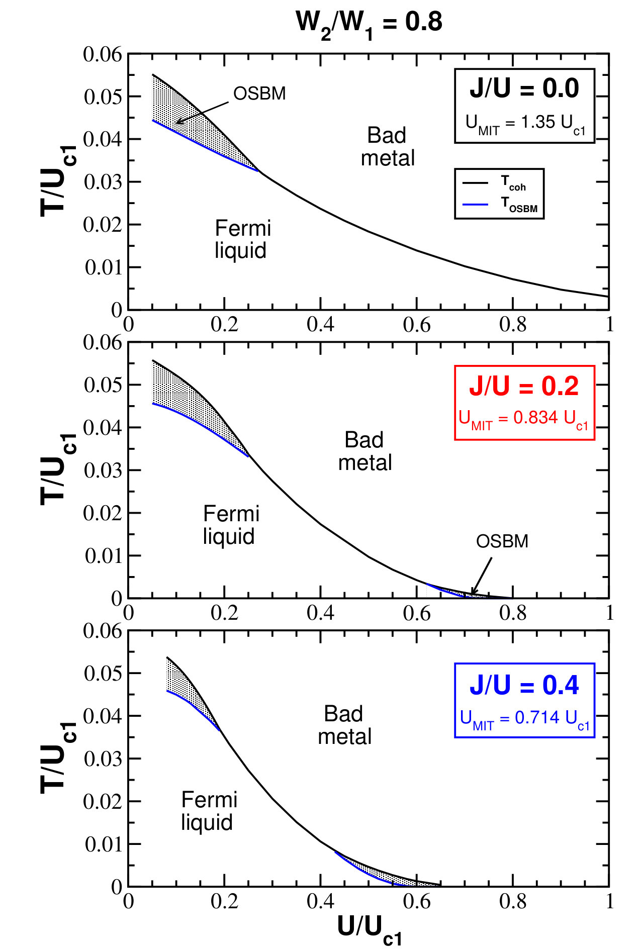 Figure 1
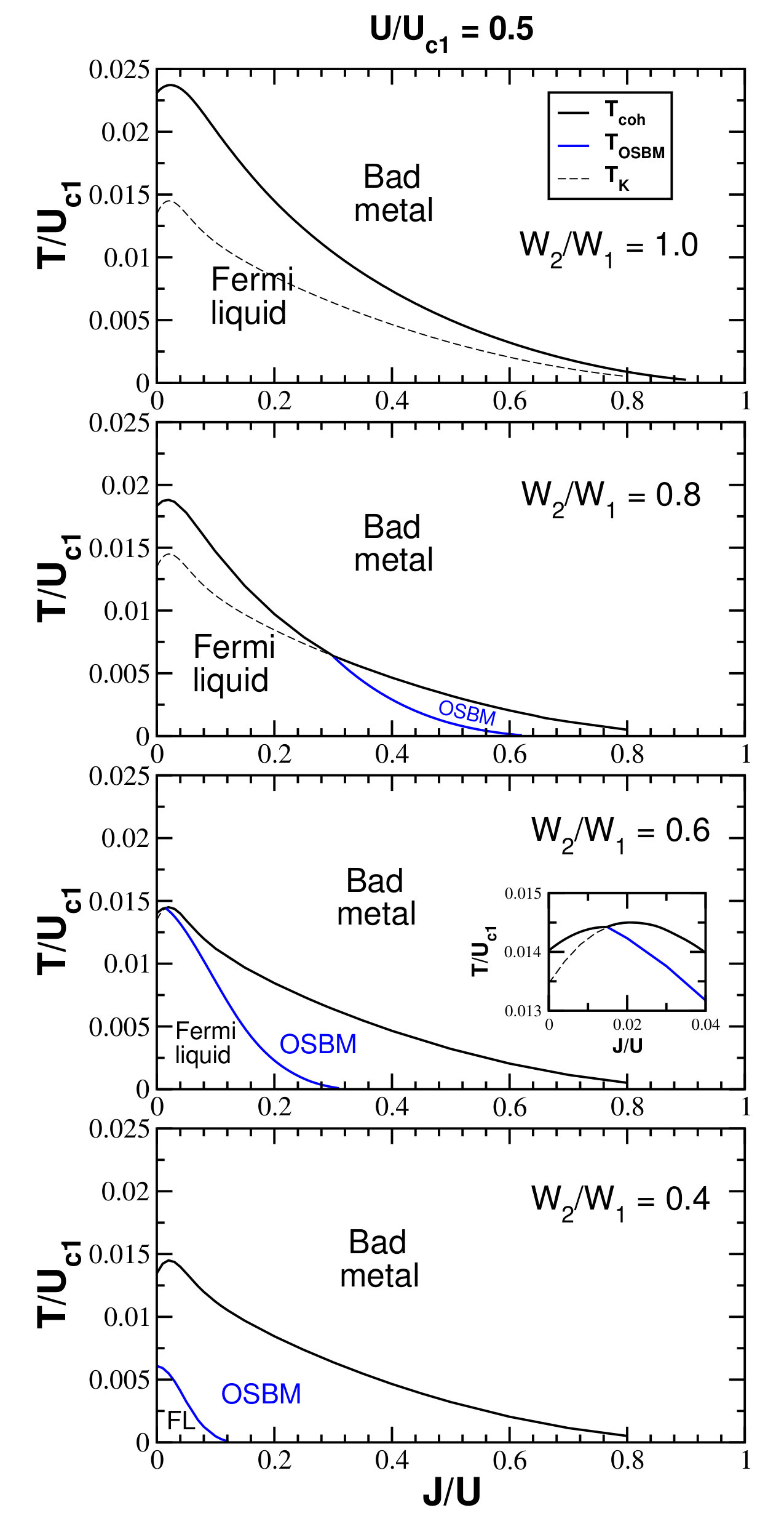 Figure 2
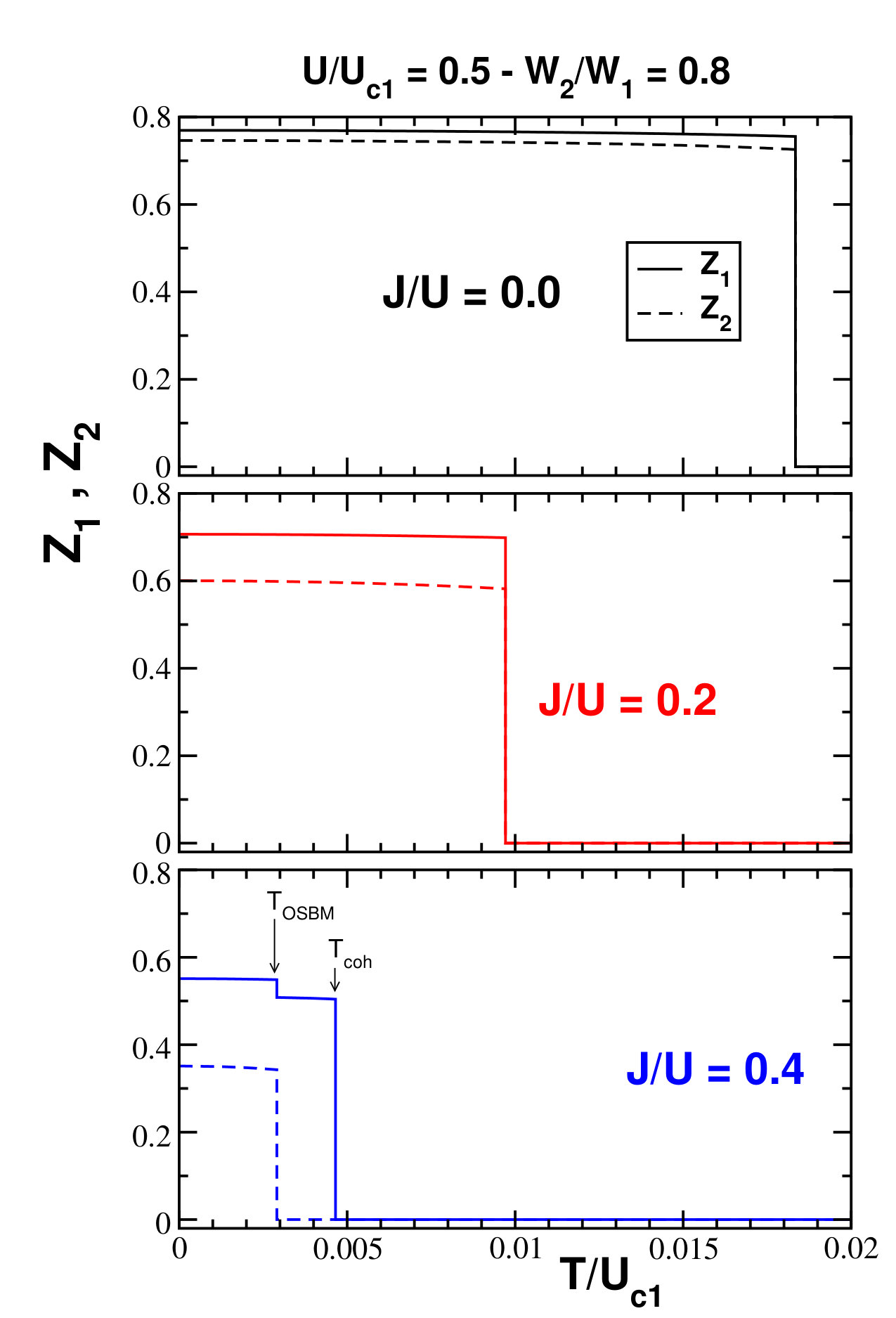 Figure 3
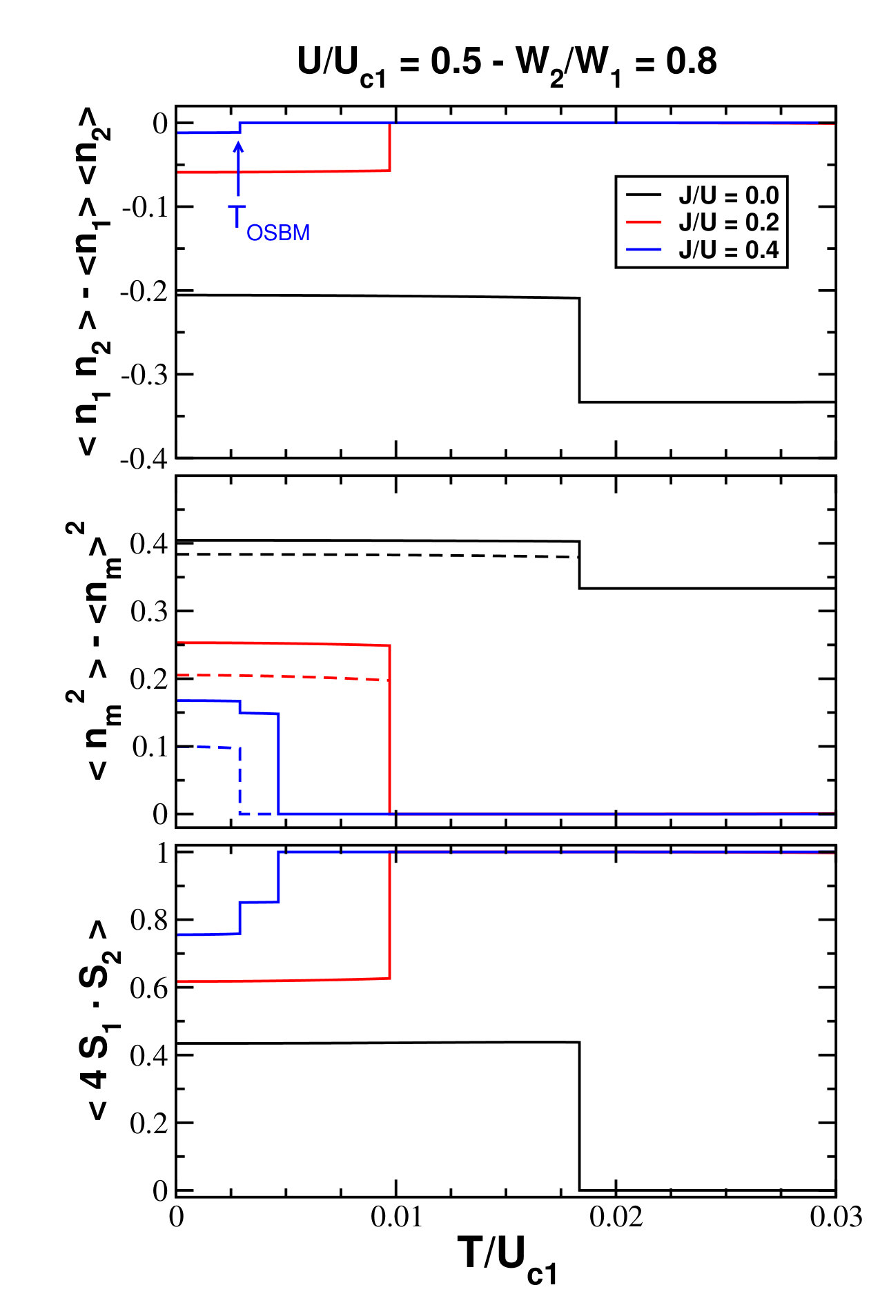 Figure 4
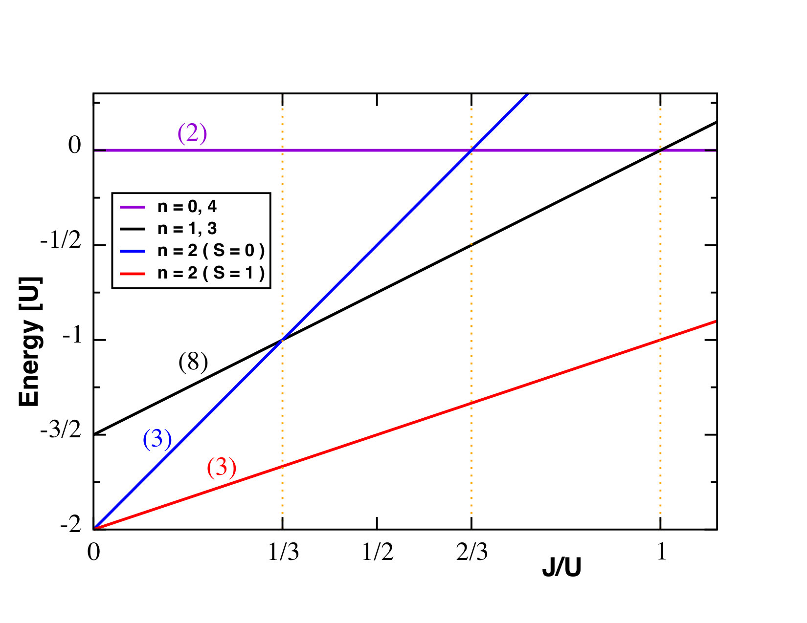 Figure 5
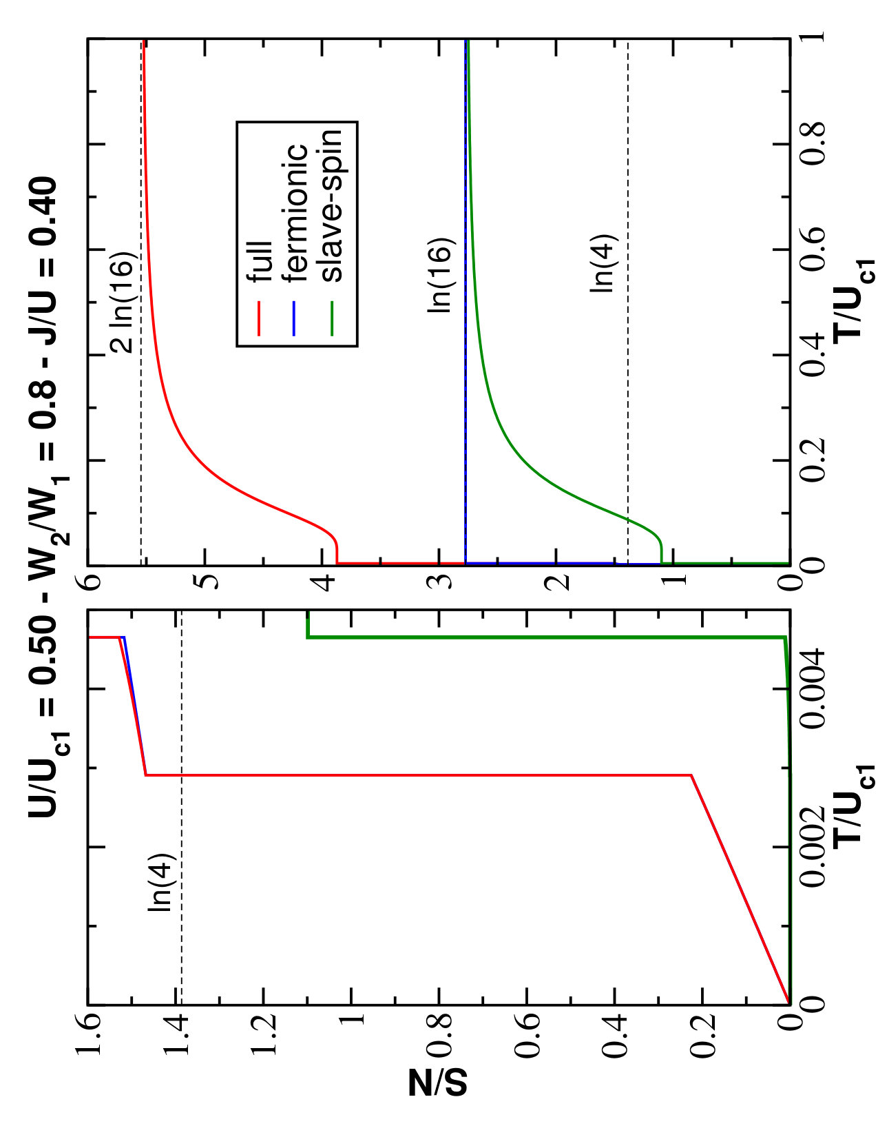 Figure 6
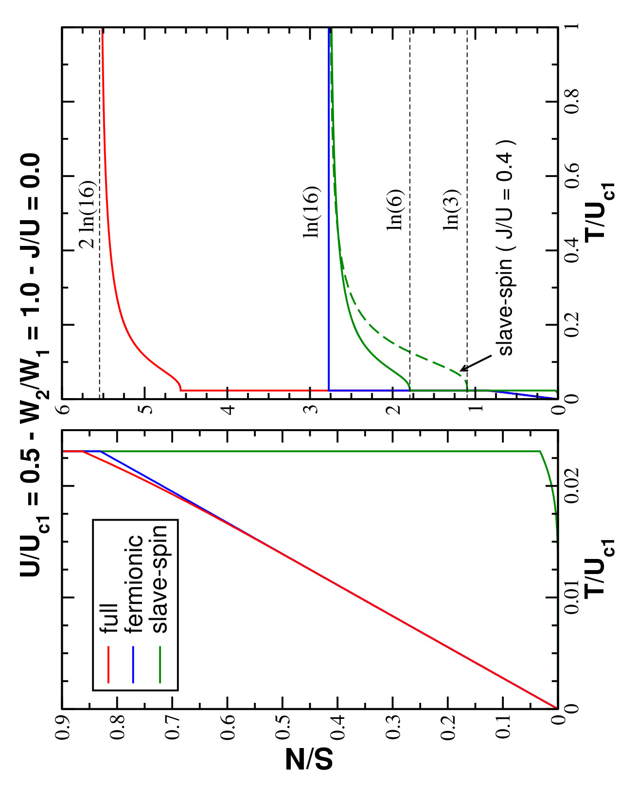 Figure 7
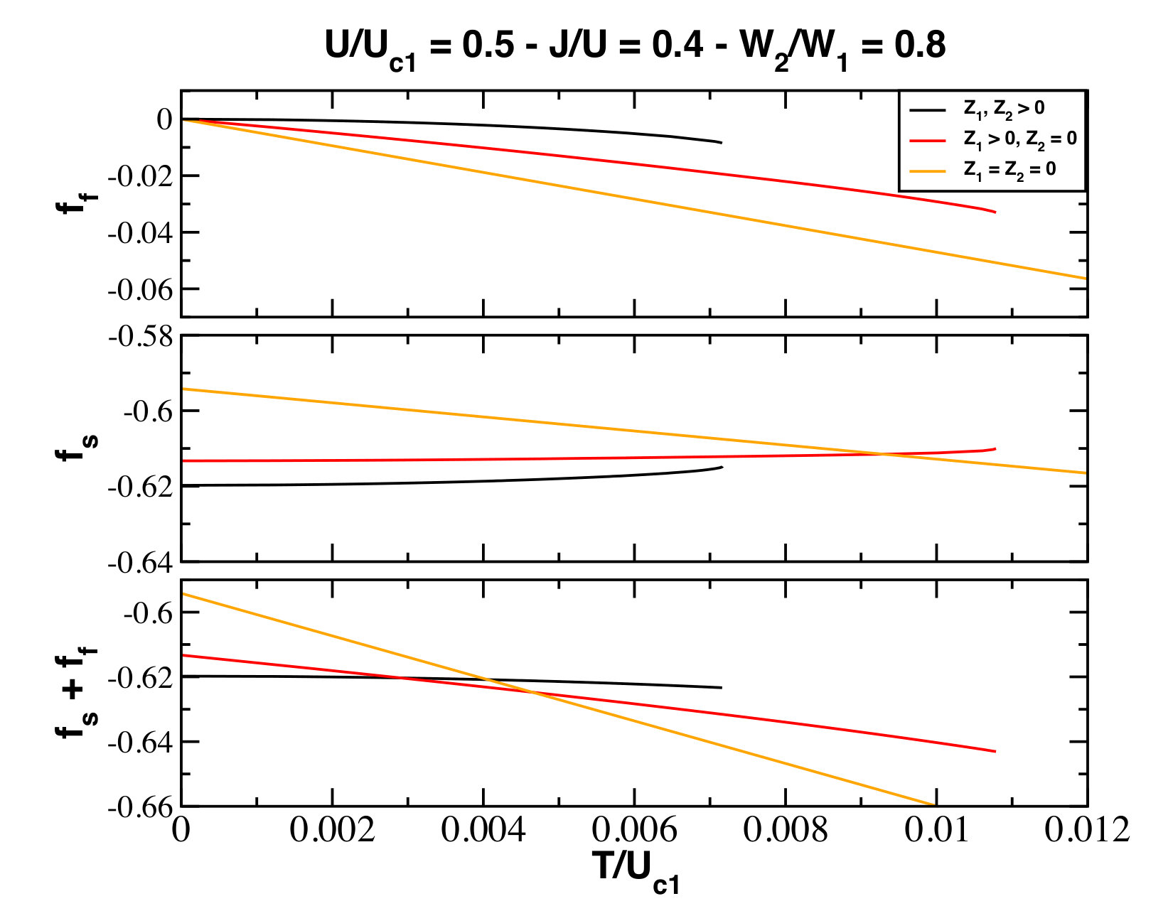 Figure 8
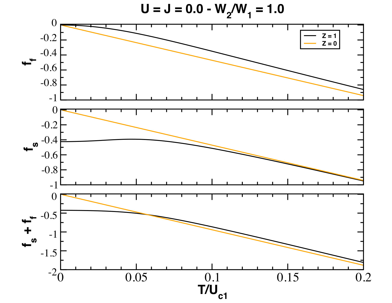 Figure 9
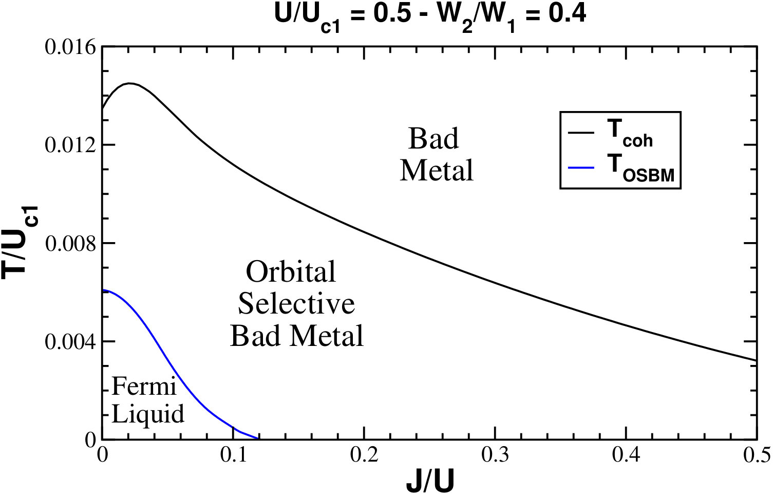 Figure 10
 Figure 11
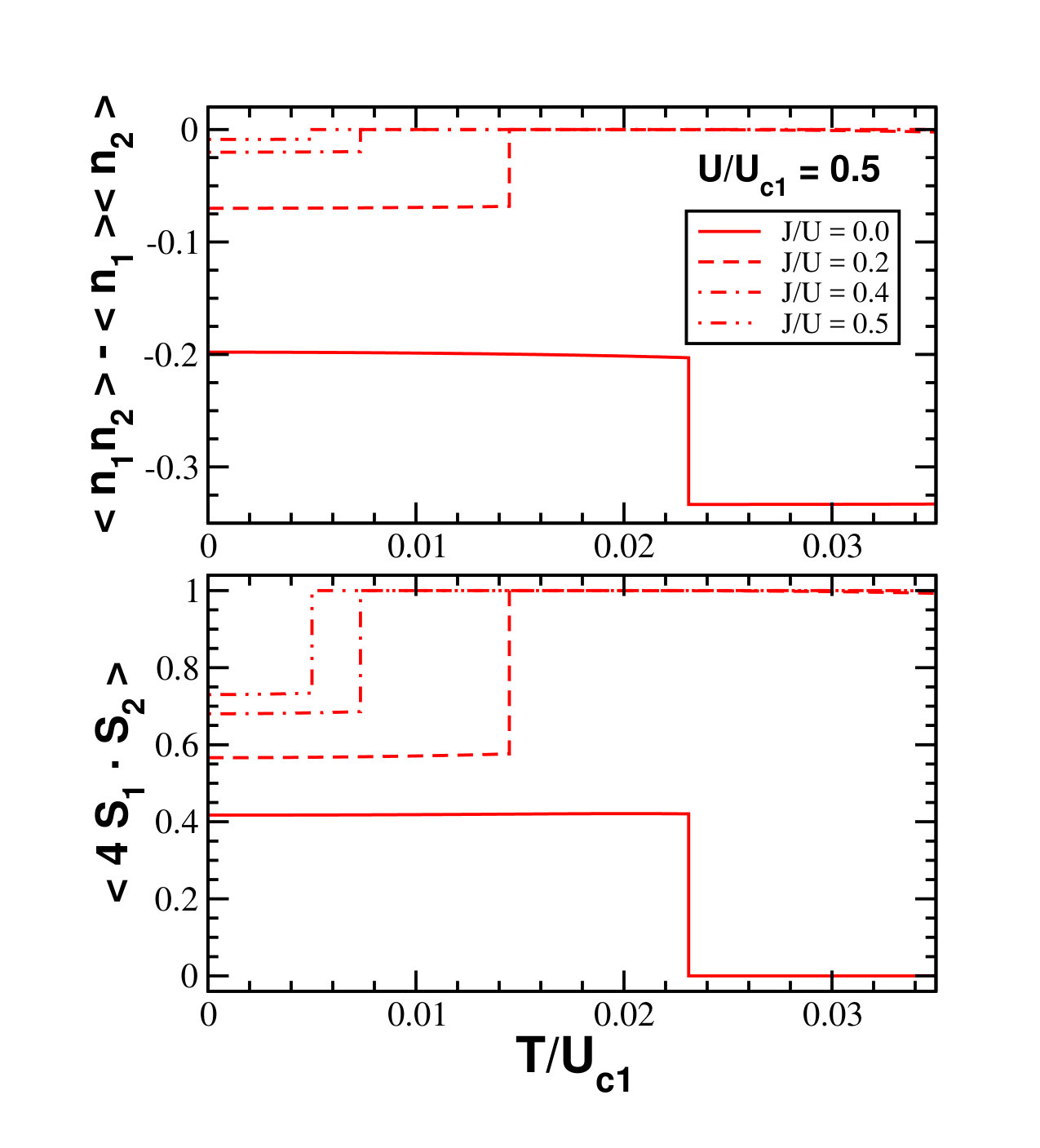 Figure 12
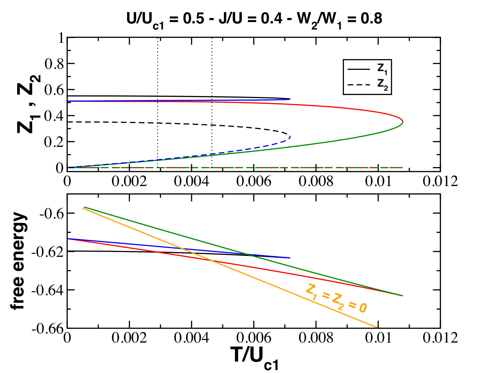 Figure 13
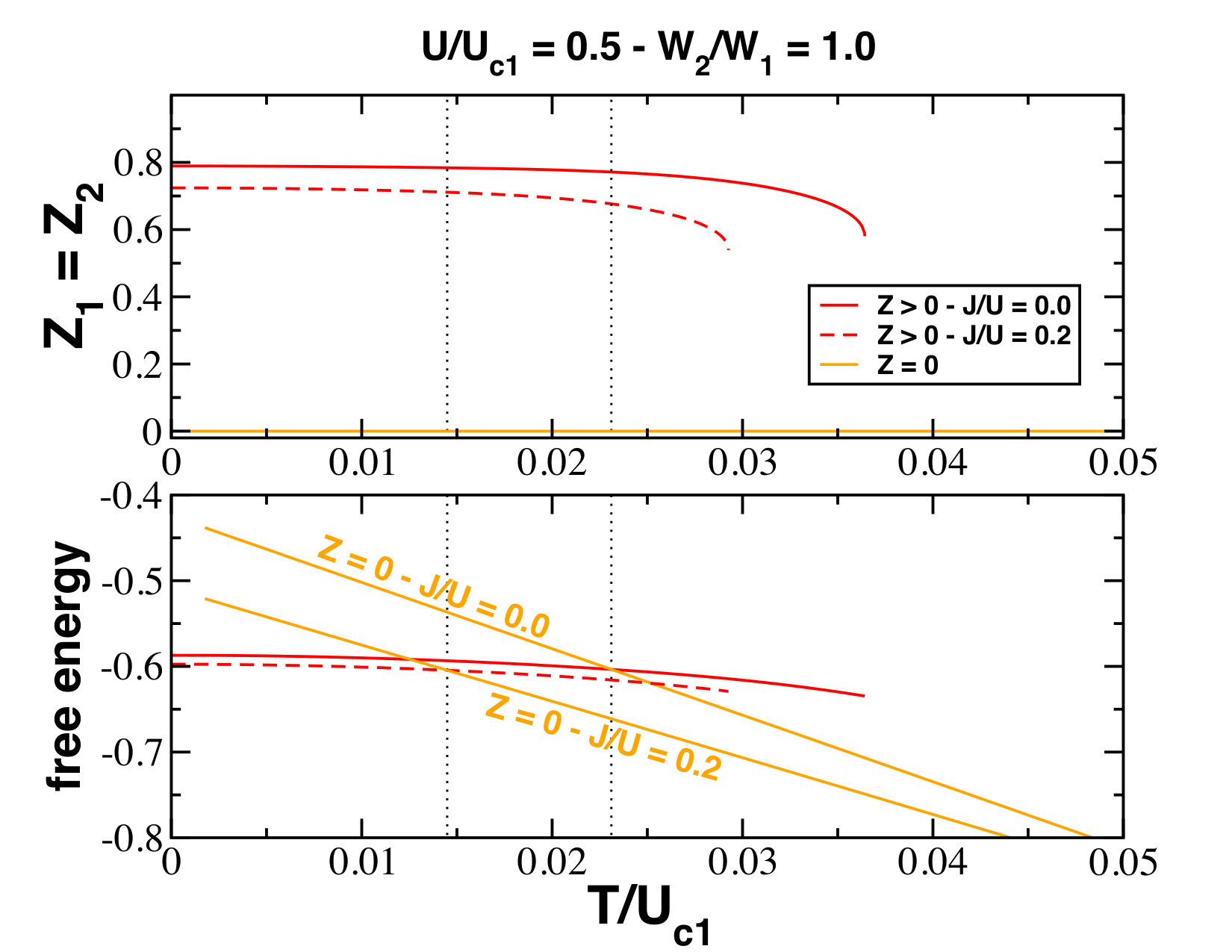 Figure 14
| State | Total spin | Energy | Energy (h-f) | |
|---|---|---|---|---|
Peer Reviews
No public reviews on file for this paper yet. If you reviewed it on a platform where reviews are public (OpenReview, ICLR, NeurIPS, ICML), you can paste yours below so the community can read it here.
Videos
No videos yet. Explain this paper in a talk, walkthrough, or lecture? Add one.
Orbital-selective bad metals due to Hund’s rule and orbital anisotropy: a finite-temperature slave-spin treatment of the two-band Hubbard model
Alejandro Mezio
School of Mathematics and Physics, University of Queensland, Brisbane QLD 4072, Australia
Ross H. McKenzie
School of Mathematics and Physics, University of Queensland, Brisbane QLD 4072, Australia
Abstract
We study the finite-temperature properties of the half-filled two-band Hubbard model in the presence of Hund’s rule coupling and orbital anisotropy. We use the mean-field treatment of the slave-spin theory with a finite-temperature extension of the zero-temperature gauge variable previously developed by Hassan and de’ Medici [Phys. Rev. B 81, 035106 (2010)]. We consider the instability of the Fermi liquid phases and how it is enhanced by the Hund’s rule. We identify paramagnetic solutions that have zero quasi-particle weight with bad metallic phases, and the first-order transition temperature between it and the Fermi liquid phase as a coherence temperature that signals the crossover to the bad metallic state. When orbital anisotropy is present, we found an intermediate transition to an orbital-selective bad metal (OSBM), where the narrow band becomes a bad metal while the wide band remains a renormalised Fermi liquid. The temperatures and at which the system transitions to the bad metal phases can be orders of magnitude less than the Fermi temperature associated with the non-interacting band. The parameter dependence of the temperature at which the OSBM is destroyed can be understood in terms of a ferromagnetic Kondo-Hubbard lattice model. In general, Hund’s rule coupling enhances the bad metallic phases, reduce interorbital charge fluctuations and increase spin fluctuations. The qualitative difference found in the ground state whether the Hund’s rule is present or not, related to the degeneracy of the low energy manifold, is also maintained for finite temperatures.
I Introduction
One of the most interesting new ideas about quantum matter from the last decade is that of a Hund’s metal.Yin2011; Haule2009a; Georges2013a; DeMedici2017b This is a strongly correlated metal that can occur in a multi-orbital material as a result of the Hund’s rule interaction , that favours parallel spins in different orbitals. While strong correlation effects are often associated with the proximity to a Mott insulating state, it has become clear in recent years that the Hund’s rule coupling (rather than the Hubbard ) is responsible for strong correlations in multiorbital metallic materials that are not close to a Mott insulator, such as the iron-based superconductors,Haule2009a; Yin2011 and ruthenates.Werner2008; Mravlje2011 Besides the enhanced electron correlation, this new type of strongly correlated system is characterised by local high spin configurations with slow dynamics and selectivity of the electron correlations depending on the orbital character.Werner2008; Haule2009a; DeMedici2017b Hund’s coupling considerably reduces the low-energy quasiparticle coherence scale, that results in an incoherent metallic state with frozen local moments in an extended temperature range above it, i.e., a bad metal.
It has been shown that Hund’s rule has a conflicting effect on the correlations of multiorbital systems. At integer fillings, its modifies the critical interaction where the metal-insulator transition (MIT) occurs, , depending on the number of electrons per site,DeMedici2011a; Georges2013a and reduces the temperature scale above which a bad metal is formed.Haule2009a; Ong2012 In the one band Hubbard model, this coherence temperature is orders of magnitude smaller than the bare energy scales of the system ( and bandwidth ) and signals the breakdown of the low-temperature Fermi liquid (FL) picture and the crossover to a bad metal state. Several other signatures of this FL to bad metal crossover at exist: the resistivity becomes of order of the Mott-Ioffe-Regel limit (), an incoherent electron spectral function, a collapse of the Drude peak in the optical conductivity and a shift of the associated spectral weight to higher energies, the entropy and specific heat become of order per particle, the NMR Knight shift dependence with the temperature becomes consistent with a local-moments dominated behaviour (Curie-Weiss), and sometimes there is a nonmonotonic temperature dependence of the Hall coefficient and thermoelectric power.Rozenberg1995; Merino2000; Gunnarsson2003; Hussey2004a; Merino2008; Deng2013a; Xu2013; Vucicevic2013; Vucicevic2015; Dasari2016b Usually associated with the proximity to a Mott MIT, it is interesting to ask how and why the Hund’s rule interaction and orbital degeneracy and character change this low-temperature crossover and enhance the formation of bad metals.
When orbitals have different bandwidths or their degeneracy is lifted by a crystal field, correlations can affect each band differently. Some orbital-dependent correlations have been investigated in theoretical calculations for iron-based superconductorsDeMedici2009; Ishida2010; Yu2011; Bascones2012; Yu2012; Georges2013a; Yi2013; Yu2013; Terashima2013; DeMedici2014; Liu2015; Yi2015 and ruthenates.Anisimov2002; Koga2004; DeMedici2005; Mravlje2011; Georges2013a Hund’s rule decouples the orbitals, enhancing such orbital differentiation,DeMedici2005; DeMedici2009; DeMedici2011; Yu2013 and an extreme case occurs at when some orbitals transition to a Mott phase while others remain metallic, leading to an orbital-selective Mott phase (OSMP).Anisimov2002; Liebsch2004; Koga2004; DeMedici2005; Ferrero2005; Inaba2007a The two-band Hubbard-Kanamori model with unequal bandwidths is the simplest model where a transition to an OSMP occurs,Anisimov2002; Koga2004; DeMedici2005; Ferrero2005; Liebsch2005; Biermann2005; Werner2007a; Vojta2010 and some earlier numerical works using dynamical mean-field theory (DMFT) explore its effects at finite temperature.Liebsch2004; Biermann2005; Knecht2005; Liebsch2005; Inaba2005; Liebsch2006; Inaba2007
Based on scanning tunnelling microscope (STM), recent quasi-particle interference measurements of the normal state Fermi surface and superconducting energy gaps on FeSe, give support to the idea that orbital-selective strong correlations dominate the parent state of iron-based superconductors.Sprau2017a; Kostin2018 Including these values of orbital-selective quasiparticle weights into a spin-fluctuation pairing theory in a random-phase approximation (RPA) study, some of the authors of the previous papers obtain an accurate description for the superconducting gap, indicating the key role of orbital-selective Cooper pairing.Sprau2017a; Kreisel2017 And more recently a good agreement in the calculated magnetic excitation spectrum with inelastic neutron scattering experiments in FeSe.Kreisel2018
Angle-resolved photoemission spectroscopy studies on several iron-based superconductors show a temperature-induced crossover from a metallic FL state at low temperature with well-defined Fermi surfaces for all the bands, to a phase where the orbital loses spectral weight with increasing temperature and the associated Fermi surface dissapears. See Ref. Yi2013 for results in Fe2-ySe2 ( = K, Rb); Ref. Yi2015 for FeTe0.56Se0.44, K0.76Fe1.72Se2 and FeSe grown on SrTiO3; Ref. Liu2015 for Fe1+ySexTe1-x (); Ref. Pu2016 for single layer FeSe/Nb:BaTiO3/KTaO3; and Ref. Miao2016a for LiFeAs. These results indicate an orbital-differentiated coherent-incoherent crossover, and are consistent with a scenario of a Kondo-type screening determined by the strength of the Hund’s rule coupling. Other experimental probes also find a coherent-incoherent crossover, with signatures of a bad metal behaviour: temperature dependence of the Knight shift consistent with a Curie-Weiss behaviourWu2016 and strong temperature dependence of the Hall coefficientXiang2016a in Fe2Se2 ( = K, Rb, Cs), and a collapse of the Drude peak in the optical conductivity of KFe2Se2, where spectral weight is transferred from low to high energy.Yang2017a
An important question concerns the extent to which slave-particle mean-field theories can capture the stability of the Hund’s metal and its properties, including the emergence of a bad metal above some coherence temperature, . In the single-band Hubbard model, the strongly correlated metallic phase that occurs in proximity to a Mott MIT is associated with a small quasi-particle weight and suppression of double occupancy, reflecting suppressed charge fluctuations. This is captured by slave-boson mean-field theory, including the small coherence temperature.Dao2017; Mezio2017 In contrast, the strongly correlated Hund’s metal is associated with suppression of singlet spin fluctuations on different orbitals, without suppression of onsite charge fluctuations, and is seen with the slave-spin mean-field (SSMF) theory at zero temperature.Fanfarillo2015; DeMedici2017; DeMedici2017a To the best of our knowledge, there is no work studying an extension of this SSMF theory to finite temperatures, but only using other variants of the method.Yu2013d; Yi2013; Gao2014; Yi2015; Yang2018
In this paper, we propose a finite-temperature implementation of the SSMF theory that is a natural extension of the formulation,Hassan2010; DeMedici2017a and we apply it to the two-band Hubbard-Kanamori model at half-filling. We explore the effects of the Hund’s rule and orbital anisotropy in the coherence temperature , and the inter-orbital spin and charge fluctuations. We also investigate the appearance of an orbital-selective bad metal phase, where one band has incoherent quasiparticles, i.e., bad metal, while the other remains a FL. Fig. 1
shows the phase diagram for vs for the two-band Hubbard Kanamori model with different orbital bandwidths and at intermediate interaction , and summarises our main result. The Hund’s rule interaction enhances the stability of the orbital-selective bad metal phase, strongly reducing the (first) coherence temperature . It also increases correlations, reducing the (second) coherence temperature , where the remaining metallic band becomes a bad metal. At , a transition from the FL to an OSMP occurs at a critical value of the Hund’s coupling . In this way, even for low- the system is close to an orbital-selective Mott phase, and an increase in temperature favours the OSBM phase. This occurs even in the case of small anisotropy (see Fig. 7).
It is worth clarifying that previous SSMF studies at identify the slave-spin paramagnetic phase where the quasiparticle weight is with a Mott insulator phase, while it has been pointed out that beyond the single-site approximation this might be an orthogonal metal, a type of fractionalised non-Fermi liquid.Nandkishore2012 In our paper we use the single-site mean-field approximation (valid in the large dimension limit). Although our results in the slave-spin paramagnetic phase can suggest a complex behaviour (e.g., see Sec. III.3), the temperature dependence of this phase follows a simple thermal activation of the atomic slave-spin states.
The organization of the paper is as follows: In Sec. II, we describe the Hubbard-Kanamori model and SSMF method. Details on the finite- implementation are in Appendix A. In Sec. III, we present our results for the temperature dependence of the quasiparticle weight, coherence temperature, spin and charge fluctuations, phase diagrams and entropy contributions. We identify the first-order transition temperature where the quasiparticle weight vanishes to the coherence temperature associated with the crossover to a bad metal. The behaviour of is qualitatively different whether the Hund’s rule coupling is present or not, as it is found for the ground state and explained from the degeneracy of the low energy manifold.Koga2004; DeMedici2017a We found that the change of when moving occurs only through the modification of the zero- critical interaction where the MIT occurs, . When orbital anisotropy is present the width of the two bands are unequals (i.e. ), and we found that the Hund’s rule facilitates the first-order transition from the FL to a state where the narrow band quasiparticle weight vanishes. We identify this with a crossover to an orbital-selective bad metal state and this additional coherence temperature as . Details on the construction of the solutions and an analysis of the atomic states are in Appendices B and C, respectively.
II Model and Method
II.1 Model Hamiltonian
Our starting point is the general multi-band Hubbard-Kanamori HamiltonianGeorges2013a which describes interacting electrons in orbitals,
[TABLE]
where,
[TABLE]
is the non-interacting term, and the total number of electrons. As usual, creates an electron with spin at the site on the orbital , and is the occupation for the site . The hopping matrix element satisfies , has no inter-orbital hybridisation (), and we write out explicitly the orbital energies (). The interaction terms are,
[TABLE]
where we omit the site label . The density-density term involves the on-site Coulomb interaction between electrons in the same orbital with opposite spins , in different orbitals with opposite spins , and different orbitals with parallel spins ; while involves the spin-flip () and pair-hopping () interactions.
The model has rotational symmetry whether one chooses and , or sets , and . Although the former case refers to the physical Hamiltonian for states, the choice does not affect the results qualitatively and for simplicity we use the latter set of parameters.Georges2013a; Komijani2017 We restrict our results to the two band case () at half-filling (), each with orbital energy , bandwidth and a semicircular density of states,
[TABLE]
Several previous works studied the two-band model at zero temperature with the slave-spin method, calculating its different phases and its dependence with Hund’s coupling, orbital anisotropy, crystal field splitting, orbital hybridisation, and different fillings.DeMedici2005; Hassan2010; DeMedici2011; Komijani2017; DeMedici2017a We use those results as a guide to benchmark our results when , and focus on how , and the orbital anisotropy affects the system at finite temperature.
Throughout the paper we use the one-band critical interaction as the energy unit,
[TABLE]
which is the only relevant energy scale for the one band case at the mean field level.Mezio2017 It depends only on the zero- uncorrelated kinetic energy , that we define later on Eq. (15). An extension of this energy scale for generic filling is .Mezio2017
II.2 Slave-spin mapping
We use the slave-spin mean-field (SSMF) method DeMedici2005; Hassan2010; Georgescu2015; DeMedici2017a to study the finite temperature behaviour of the Hubbard-Kanamori Hamiltonian (1). This method involves a slave-particle representation where we express the physical electron as a product of a fermion and slave spin- operator, allowing a rewriting of the Hamiltonian more suitable for further mean-field approximations. Here the slave-spin states “up” or “down” labels occupied or unoccupied electronic states, respectively. Within this mapping, the operators in the non-diagonal part of are replaced by,
[TABLE]
where is an auxiliary fermion operator, and is a generic slave-spin operator. Its general form is,
[TABLE]
with an arbitrary complex number that we can tune after an approximation scheme to reproduce solvable limits of the problem. At and single-site mean-field level, a set of choices for this parameter that recover the physical solution in the uncorrelated limit and work for generic filling,Hassan2010; DeMedici2017a give interesting results and have been thoroughly tested against DMFT, slave-boson and Gutzwiller approximations.DeMedici2005; DeMedici2009; Hassan2010; DeMedici2011; DeMedici2014; Fanfarillo2015; DeMedici2017a However, it fails to satisfy the non-interacting limit when used at finite temperature. In this paper, we develop an extension of this choice of (real) -parameter suitable for finite temperatures. Details of the calculation are in Appendix A.
For the application of the slave-spin mapping on the other terms of the Hamiltonian (1), it is convenient to rewrite the density-density Hamiltonian in a particle-hole symmetric form. For this, we shift all the number operators in by , . By doing this, we only add a one-body term that shifts the chemical potential, , and a constant total energy shift, , where,
[TABLE]
for two bands and our choice of parameters. These displaced number operators in have the same quantum numbers and are mapped to the -component slave-spins operators, . The electron number operators that are not shifted by , i.e., those accompanying and , are represented by the auxiliary fermion occupation operator, . Finally, in Eq. (4) mixes the Hilbert spaces of the fermions and slave-spins, and we use here the approximate mapping and , which has the correct slave-spin quantum numbers and captures the spin-flip and pair-hopping physics in that Hilbert space.DeMedici2005; DeMedici2017a
Due to the increase in the size of the Hilbert space by slave-particle methods, constraints must be introduced to reproduce the physical states by the auxiliary ones. In the slave-spin formulation we only need one constraint equation per introduced slave-spin degree of freedom, namely
[TABLE]
II.3 Mean-field approximation
Following Reference [DeMedici2017a], we perform a mean-field decoupling for each site between the fermionic and slave-spin degrees of freedom, , followed by a single-site mean-field in the slave-spin operators, . The constraints in Eqs. (10) are included through a Lagrange multiplier by adding the term to the Hamiltonian (1) . Finally, we assume translational invariance (, and ) and paramagnetic solutions (, and ).
After the mean-field approximations and assumptions, the Hamiltonian separate into a Hamiltonian on non-interacting fermions,
[TABLE]
and a purely slave-spin single-site Hamiltonian , with
[TABLE]
where is the hopping renormalisation factor and the quasiparticle weight for the orbital , and , with
[TABLE]
the average electronic kinetic energy of the band . Here is the dispersion relation of the uncorrelated -orbital, its bare density of states, is the Fermi function for the orbital occupation per spin, and is the Fourier transform to the reciprocal space for the fermionic operators. For convenience, we take the parameter in to be real, hence is real too, and .Hassan2010; DeMedici2017a
The total Hamiltonian, without taking into account the and energy shifts, is , where
[TABLE]
is the energy per site of the hopping Hamiltonian at the mean-field level. The free energy density is , with the partition function for one site,
[TABLE]
The first line of Eq. (17) is due to the fermionic degrees of freedom, the middle one is the slave-spin part with its one-site partition function, and the bottom term is the mean-field energy of the hopping term. By minimising against the mean-field parameters and , we obtain the self-consistent equations,
[TABLE]
where is the expectation value calculated on the slave-spin Hilbert space, and is solved by diagonalising the matrix for the single-site Hamiltonian .
In the Appendix A we calculate the finite temperature extension of the real choice of the -parameter for one band. We obtain a self-consistent equation that depends on the -parameter, the temperature , the uncorrelated kinetic energy for one band, i.e., , and the occupation number of the band in the non-interacting limit . The SSMF yields a non-zero Lagrange multiplier in the uncorrelated limit, ,DeMedici2014; DeMedici2017; DeMedici2017a an unwanted behaviour that is solved by shifting to satisfy the physical non-interacting limit . Previous works use a numerical calculation of to perform this shift. In our case, we obtain in Eq. (25) an analytic expression for that depends on , and , and use it throughout our calculations.
In the multiorbital case, the non-interacting limit is just a set of uncoupled one-band systems, and each orbital has its and determined by , , and its non-interacting occupation number . For a fixed temperature and total occupation of the site , the iteration scheme used is: (i) calculate the non-interacting chemical potential through , and consequently each orbital occupation and kinetic energy (ii) set the value of using the self-consistent equation, and consequently the value of , and (iii) solve the self-consistent Eqs. (18) and (19) for and .
III Results
III.1 Isotropic case ()
III.1.1 Quasiparticle weight and coherence temperature
For fixed , we show how increasing drives the metal close to the Mott insulating phase and reduces the coherence temperature. In the top of Fig. 2
we plot in red the quasiparticle weight for half-filling, and vary . In thin dotted lines we plot the solutions with finite in the whole range of temperature where they are found to exist. These solutions are the ones that evolve continually from the zero- results. For each case, at the free energy of this finite- solution crosses with the one corresponding to the “trivial” solution with , and the later becomes the stable phase for . For a description of the construction of the physical solution refer to Appendix B. For the quasiparticle weight is almost constant, slightly decreasing with increasing , and jumping to zero at . We identify this temperature with the coherence temperature of the fermionic quasiparticles, associated with the crossover to a bad metallic state.
It is known that the effect of the Hund’s coupling in multiorbital systems at half-filling is to increase correlations, and increasing and/or reduce the values of and ,DeMedici2011a; Georges2013a enhancing the stability of the bad metal. But the reduction in the coherence temperature is more pronounced than the reduction in the quasiparticle weight, showing that the reduction of is not just due to band renormalisation.Mezio2017 We also add in blue the solution for and , that has the same quasiparticle weight at zero- as the and case. A similar increase in correlations at , due to or , gives a slightly different reduction of . This difference decreases when correlations are stronger (bigger and/or ) and the system gets closer to a MIT, and we can conclude that regarding there is no big difference here between the increase of correlations through or . Although, there is a qualitative difference between the and case, that we discuss below.
In the bottom of Fig. 2 we plot the phase diagram for temperature vs interaction and how it changes with increasing . The solid lines are the coherence temperature associated with the crossover to a bad metal regime. We can see that the SSMF method obtains a very low coherence temperature close to the Mott MIT, as expected for strongly correlated materials. The inset of Fig. 2 shows the same plot, but with normalised to its value at the metal insulator transition, . We can see that the case is qualitatively different from those with finite , whereas for the latter becomes independent of the particular value of , and only depends on the relative position of to its zero- metal insulator transition value. In other words, for two equal bands only depends on through its effect on the zero temperature critical interaction .
It is useful to focus on the atomic configurations to understand the difference between zero- and finite-. A detailed list of the atomic states and its energies is in Appendix C. At half-filling, it is easy to check from Eqs. (3) and (4) that the states with two electrons onsite have the lowest atomic energy.Koga2004; DeMedici2011; Komijani2017 For , this low atomic energy sector is six-fold degenerate with energy , and has states with total spin per site and . While for , this degeneracy is lifted into the two different spin sectors, each of them now three-fold degenerate. Here, the triplet sector has the lowest atomic energy, . This change in the degeneracy and total spin of the lowest energy manifold is the causes of the different behaviour of the ground state for and ,Koga2004; DeMedici2017a and consequently, cause the different behaviour observed in this work at low temperature.
The sector next in energy is , which have one/three electrons per site and is eight-fold degenerate. For we have that , but this inequality is reversed when (see Fig. 14) and we can expect a change in the finite temperature behaviour. We find no qualitative change when crosses this value and, as discussed before, the quasiparticle weight has an almost constant value for . This tells us that the effective temperature is much lower than any energy scale of the system and, within this range of temperatures the system lives mostly in the low energy manifold.
III.1.2 Charge and spin fluctuations
The calculation of spin and charge fluctuations is helpful to clarify the different nature of the correlations, either due to an increase of or .Fanfarillo2015 We remember here that the occupation operator of the orbital is and the -component of its physical spin is , and we use the constraint Eq. (10) to write them in the slave-spin Hilbert space. The transversal components of the physical spin are also easy to express in the local slave-spin basis. In this way, in Fig. 3
we plot the on-site inter-orbital charge (top) and spin (bottom) fluctuations, and , respectively. Here stands for the spin operator of the orbital on the site, .
Regarding the inter-orbital charge fluctuations (top of Fig. 3), they are negative for , as expected for repulsive interactions in a FL. As it is known from Mott physics, an increase of correlations localise electrons on sites and suppresses charge fluctuations. But again, the effects are different whether we increase correlations through or .Fanfarillo2015 The increase of the Hund’s coupling polarizes the spin on the site and increase the energy gap between and , restricting the system to the triplet configurations, and making the inter-orbital charge fluctuations approach to zero. At the transition a jump to zero (for ) at the trivial solution occurs, where this state can be understood within the method as two flat bands interacting each other through an effective ferromagnetic interaction. On the other side, for , increasing correlations via the Coulomb interaction makes the inter-orbital charge fluctuations of the FL phase approach to the value (not shown in plot). We can understand this by noting that, if we restrict ourselves to the six-fold degenerate manifold, two states have and the other four , obtaining a total that account for the value in the charge fluctuation quantity (see Appendix C). The next available states are at an energy gap of , and are accessible to the system through the hopping Hamiltonian. Finally, increasing towards the MIT makes this gap bigger and the system more restricted to the lowest energy manifold, where we shown that . We can interpret the jump to in the line in a similar way: the transition at to the trivial phase with cancels the effect of the hopping Hamiltonian, restricting the system to the lowest manifold and obtaining the value at low temperatures. When increased further the temperature, at around thermal transitions to other available states occur, making the inter-orbital charge fluctuation to approach slowly to zero (not shown in plot).
The spin fluctuations (bottom of Fig. 3) grow with increasing , as expected for the spin polarisation due to Hund’s coupling. The value is the correct limit for the picture of a ground state lying in the manifold. Similar arguments as before apply for the transition to the trivial state for , where two flat bands are coupled with and have a low temperature value . For in the trivial state there are no interactions between the spins and . We can say that for there is a qualitative difference in spin-triplet correlation between and . Finally, further increase in the temperature washes out the effect of on the trivial states, and at high temperatures we approach the limit (not shown in plot).
III.2 Anisotropic orbitals
We explore now the effect of the Hund’s coupling at finite temperature when we have an orbital anisotropy, , i.e., the two bands have different widths. We will see how an orbital-selective bad metal becomes possible.
III.2.1 Quasiparticle weights, coherence temperatures and fluctuations
In Figure 4
we show the quasiparticle weight for orbital (solid lines) and (dashed lines), where the bandwidth anisotropy is and , for three values of Hund’s coupling, , and . Same as before, the dotted lines show the different solutions in the whole temperature range they are found, and we set the different first-order transitions where the different free energies crosses each other (see Appendix B). The increase of correlations affects more to the narrow orbital, as we can see from the stronger renormalisation of when increases. Although the orbital anisotropy is mild, with we find an intermediate transition to a solution with and . Following our previous interpretation, here the narrow orbital transitions to a bad metal state while the wide orbital remains FL, although it suffers a renormalisation in the quasiparticle weight . We call this phase an orbital-selective bad metal (OSBM), and the transition temperature . Further increasing temperature, another first-order transition occurs at , where the wide orbital also collapse and both bands are in a bad metal state. For this value of the correlation , an increase of stabilizes the OSBM phase.
The physics of this new phase is better understood from the charge and spin fluctuations, which we show in Figure 5.
From top to bottom we have inter-orbital charge, intra-orbital charge, and inter-orbital spin fluctuations. In black, red and blue we show result for , and , respectively. Solid and dashed lines in the middle plot refers to wide and narrow orbitals, respectively. For the inter-orbital charge fluctuations (top) we have the same general behaviour as in the isotropic case of the previous section. The new aspect is that for the jump to zero occurs at the transition to the OSBM phase, at . This means that charge movement between orbitals cancels when the narrow orbital collapses. The narrow orbital is completely localised in this phase, and interaction with the FL of the wide orbital is only through the spins and the Hund’s rule coupling. The intra-orbital charge fluctuations (middle) shows clearly that when the wide band is still metallic (solid blue line) while the narrow band has . When the transition to the OSBM phase occurs, and the system is more restricted to the triplet configuration, which explains the rise on the spin fluctuations (bottom). The non-interacting limit () for these qunatities are: [math] for the inter-orbital, for the intra-orbital, and for the inter-orbital spin fluctuations.
III.2.2 Phase diagrams
We now consider how the transition temperatures to the bad metal () and the orbital-selective bad metal () vary as a function of the interaction strenghts and . In Figure 6
we plot for and different values of , the phase diagram for temperature vs interaction . The transition temperatures and are in blue and black, respectively, and the OSBM regions are shaded in grey. The first thing to notice is the appearance of an OSBM region at weak , which can be related to a weak inter-band coupling. The increase of reduces even further the inter-band coupling ( and ), and the low- OSBM region shrinks. Also, a high- OSBM region appears for finite-, which is the OSBM phase seen in Figs. 4 and 5 when . This region does not exist when and gets enhanced with increasing Hund’s rule coupling. We have now a more complete picture of how the Hund’s rule coupling enhances the OSBM phase, as discussed in the previous section, seen from two main effects: (i) the growth of the high- OSBM region with increasing , and (ii) the increase of correlations due to that strongly reduce and shift the OSBM region over the point. Similar to the inset in Figure 2 there is a qualitative difference between and when is normalised with (not shown in the plot), i.e., the vs lines for superpose each other and are different than the case.
In Figure 7
we plot for and different values of , the phase diagram for temperature vs Hund’s coupling . The transition temperatures and are in blue and black, respectively. The inset in is an enlargement of the low part. An increase in anisotropy enhance the region where an OSBM phase exist, and an increase in favours this phase when anisotropy is present. The vs line when an OSBM phase is present at lower temperatures is always the same, disregarding the value of . When entering the OSBM region, the narrow orbital becomes flat () and electron localise, while the wider orbital remains itinerant and interact with the full electron spin of the former through the Hund’s coupling. Considering the low energy physics of this phase the interaction cancels, and the effective Hamiltonian for the system is a ferromagnetic Kondo lattice with an additional Hubbard interaction () in the wide band.Biermann2005 In this sense, the coherence temperature is a Kondo temperature which does not depend on (dashed line in Fig. 7).
III.3 Entropy analysis
An interesting question is about how much of the temperature dependence of the entropy of the system can be captured by the SSMF method. The slave-spin mapping (7) increases the Hilbert space by the incorporation of a spin- degrees of freedom for every fermionic one, expanding it from a -dimensional to a -dimensional one. The constraint (10) removes any possible unphysical states, making the mapping exact. But at the mean-field level, we impose the constraint only on average, allowing the participation of unphysical states and more specifically their contribution to the entropy.
This is seen easily in the high temperature behaviour of the solid red lines in Figs. 8 and 9, where we plot the total entropy, incorporating all the degrees of freedom of the method. The entropy (per site) is calculated using the thermodynamic relation
[TABLE]
where is the free energy calculated in Eq. (17), and is the internal energy. The decoupling of the fermionic degrees of freedom from the slave-spin ones at the mean-field level allows us to separate their contribution explicitly. In the free energy, the first, second and third lines of Eq. (17) are due to the fermions, the slave-spins and the hopping mean-field energy (), respectively. The same occurs for , and we can separate the entropy in the fermionic and slave-spin contributions, , which are the blue and green lines, respectively, in Figs. 8 and 9.
Solid lines in Fig. 8 shows the isotropic case with and no Hund’s coupling. In the FL phase (left), for , we can see that the slave-spin contribution (green) is very small, which supports the atomic picture that the energy gap between the ground state and the low energy excitations is larger than the temperature scale in this range. The linear behaviour of the total entropy (red) in the FL phase is all due to the fermionic contribution (blue), whose physics is that of the free electrons in a renormalised band. For we are in the trivial phase with . Looking at the fermionic part of the free energy, we can think of as a renormalisation factor for the inverse temperature , and the trivial phase as the free fermion gas being in the infinite temperature limit with an entropy of . For the slave-spin contribution, the transition to the trivial state makes the entropy jump to , for (solid green), and to , for finite (dashed green). Here, the transition to vanishes the hopping terms between atomic states, and the system is restricted to the manifold where the ground state lives, which is six-fold and three-fold degenerate for and , respectively (see Appendix C). As expected, at other atomic states start to be accessed by thermal fluctuations and the slave-spin entropy approaches as is increased further.
In Fig. 9 we plot the same quantities for the case when an OSBM occurs. We have the same behaviour as for Fig. 8 respecting the FL phase () and the trivial phase (). For the intermediate OSBM phase, the narrow orbital collapse, , while the wide one remains metallic. This explains the jump in the fermionic entropy (blue), where the narrow orbital behaves as a free fermion gas ( implies infinite-temperature behaviour in orbital ). The slave-spin contribution starts to grow in the OSBM phase, but it remains very small.
IV Concluding remarks
In conclusion, we have used the slave-spin mean-field method to study the two-band Hubbard system at finite-temperature in the presence of Hund’s rule coupling and band anisotropy. We have developed a finite- extension of the single-site approximation of the zero- formulation, that reproduces the physical limit for the uncorrelated case. We have identified the temperature where the first-order transition between finite- to solutions occurs with the coherence temperature that signals the crossover to a bad metal regime with incoherent quasiparticles. When orbitals have different bandwidths, we have found a first-order transition to a phase where the quasiparticle weight of the narrow band vanishes (), the orbital-selective bad metal phase. This intermediate phase between FL and bad metal phases is enhanced by the Hund’s rule coupling, and its behaviour with a further increase in temperature can be related to a ferromagnetic Kondo-Hubbard lattice model.Biermann2005 As expected, an increase in the Hund’s rule coupling increase correlations, reducing the interorbital charge fluctuations, but increases the interorbital spin fluctuations. We highlight the qualitative difference between the and case, noting that it can be understood in term of the energy and degeneracy of the low-energy atomic configurations.
V Future directions
From the point of view of the method, there are several improvements to the single-site SSMF that could be explored. The freedom on the phase of the -parameter allows exploration of the effects of using a complex quantity. Also, a complex -parameter becomes mandatory when performing a cluster mean-field approximation on the model.Hassan2010 Other studies that utilise different slave-spin variants use the Schwinger boson representation to solve the quantum slave-spin Ising model,Ruegg2010; Yu2012 or construct a path-integral formulation that allows to perform Gaussian corrections to the single-site mean-field.Zhong2012b Recent calculations benchmark a variant of the SSMF against the two-site Hubbard model, showing that slave-spin methods reproduce the exact behaviour of the ground state at half-filling, but also that special care has to be taken when moving away from the particle-hole symmetry, in which case the unphysical states have a big impact on the results.Yang2018 Also, in a recent work a general formalism for slave-spin has been introducedKomijani2018 that reproduces the holon-doublon peak found in the two-band Hubbard model with accurate DMFT calculations.Nunez-Fernandez2018
An interesting question to investigate in the future is to what extent the increase in the number of orbitals modifies the stability of the different phases of the Hund’s metal at finite temperature. It is suggested that the Hund’s physics is more pronounced with increasing the number of orbitals.Fanfarillo2015 For three orbitals or more, the Hund’s rule acts for some commensurate fillings in an antagonistic “Janus-faced” manner, driving the system away from the Mott insulating phase while making the metallic phase more correlated.DeMedici2011a; Georges2013a DMFT with numerical renormalisation group calculations in the three-band model with two electrons ( filling) show that spin-orbital separation is a generic feature of these systems, and that spin screening occurs at a much smaller energy scale than orbital screening or any other bare atomic excitation scale.Stadler2015; Stadler2018; Deng2019 In a future study, we plan to extend the finite temperature SSMF method to more orbitals and away from half-filling (especially conmensurate fillings), investigating how is modified by Hund’s rule and the number of orbitals, the “Janus-faced” behaviour, spin-orbital separation, and the “spin-freezing” crossover.DeMedici2011a; Werner2008
Our results show qualitative agreement with finite temperature DMFT calculations in the two-band model,Liebsch2004; Biermann2005; Knecht2005; Liebsch2005; Inaba2005; Liebsch2006; Inaba2007 and future DMFT calculations should provide more precise test for our predictions, in particular the appearance of an OSBM phase and its dependence on and orbital anisotropy. DMFT calculations with realistic band structures find that the coherence temperature is different for different bands in Sr2RuO4,Mravlje2011 and support the result of a temperature-induced coherent-incoherent crossover found experimentally in LiFeAsMiao2016a and KFe2Se2.Yang2017a A systematic study of the coherent-incoherent crossover should be done regarding the different signatures of bad metallic behaviour, such as: a very small crossover temperature (compared with other bare energy scales), an increase of resistivity with temperature to rather large values, an orbital-selective depletion of the spectral weight, and the partial collapse of the Drude peak in the optical conductivity along with the transference of that spectral weight to higher frequencies. Moreover, STM measurements of quasi-particle scattering interference should show a significant temperature dependence near the crossover to the orbital-selective bad metal.
VI Acknowledgements
We thank E. Bascones, L. Fanfarillo, G. Kotliar, F. Lechermann, L. de’ Medici, H. L. Nourse, L. Oberg and B. J. Powell for useful discusions. This work was supported by an Australian Research Council Discovery Project, Grant No. DP160102425.
Appendix A Finite temperature gauge parameter
For zero temperature, Hassan and de’ Medici calculated in Ref. [Hassan2010] a choice for the parameter in the one band case. At the one-site mean-field level and restricting to real numbers, the expression reproduces the uncorrelated limit with , and only depends on the occupation number of the band.Hassan2010; DeMedici2017a
We follow the steps and notation of Appendix A of Ref. [Hassan2010], and extend the calculations to finite temperatures, obtaining for the expectation values of and ,
[TABLE]
where and . These quantities have to satisfy the self-consistent equations and . Assuming a real , we have and , leading to the coupled equations,
[TABLE]
In the uncorrelated limit we set the physical solution , and we determine the parameter by solving the equation,
[TABLE]
Also, the Lagrange multiplier is,
[TABLE]
Here, the subscript “0” refers to the calculation of quantities in the uncorrelated limit and at temperature , i.e., using the occupation , where the omission of in relates to the physical limit. The SSMF yields a non-zero in the uncorrelated limit,DeMedici2014; DeMedici2017; DeMedici2017a an unwanted behaviour that is solved by shifting to satisfy the physical non-interacting limit . Previous works use a numerical calculation of to perform this shift. Here, for each temperature, we solve first Eq. (24), then use the analytic formula (25), and insert the shifted quantity throughout the calculations.
The parameter and the shift depend now on the occupation , but also on the temperature and the non-interacting kinetic energy of the electrons (which exclusively depends on the filling and the shape of the bare density of states). It is easy to check that Eq. (24) recovers the known formula for at , and also that . Also, at half-filling, we recover the physical value , for all temperature.
With the use of the parameter obtained from Eq. (24), satisfy the one-band self-consistent equations at any temperature when . For the application to multiband systems, we use the same approach as for one band. The non-interacting limit is just a set of uncoupled one-band systems, and each orbital has its and determined by solving Eq. (24) and (25) for a particular , occupation number and kinetic energy .
Appendix B Construction of the physical solution
For the construction of the physical solutions, we explore the family of solutions to the self-consistent Eqs. (18) and (19). We have to remember that these solutions extremise the free energy (as a function of the mean-field parameters), but we still need to choose the solution that minimises it at each temperature. As an example, in Fig. 10
we show the construction of the physical solutions of Fig. 2 corresponding to and . On the top, we show the family of solutions for each case, being the solution with finite and the one with . The dotted lines show the temperatures at which the free energy of the solution becomes lower than the free energy for (bottom), signalling a first-order transition from the later to the former.
The same method is used when we have orbital anisotropy, obtaining this time a larger family of solutions of the self-consistent equations, as we can see on top of Fig. 11.
Here, each colour means a different solution, and solid and dashed lines state for and , respectively. Again, dotted lines mark the temperatures where a first-order transition occurs between black and red solutions, and red and orange (trivial) ones. The red solution, where remains positive but , is what we call the orbital-selective bad metal (OSBM) phase.
B.1 Limitations of the method
We know that this method has limitations for the non-interacting limit , which we discuss first in the interacting case of Fig. 11 for simplicity. The total free energy of Eq. (17) is the quantity minimised to find the final solution on each case, where the gradient is zero and has a minimum value. In the general case, we can separate this free energy as , where
[TABLE]
Here, the fermionic part (26) corresponds to the free energy of non-interacting fermions where each band has a bandwidth . The quantity shift the zero energy level to the Fermi surface. The solution corresponds to a non-interacting flat band with , while any increase in the renormalisation adds dispersion to the bands and increases the value of the free energy (top of Fig. 12).
Because of the slave-spin mapping, all the complexity of the original model goes exclusively into the slave-spin Hamiltonian, Eqs. (12-14). In this sense, the transition between solutions are driven by the slave-spin contribution, as we can see in the middle of Fig. 12. The effect of the fermionic contribution to the total free energy is to reduce the transition temperatures observed in the slave-spin contribution (bottom of Fig. 12).
Regarding the non-interacting limit , shown in Fig. 13,
even though the slave-spin free energy contribution for the solution is lower than the for at all , the opposite effect on the fermionic contribution results in an unphysical crossing between the total free energy of the and solutions at a finite temperature.
Appendix C Atomic states of the two-band system
We can achieve a good understanding of the physics underlying the system by looking at the possible atomic states and its energies, i.e., the eigenstates of the local Hamiltonian terms, . Using Eqs. (3) and (4), and the known value of the chemical potential at half-filling , we show in Table 1 the energy and total spin of these states.
We colour the states in four groups regarding their atomic energies and plot its evolution with in Fig. 14.
Here the energy is in units of , and we also write in parentheses the degeneracy of each energy state. For the lowest (atomic) energy states live within the six-fold manifold involving the and sectors, while a finite lifts this degeneracy into the two spin sectors, making the triplet the lowest energy sector.Komijani2017 This change in the degeneracy of the lowest energy sector whether or change qualitatively the behaviour of the ground state,Koga2004; DeMedici2017a and is expected to also affect the low temperature properties. Another relevant energy scale can be , where the energy of the and sectors crosses, signalling a possible qualitative change in the low energy excitations.