Specification and Inference of Trace Refinement Relations
Timos Antonopoulos, Eric Koskinen, Ton-Chanh Le

TL;DR
This paper introduces a novel theory and tool for compositional reasoning about program trace similarities and differences using trace-refinement relations and Kleene Algebra with Tests, enabling analysis across program versions.
Contribution
It presents the first formal framework for trace-based refinement relations and a synthesis algorithm implemented in the { t knotical} tool for practical analysis.
Findings
Successfully synthesized trace-refinement relations for 37 benchmarks.
Efficiently analyzed changing fragments of array programs, systems code, and web servers.
Demonstrated the applicability of the approach to real-world software evolution.
Abstract
Modern software is constantly changing. Researchers and practitioners are increasingly aware that verification tools can be impactful if they embrace change through analyses that are compositional and span program versions. Reasoning about similarities and differences between programs goes back to Benton, who introduced state-based refinement relations, which were extended by Yang and others. However, to our knowledge, refinement relations have not been explored for traces. We present a novel theory that allows one to perform compositional reasoning about the similarities/differences between how fragments of two different programs behave over time through the use of what we call trace-refinement relations. We take a reactive view of programs and found Kleene Algebra with Tests (KAT) [Kozen] to be a natural choice to describe traces since it permits algebraic reasoning and has built-in…
Click any figure to enlarge with its caption.
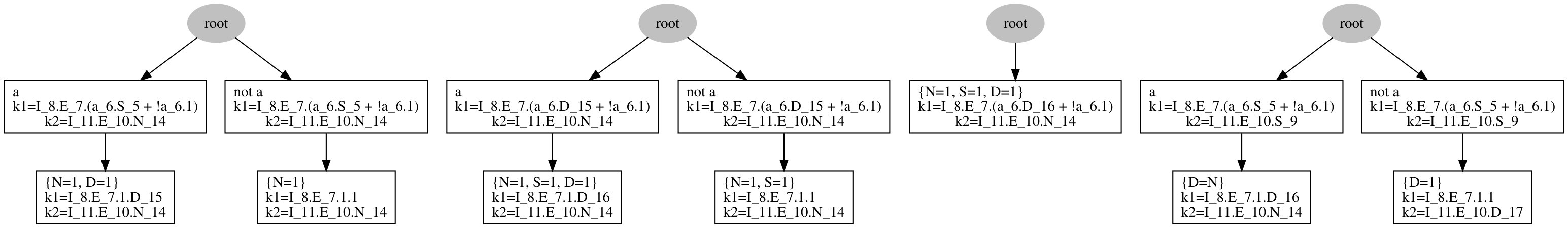 Figure 1
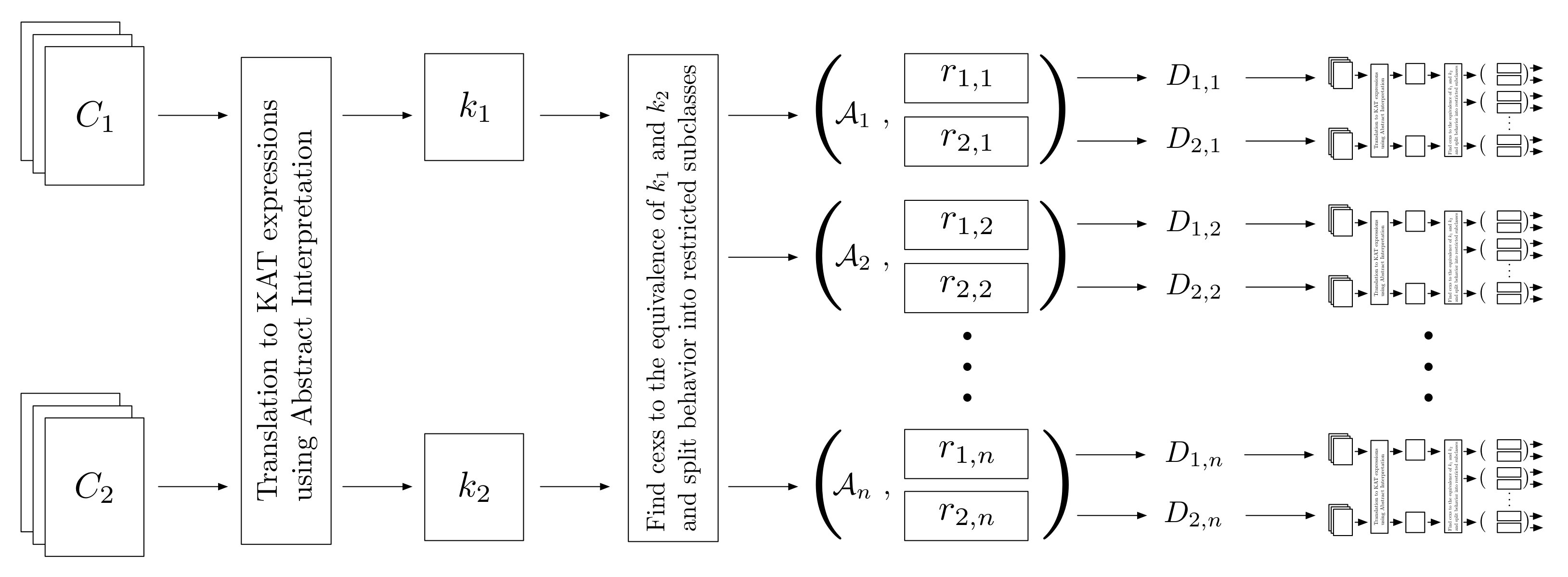 Figure 2
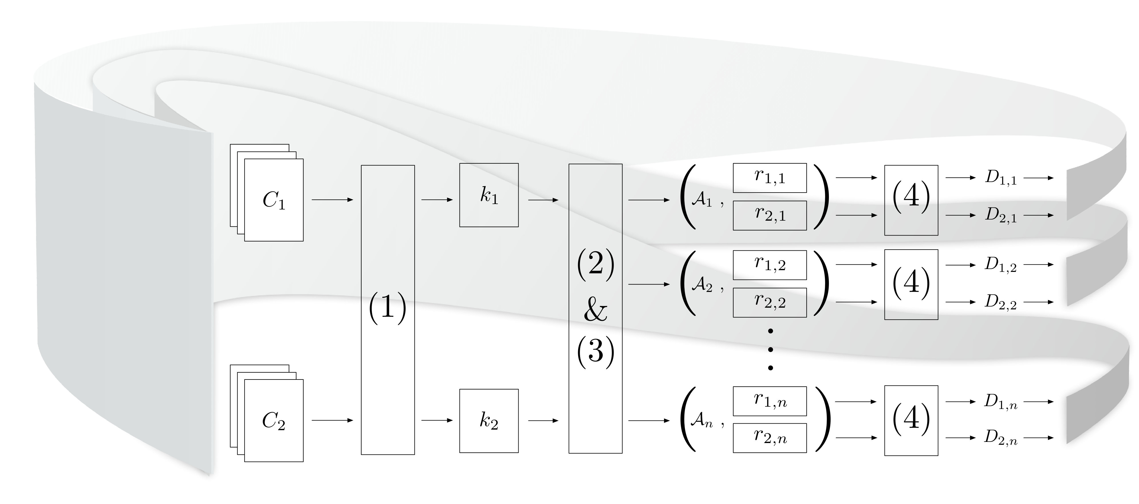 Figure 3
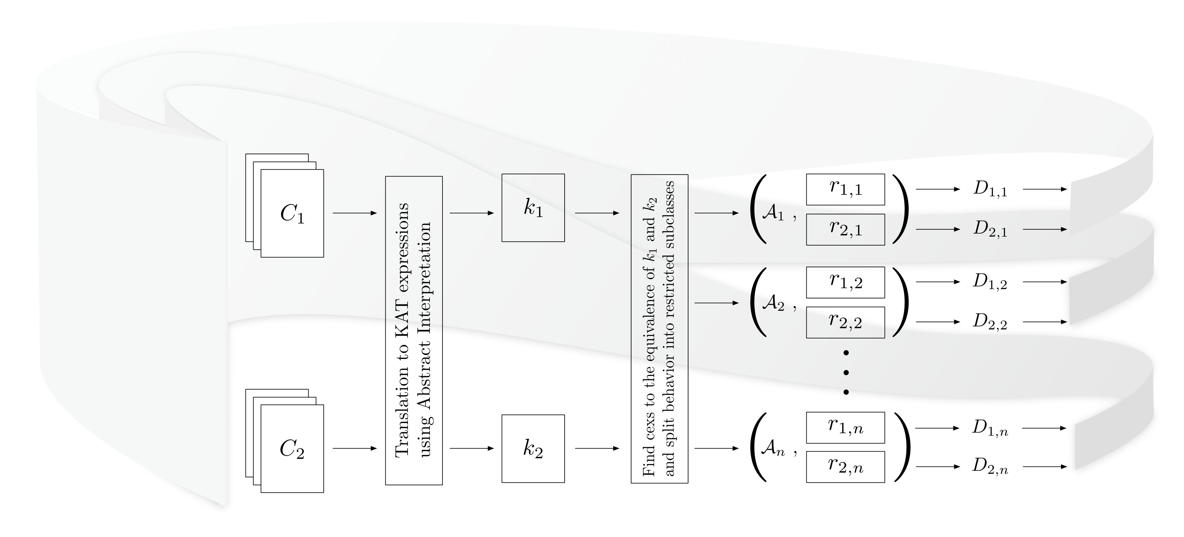 Figure 4
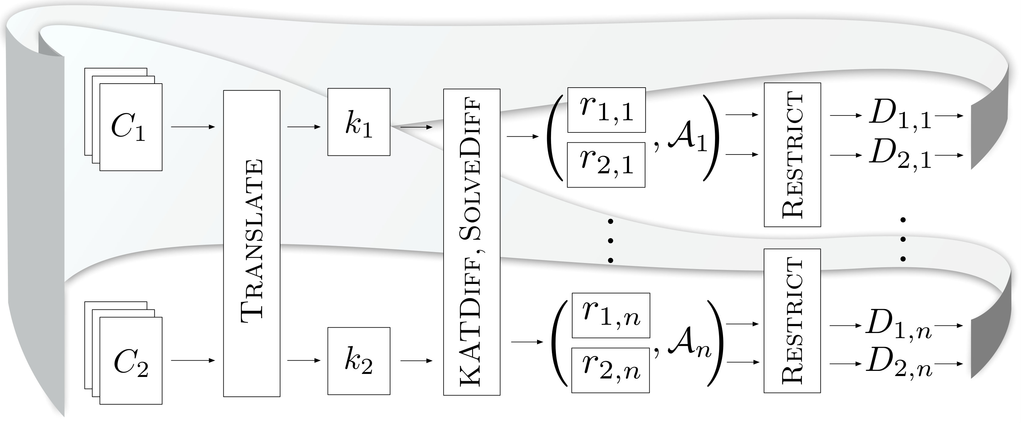 Figure 5
 Figure 6
Peer Reviews
No public reviews on file for this paper yet. If you reviewed it on a platform where reviews are public (OpenReview, ICLR, NeurIPS, ICML), you can paste yours below so the community can read it here.
Videos
No videos yet. Explain this paper in a talk, walkthrough, or lecture? Add one.
Taxonomy
TopicsSoftware Engineering Research · Software Testing and Debugging Techniques · Logic, programming, and type systems
numbers=none
1
Specification and Inference of
Trace Refinement Relations
Timos Antonopoulos
Yale University
,
Eric Koskinen
Stevens Institute of Technology
and
Ton-Chanh Le
Stevens Institute of Technology
(July 2018)
Abstract.
Modern software is constantly changing. Researchers and practitioners are increasingly aware that verification tools can be impactful if they embrace change through analyses that are compositional and span program versions. Reasoning about similarities and differences between programs goes back to Benton (Benton, 2004), who introduced state-based refinement relations, which were extended by Yang (Yang, 2007) and others (Gyori et al., 2017; Unno et al., 2017). However, to our knowledge, refinement relations have not been explored for traces: existing techniques, including bisimulation, cannot capture similarities/differences between how two programs behave over time.
We present a novel theory that allows one to perform compositional reasoning about the similarities/differences between how fragments of two different programs behave over time through the use of what we call trace-refinement relations. We take a reactive view of programs and found Kleene Algebra with Tests (KAT) (Kozen, 1997) to be a natural choice to describe traces since it permits algebraic reasoning and has built-in composition. Our theory involves a two-step semantic abstraction from programs to KAT, and then our trace refinement relations correlate behaviors by (i) categorizing program behaviors into trace classes through KAT intersection and (ii) correlating atomic events/conditions across programs with KAT hypotheses. We next describe a synthesis algorithm that iteratively constructs trace-refinement relations between two programs by exploring sub-partitions of their traces, iteratively abstracting them as KAT expressions, discovering relationships through a custom edit-distance algorithm, and applying strategies (i) and (ii) above. We have implemented this algorithm as Knotical, the first tool capable of synthesizing trace-refinement relations. It built from the ground up in OCaml, using Interproc (int, [n. d.]) and Symkat (sym, [n. d.]). We have demonstrated that useful relations can be efficiently generated across a suite of 37 benchmarks that include changing fragments of array programs, systems code, and web servers.
This work was supported in part by the National Science Foundation (NSF) award #1618542 and the Office of Naval Research (ONR) award #N000141712787.
††conference: ACM SIGPLAN Conference on Programming Languages; January 01–03, 2018; New York, NY, USA††journalyear: 2018††doi: ††copyright: none††doi: 0000001.0000001††ccs: Theory of computation Modal and temporal logics††ccs: Theory of computation Verification by model checking††ccs: Theory of computation Program verification††ccs: Theory of computation Abstract machines
1. Introduction
Modern software changes at a rapid pace. Software engineering practices, e.g. Agile, advocate a view that software is an evolutionary process, a series of source code edits that lead, slowly but surely, toward an improved system. Meanwhile, as these software systems grow, fragments of code are reused in increasingly many different contexts. To make matters worse, these contexts themselves may be changing, and code written under some assumptions today may be used under different ones tomorrow. With so many moving parts and adoption of formal methods an uphill battle, now more than ever, researchers and practitioners have found compositionality and reasoning across versions (O’Hearn, 2018; Logozzo et al., 2014). to be indispensable.
Changes can be exploited for good purposes: they offer a sort of informal specification, where programmers often view their new code in terms of how it has deviated from the existing code (i.e. a commit or patch), including the removal of bugs, addition of new features, performance improvements, etc. With compositional theories and tools, one can reuse previous analysis results for unchanged code, and combine them with new analyses of only the changing code fragment.
It is therefore a natural question to ask: how does a given program compare to , a modified version of ? If one is merely interested in knowing whether they are strictly equivalent (or whether is contained within ), this is a classical notion of concrete program refinement (Morgan, 1994) and includes compiler correctness and translation validation (Pnueli et al., 1998). Intuitively, concretely refines provided that, when executed from the same initial state, they both reach the same final state. Researchers have developed algorithms and tools (e.g. (Lahiri et al., 2012, 2013; Wood et al., 2017)) to check whether, say, two versions of a function return the same results. Similarly, bisimulation provides equivalence between how programs behave over time, perhaps accounting for different implementations.
Concrete refinement and bisimulation are not typically focused on how the programs differ, but simply whether or not they are equivalent. In his canonical 2004 work (Benton, 2004), Benton weakened classical refinement, allowing one to define equivalence relations over the state space, so that the two programs reach the same output equivalence relation when executed from states in a particular input equivalence relation. Such equivalences allow one to describe what differences over the states one does or does not care about, for example, focusing on important variables or ignoring scratch data. This strategy is compositional because one can correlate the output relation of one code region with the input relation of the next. Benton’s work was later extended by Yang (Yang, 2007) and others (Gyori et al., 2017; Unno et al., 2017).
Benton’s work focuses on state relations. To the best of our knowledge, no prior work has explored the question trace-oriented relations to express similarities/differences between the execution behaviors of and over time. Examples include whether two programs send/receive messages in the same order, follow the same allocation/release orders, or have certain I/O patterns. Encoding these kinds of properties in state relations with, e.g., history variables seems taxing, yet a trace approach would be appealing because it would be more granular and hopefully lead to more flexibility.
Toward trace refinement relations.
We take a reactive view of programs, treating their execution in terms of events, which can be suitably defined in terms of statements, function calls, I/O, etc. as needed. We considered a few options for characterizing traces. One choice would be a temporal logic such as LTL or CTL, perhaps using the LTL “chop” operator (Barringer et al., 1984) to support composition. We found Kleene Algebra with Tests (KAT) (Kozen, 1997) to be a natural choice for a few reasons. Briefly, KAT is an amalgamation of Kleene Algebra which (like regular expressions) has constructors for union +, concatenation , and star-iteration *, and boolean algebra which has boolean predicates and operations. KAT expressions consist of a combination of event symbols (herein denoted in uppercase: A, B, C) and boolean “test” symbols (herein denoted in lowercase: a, b, c). One can write KAT expressions that mix event symbols with boolean test symbols, e.g., . A KAT can be used as a helpful abstraction of simple abstract syntax trees. For example, the KAT expression models a program that is a multi-path loop, branching on b. In this way, programs can be abstracted into KAT expressions using a syntactic translation (Kozen, 1997, 2006) or, more generally using semantic translations, as we discuss later in this paper. Also, KAT is appealing because it supports algebraic reasoning, has a natural composition operator, allows hypothesis introduction, and there is existing tool support such as Symkat (Pous, 2015a). For KAT representations of programs, we can define an analog of concrete program refinement, called concrete KAT refinement (see Def. 4.2), but this is not enough to capture programs that have differences.
Contributions.
We present a novel theory of trace-refinement relations, which weaken both the notion of concrete KAT refinement as well as state refinement relations (Benton, 2004). Intuitively, the idea is to reason piece-wise and relate classes of program behaviors (traces) to classes of behaviors. We identify a class of traces by applying a trace restriction and, for that class, we identify an appropriate separate restriction that can be applied to . We also provide abstractions over individual events so that we can identify which atomic events in correspond to which atomic events in as well as which atomic events are unimportant. We treat a concrete program in terms of its traces by abstracting it—via an intermediate abstract program—to a KAT expression, denoted . A trace-refinement relation then characterizes the relationship between and in terms of their respective trace abstractions and . Specifically, each element of is a tuple embodying a trace class relationship: a restriction for , a restriction for , and atomic event/condition abstractions as a set of KAT hypotheses . The overall refinement condition is that, for each such triple, KAT inclusion holds over the programs restricted and abstracted trace-wise. Technically, we write to mean:
[TABLE]
Here denotes KAT inclusion (up to ), restriction is achieved through intersection, and the additional condition requires that accounts for all behaviors of . The latter requirement is not always enforced, as partial solutions are also useful. Our treatment based on restrictions, if applied to state-based relations, would be akin to taking the pre-relation to be disjunctive and considering each disjunct one at a time. Furthermore, notice there is no particular requirement on the relationship between and within a tuple, affording flexibility in how to relate the corresponding classes. Finally, we have shown that our trace-refinement relations are composable (Thm. 4.5), permitting an analysis of one pair of program fragments to be reused in many contexts and when the program is further changed.
The second part of our work introduces a novel algorithm that is able to synthesize a trace-refinement relation , given input programs and , such that . Overall, our search algorithm constructs triples, by looking for restrictions that can be placed by , on and relaxing their behavior with new hypotheses . Each stage of our algorithm is a candidate tuple of trace classes—that may need further restriction—and we proceed as follows. First, we iteratively synthesize a two-step semantic abstraction from a program (and ) to a KAT expression (and ). This semantic translation goes beyond the syntactic -to- translation of Kozen (Kozen, 1997), expressing restrictions (via assume) and accounting for paths becoming infeasible. Second, we check whether is included in using KAT reasoning, returning a counterexample string if not. Third, we use a custom edit-distance algorithm on such counterexamples to find relationships between cross-program trace classes, with a scoring scheme to correlate program behaviors. Fourth, we employ case-analysis on branching in and , in circumstances where the branching in one program prevents immediate inclusion in the other. This leads us to introduce more restrictions which—unlike (Benton, 2004; Yang, 2007; Gyori et al., 2017; Unno et al., 2017)—are not required to be of the initial state, but rather may appear at program locations anywhere in the program. When we are unable to continue refinement through case-analysis, we introduce KAT hypotheses that either treat unimportant events (e.g. logging) as skip, or else equate similar events. Finally, we construct increasingly restricted trace classes used in subsequent iterations of the algorithm.
The goal of our work is to build foundations for compositional trace-based reasoning. To this end, we generate trace-refinement relations to capture the multitude of conditions and ways in which one code region can refine another region , in order to produce results that are reusable. Additionally, synthesized trace refinement relations can also be used by experts. Like a syntactic diffing tool, the relations can guide them to understand how code has changed.
We have implemented our algorithm in a new tool called Knotical, that operates on an input pair of C-like programs and synthesizes trace refinement relations. Knotical is built from the ground up, in OCaml using Interproc (int, [n. d.]) for abstract interpretation, Symkat to generate KAT counter examples (sym, [n. d.]; Pous, 2015a), and our own edit distance algorithm.
We have evaluated our tool on a collection of 37 benchmark examples that we have built (Apx. C). Almost all examples necessitate trace refinement relations that cannot be expressed using concrete refinement or other prior techniques. The examples range from those designed to exercise the various aspects of our approach (restriction, hypotheses, edit distance, etc.), to broader examples including user I/O, array access patterns, and reactive web servers (e.g. thttpd (Poskanzer, [n. d.]) and merecat (Nilsson, [n. d.])). Our evaluation demonstrates that interesting and precise trace refinement relations can be discovered.
Summary.
We make the following contributions:
- •
A theory of trace-refinement relations, going beyond prior state refinement relations. (Sec. 4)
- •
A proof of composition. (Thm. 4.5)
- •
A novel synthesis algorithm that iteratively constructs trace-refinement relations. (Sec. 5)
- •
A proof of soundness. (Thm. 5.1)
- •
The first tool for trace refinement relations. (Sec. 5-7)
- •
A customized edit-distance algorithm for scoring and finding alignments between programs. (Sec. 6)
- •
A collection of benchmarks and experimental validation, demonstrating viability. (Sec. 7)
Related work.
To our knowledge, we are the first to generalize Benton-style refinement (Benton, 2004; Yang, 2007) to trace relationships. Bouajjani *et al. *(Bouajjani et al., 2017) have focused on concurrent loop-free programs. Their notion of refinement is not quite based on “traces” in the sense that we describe herein, but rather on graphs over the reads-from relation and program order. More distantly related are bisimulations, hyper temporal logics (Clarkson et al., 2014) and self-composition (Barthe et al., 2004; Terauchi and Aiken, 2005). (See Sec. 8)
Limitations.
We developed a theory for trace refinement relations and, while KAT has worked well, it has also meant that we were restricted to terminating programs. We leave possibly non-terminating programs to future work. Our implementation was also limited in the number of symbols due to Symkat (sym, [n. d.])’s use of char to represent symbols.
2. Overview
Consider the two programs in Fig. 1, inspired by the Merecat project (Nilsson, [n. d.]) which enhanced the thttpd web server (Poskanzer, [n. d.]) to support SSL connections. We are interested in knowing how the the new program compares to the previous, both of which involve typical web server behavior: alternately receives a request and sends a response. This is illustrated by the two program fragments and . The programs involve some differences, perhaps arising from changes/edits that were made to . There are still similarities: both programs involve a loop that iterates over x, recving messages and possibly sending responses. On the other hand, only performs a log when it recvs an m such that , and it additionally performs an authorization check on m. In addition, only performs logs when the flag l is enabled.
2.1. Relating the programs’ behavior over time
We take a reactive view of programs, considering not only the programs’ local stack/heap state, but also the programs’ I/O side-effects. For simplicity in this paper we will work with stack variables and events shown as function calls (denoted recv, log, etc.) but our work generalizes to heap structures.
We would like to express similarities in how the programs behave over time, such as alternation between send and recv. We would like a theory to also tolerate the differences between how the programs behave over time, such as the recv/send behavior in versus the recv/check/send behavior in . Intuitively, the theory we develop will need some way of expressing restrictions that can be placed on one program (e.g. auth is always greater than 0 in ) so that its traces are included in the other (e.g. log-free traces of ), as well as to provide abstractions that relate an event in one program (e.g. the send event in ) to an analogous event in the other (e.g. send in ).
Expressing properties of the way a program behaves over time motivates the need for a suitable trace-oriented relational logic (as opposed to state relations (Benton, 2004; Yang, 2007; Gyori et al., 2017; Unno et al., 2017)). As discussed in Sec. 1, we found that Kleene Algebra with Tests (KAT) was a natural choice (Kozen, 1997) for a few reasons, including that the KAT constructors naturally abstract program entities. Our theory involves an abstraction from concrete programs , via abstract programs to a representation as KAT expressions , respectively (Sec. 4.1).
The terms of a KAT expression are event symbols or boolean test symbols. We introduce (uppercase) event symbols for program statements such as “” for recv and (lowercase) boolean test symbols for the integer expressions above such as “” for x>0. (For ease of reading, we use subscripts to indicate which program expressions correspond to the symbol.) Thus, the behaviors of programs and in Fig. 1 can be represented, respectively, as:
[TABLE]
where “1” is the identity symbol in KAT, akin to skip in programs. Note that composition binds tighter than union , and we use overline (e.g. ) to indicate negation. The above KAT symbols represent program statements, but we use KAT symbols more generally as semantic entities.
Trace-refinement relations.
With KAT representations of programs, it is straight-forward to define concrete KAT refinement (Def. 4.2 for programs that are equivalent. However, not all behaviors of are contained within (such as some logging in ) and vice-versa (authorization failures in ) and so KAT refinement does not hold for Fig. 1. Nonetheless, we may still be interested in which behaviors of are in and how one might correlate events in with . We may want to describe how both programs have a substantially similar recv/send relationship. Imagine that we could somehow focus on the executions of in which auth was always greater than 0, somehow focus on the executions of that had no log events (when l was always false), and finally on the executions of both programs where they recv valid messages and thus . In that case, the programs would have the following more restricted behaviors, represented as the following restricted KAT expressions:
[TABLE]
The above equations are just classes of trace behaviors of and , respectively, with denoting KAT inclusion. If we could now further somehow ignore the event, the above KAT expressions are equivalent. (In this case they are syntactically equivalent, but they could also be semantically equivalent.) Finding this correlation takes care of some behaviors of . Doing this for all behaviors of leads us to our trace-oriented notion of refinement relations.
We formalize this kind of reasoning into a weak (as opposed to concrete) and compositional notion of refinement based on what we call trace-refinement relations. We consider one class of traces of at a time like we did above in Eqns. 1 and 2. We translate programs into KAT expressions and then reason abstractly about traces of by considering its corresponding KAT expression and focus on particular behaviors by restricting behaviors—also described as another KAT expression —with intersection: . For this restricted behavior of , it is then often helpful to restrict (which corresponds to ) with a perhaps rather unrelated . Then we can ask whether equivalence holds between and . Returning to the running example, we can consider the class of traces of in which auth is always greater than 0 by letting
[TABLE]
where Any is shorthand for the disjunction of all event symbols in the KAT at hand. This restriction allows behaviors of the program where after any event, both and . We can use this restriction to focus on . Similarly we can restrict to the classes of traces that do not involve logging by letting
[TABLE]
requiring that holds on every iteration of the loop. With these restrictions in place, we get Eqns 1 and 2 above.
In some cases, we can witness classes of traces in that are in simply with a pair of restrictions. However, restrictions are not the only way that we relate to . Looking at Eqns 1 and 2, there is still the discrepancy that the event occurs in but not . Since we are already focused on a case where auth is always greater than 0, the event is not so important. We can ignore such unimportant events by introducing additional hypotheses into the KAT. In this case, we can introduce the hypothesis “,” and we finally have the KAT relationship . Our choice of working with KAT enables us to exploit algebraic reasoning and so we can introduce hypotheses for other purposes too. It is often convenient to let syntactically identical statements between and use the same KAT symbol. In other cases, we may prefer not to, but we can introduce KAT hypotheses to instead selectively relate statements.
Putting it all together.
As discussed so far, we have only considered one class of traces and there are of course many others. Ultimately, we will collect a set , each triple considering different cases. Overall, we use the notation to mean that holds of each triple and that if we union over the first projection of , we have taken care of every possible behavior of . Notice that for “weak” completeness we could always add a triple where maps every single symbol to 1 (skip). The goal is instead to generate useful and precise trace-refinement relations. To this end, our algorithm and implementation favor searching for complex restrictions and resort to hypotheses only when necessary.
To the best of our knowledge, one cannot describe these kinds of trace-based refinement relations in prior works such as Benton (Benton, 2004) and bisimulation (at least not without extraordinary effort to represent trace behavior with complicated ghost variables). Nonetheless, there are many intuitive trace-based properties that one would like to express along the lines of the new program alternately receives and sends messages like the original, the new program additionally performs an authorization check after each receive, and so on.
Remark: Path Sensitivity. KAT has facilities to express many well-known tricks for increasing path sensitivity such as loop unrolling, trace partitioning (Mauborgne and Rival, 2005), control-flow refinement (Gulwani et al., 2009). For lack of space, we omit examples such as alignments between different loop iterations.
2.2. Composition, Contexts, Spanning Versions
So far we have discussed reasoning about a change from to , while the context remains fixed. But what about the context of ? A single fragment can be used in many different contexts within a large program. Thus, when is changed to , there is benefit to performing a single analysis that considers all possible contexts, rather than considering how and relate in each context (O’Hearn, 2018). This approach also allows us to cope with the fact that the context itself may change. Consider, for example, programs:
[TABLE]
In these programs, we need to know how and relate in a context of boolean symbol b and how they may impact boolean symbol g. If this were the only context we were concerned about, we could focus on search for refinement relations to those that assume b. However, what if the program is then changed to , where b is no longer in the context, but m is? If we are context agnostic in our analysis in our -vs- analysis then we can reuse refinement relations for reasoning about -vs-.
Returning to Fig. 1, fragments and may be used in different contexts. Perhaps in one context it is important that all failed connections are logged and we want to ensure a change from to preserves this property. In that case we need a refinement relation that does not ignore log events, and assume that the context of ensures . Formally, we would have the tuple
[TABLE]
This restricts to traces of where logging is enabled and all connections fail and restricts traces of to those where all connections fail. Moreover, we require a set of hypotheses which does not imply that .
In a different context, other relations would be useful. As noted earlier, this example comes from a change that added SSL support to thttpd (Poskanzer, [n. d.]). Therefore, we may wish to have a refinement relation, specifying that as long as all messages are authenticated in , then it behaves the same as . Our theory allows one to express this relationship written, formally as:
[TABLE]
Here, is unrestricted, is focused only on executions that are authorized, and we use a set of hypotheses that ignores all log events and ignores the check event in .
It is not hard to see that our formalism can capture other more complicated contexts, such as an outer loop. More broadly, encompasing all of KAT, we have proved that our trace-refinement relations are compositional (Thm. 4.5), allowing us to reason about the overall trace-refinement, by considering pairs of program segments at a time.
2.3. Automation
From to and back.
Before we present our main algorithm, we need to translate back and forth between a program and its corresponding KAT expression . The former lets us learn fine-grained details about the behavior of the program, while the latter lets us perform coarse-grained cross-program comparisons. To get from , we exploit program semantics to obtain precise KAT expressions, e.g. excluding infeasible paths. Technically, we work with an (iteratively refined) two-step abstraction function that takes concrete states, via abstract states, to symbols in the KAT boolean subalgebra, using a procedure called (see Sec. 4.1). Our abstraction is not a one-way process: our refinement search (discussed below) involves discovering various classes of traces of , each expressed as a restriction . For example, we may consider traces of in which auth in Line 1 is always positive. Our algorithm discovers the restriction in Eqn. 3, and uses a subprocedure to instrument these restrictions via a source code transformation. We now need to translate this back into the program so that we can explore more fine-grained behaviors of with help from abstract interpretation. This is denoted and our implementation represents these restrictions via a source code transformation, using a form of a product program in which we instrument assume statements. As our algorithm continues to search for more fine-grained classes of traces where refinement holds, it may iteratively instrument more assumptions and continue to refine the abstraction (maintaining a monotonicity constraint).
Overall algorithm:
The above is a depiction of our overall algorithm (Sec. 5) that synthesizes trace-refinement relations by attempting to discover increasingly granular trace classes of that are included in trace classes of . Each such partial solution is a triple such that (Def. 4.4), where corresponds to and to .
At the high level, each iteration of the algorithm is a recursive call (Synth), where we are exploring a region of the solution space where has possibly been restricted, has possibly been restricted and a collection of KAT hypotheses are in use. Moreover, we have a current abstraction from programs to . Each iteration of our algorithm proceeds by calculating the aforementioned KAT abstractions and of the (possibly already restricted) programs (Translate). Next, we consider whether is included in or is equivalent to , under the current set of hypotheses (KATdiff). To check this refinement, we build on the recent work of Pous (Pous, 2015a), using his tool Symkat (sym, [n. d.]). If this refinement holds, then the algorithm returns this triple as a solution that may be assembled with others into a complete solution by previous calls to Synth. Alternatively, if the inclusion/equivalence does not hold, we employ a sub-procedure (SolveDiff) to decide, based on the counterexamples and the overall KAT expressions, whether to (i) introduce restrictions and/or (ii) introduce hypotheses . In Secs. 5 and 6 we discuss how the sub-procedure employs a custom edit distance algorithm for this purpose. Finally, the restrictions and are instrumented back into the programs (Restrict), to produce new programs and that are considered recursively. We have proved that our algorithm for generating trace-refinement relations is sound (Thm. 5.1). Weak completeness is less interesting because any partial solution can easily be made a complete solution through aggressive use of hypotheses. We note that we do not expect from our algorithm to be able to generate every possible solution. Hence, we are more interested in generating precise and useful trace-refinement relations.
2.4. The Knotical Tool
We have developed a prototype tool Knotical that implements our algorithms and is the first tool capable of synthesizing trace-refinement relations. Our tool is built from the ground up written in OCaml and uses Interproc(int, [n. d.]) for abstract interpretation and Symkat (Pous, 2015a) for symbolically checking KAT expression equalities and inclusion.
Fig. 2 illustrates one of the 75 solutions found by Knotical when run on the example in Fig. 1. The synthesized trace refinement relation has five tuples. This output illustrates the restrictions using the notation “” meaning, for example, that we instrument an assume(auth>0) on line 1 of . Notice that Knotical has considered various case splits, based on these three boolean conditions. It begins with the conditions in the left-hand side () and needs to discover at least one solution in for each case. When auth>0, Knotical introduces hypotheses to ignore log events in either program and the check event in . Otherwise the log event does not occur in so it needn’t be ignored.
Edit-distance for refinement.
During the algorithm, when considering whether the current refines , Symkat may find that it doesn’t and return a counterexample of a string that is in but not (and , vice-versa). Returning to the running example, such a pair might be and . These counterexamples give us information as to how and diverge. Our algorithm departs from a traditional counterexample-guided approach and instead is able to consider not only the entirety of counterexample strings and , but also the KAT expressions and , in order to find a better correlation between the two. It is easy for a human reader to see that the relationship between and fits better, when the * expression in is correlated with the * expression in . To this end, we developed a custom edit-distance algorithm (Bille, 2005) (see Sec. 6).
Evaluation.
We created a series of 37 benchmarks for most of which, trace-based refinement relations cannot be expressed in prior formalisms (Sec. 7). On most benchmarks, our tool was able to generate a non-trivial trace-refinement relation in seconds or fractions of a second.
3. Preliminaries
Strings, Sets, Composition, Programs
A string over an alphabet is a sequence of symbols , for . Given sets , a set , and an element we denote with the projection of to its -th element in . We abuse notation, denoting as the set .
We assume a set of (essentially imperative) programs operating on a set of states. We assume a distinguished “error state” . A configuration is a pair , where is a program and a state; we write for the set of all configurations. We assume a binary relation capturing the “big step”, nondeterministic operational semantics of our programs; means that executing program in initial state can result in the final state .
Kleene Algebra with Tests.
We use KAT (Kozen, 1997) to represent classes of traces within a program. A Kleene Algebra with Tests is a two-sorted structure , where is a Kleene algebra, is a Boolean algebra, and is a sub-algebra of . We distinguish between two sets of symbols: set P for primitive actions, and set B for primitive tests. The grammar of boolean test expressions is: and we define the grammar KExp of KAT expressions as:
[TABLE]
The free Kleene algebra with tests over , is obtained by quotienting BExp with the axioms of Boolean algebras, and KExp with the axioms of Kleene Algebra. For , we write if , and all Kleene Algebras with Tests we consider here are -continuous, where any elements in , satisfy the axiom ((Kozen, 1990)). By convention we use lower case letters for test symbols and upper case letters for actions. We may also abuse notation, writing program conditions and statements rather than boolean symbols and action symbols (in which case we implicity create symbols for each). For Fig. 1 booleans include , actions include , and .
Definition 3.1 (Intersection).
Given a KAT and two of its elements and we define to be equal to , where is the set of all elements in such that and .111Notice that for any two KAT expressions and over a KAT , for , there is a finite number of elements , for such that . Since we never start with a KAT expression as an infinite disjunction in what follows, any time we talk about the intersection of two KAT expressions as a disjunction of KAT elements, we will refer to such a finite disjunction.
For KAT expressions and , and a set of hypotheses , we write if and . Similarly, we write if or . Finally, for two KATs and , we denote with the smallest KAT that contains both and . Finally, when we refer to strings we mean KAT strings, which are KAT expressions where only the concatenation operation is used.
Program Refinement.
Program refinement is a classical concept (Morgan, 1994) and can be formulated in different ways, depending on the context. Often, the usual notion of refinement is too concrete because it does not consider the context in which and are used. Benton (Benton, 2004) introduced a weaker notion of refinement, parameterized by an input relation between the states of the two programs as well as an output relation. We call this an interface, which is an equivalence relation on the set of states and defined as follows:
Definition 3.2.
For interfaces and programs , we say refines w.r.t. , written , if the following two conditions are met, for all states such that :
- (1)
if , then ; 2. (2)
if , then either there exists such that and , or else .
We say that (concretely) refines , written , when where id is the identity relation.222Benton used the notation whereas we use notation by James Brotherston (personal communication)
Yang (Yang, 2007) extended Benton’s work to express relational heap properties using a variant of Separation Logic (O’Hearn et al., 2001).
4. KAT Representations and Refinements
In this section we discuss a two-step semantic abstraction (Sec. 4.1), trace refinement and trace-refinement relations (Sec. 4.2), and composition results (Sec. 4.3).
4.1. Abstracting programs into KAT expressions
We describe how to abstract a while-style program to a KAT expression over a KAT . We parameterize such a translation by an abstraction used for both abstracting concrete states of the program to abstract states, as well as the latter to elements of the boolean subalgebra of . More concretely, given a program over a set of states , we define to be a tuple , where is a KAT, is a set of abstract states, is a mapping from to corresponding to the program abstraction given by the abstract interpretation, and is a mapping from to , the boolean subalgebra of . Additionally, we require that for any , there is a set of states such that . When and are clear from the context, we write .
With such an abstraction as a parameter, we say a translation from to a KAT expression is valid (resp. strongly valid), if for any states , only if (resp. if and only if) . We assume a procedure that returns and the translation from to is valid (Sec. 5 for an implementation). Finally, we will (Sec. 5) iteratively construct abstractions and thus need the following notion of refinement over abstractions:
Definition 4.1 (Refining abstractions).
For two abstractions and over the same set of concrete states , we say that refines , and write it as , if is a subalgebra of and for any state , .
Let and be two abstractions, both refining an abstraction with Boolean algebra . By we denote the function from to , that maps a state to . Further, we define to be the function from to that maps a tuple to in . The combined abstraction of and , written , is defined to be the abstraction .
4.2. KAT refinements
With abstractions from programs to KAT expressions in hand, we now first define concrete KAT refinement, and then our notion of trace-refinement relations (Def. 4.4).
Definition 4.2 (Concrete KAT refinement).
Let and be two KAT expressions over . We say that concretely refines , and denote it by , if for any :
- (1)
implies , 2. (2)
implies , or .
The following relates concrete trace refinement, via abstraction, back to concrete program refinement (See Apx. A).
Theorem 4.3.
Let and be two programs, and let and be the two KAT expressions obtained from a strongly valid translation of the two programs respectively, under some abstraction . Then it holds that if and only if .
We now weaken concrete KAT refinement, presenting trace-refinement relations. Intuitively, the idea is to reason piece-wise, considering classes of traces within and, for each, correlating them with a corresponding trace class in , with the help of KAT hypotheses. Note that, for some element of a KAT , we say a set of elements partitions , if .
Definition 4.4 (Trace Refinement Relations).
Let be a KAT, let be a class of hypotheses over , and let be a relation over . Given two KAT elements and of , we say that refines , with respect to , denoted by , if and,
[TABLE]
We also consider trace equivalence relations, slightly adapting Def. 4.4 to use equivalence (), rather than inclusion (), as well as requiring that both partitions and partitions .
As discussed in Sec. 2, intuitively each triple in a trace-refinement relation identifies restrictions on and , as well as KAT hypotheses that allow us to align the trace classes with ones in . In the example from Sec. 2.1, we gave examples of an that excluded logging by forcing to hold at each iteration of the loop.
Remark 4.1.
As trace-refinement is a weakening of concrete refinement, it is natural that two KAT expressions and may be such that refines , but does not concretely refine it. For any two expressions and , the singleton set containing only the tuple , where is a set of hypotheses that equates all actions to and all boolean variables to [math] is a trivial solution to trace-refinement between and .
Finally, we overload the KAT refinement definition to be used on programs themselves, when the abstraction is clear from the context. Thus, for two programs and , and a trace-refinement relation , we may write to mean that .
Classes of hypotheses.
For this work, we will explore the effect of just a few types of classes of hypotheses. In general, checking equality of KAT expressions under arbitrary additional hypotheses, can be undecidable ((Kozen, 1996)). Because of that, and guided by the limitations imposed by certain libraries we use in our implementation (Symkat), we focus on the following types of hypotheses when and : (i) to ignore certain actions: , (ii) to fix the valuation of certain booleans: or , (iii) to express commutativity of actions against tests: (currently not used in our implementation) and (iv) to relate single elements: or .
4.3. Composition
Given trace-refinement relations and , we define their composition to be the trace-refinement relation . Similarly, we define disjunction to be the trace-refinement relation . Finally, for , we define to be .
Thm. 4.5 below allows us to reason about individual fragments of KAT expressions, and combine the analyses into a result that holds overall. We can do so by building trace-refinement relations in a bottom-up fashion, capturing larger and larger fragments of those KAT expressions, guided by their structure. (See Apx. A)
Theorem 4.5.
Suppose and are KAT expressions. Let and be trace-refinement relations, such that and . Then , , , and .
As a simple corollary we can always extend a trace-refinement relation corresponding to a pair of KAT expressions, to one corresponding to a pair of KAT expressions obtained from the former by enclosing them into any common context.
Corollary 4.6.
Given any KAT expressions and , and trace-refinement relation such that , it holds that , where is the set .
Finally, we present a transitivity result, stating how we can extend two trace-refinement relations to achieve it. Let and be two trace-refinement relations, such that for any tuple in , there is a tuple in , such that . For such trace-refinement relations, we define their transitive trace-refinement relation to be the one containing the tuples . We denote such a trace-refinement relation by .
Theorem 4.7.
For any elements and in a KAT , and any trace-refinement relations , , if and , and is defined, then .
5. Automation
Our overall algorithm is given in Fig. 3. The input to our algorithm are programs provided, for example, in a C-like source format and parsed into ASTs. Our algorithm returns trace-refinement relations for , and is parametric as to whether the relations are for equivalence versus inclusion. Technically, it returns a finite set from which the trace refinement relation can be constructed by unifying to a common abstraction .
Our main function Synth uses several sub-components discussed below. At the high level, it begins by using Translate, analyzing and using an iteratively constructed abstraction to obtain the KAT expression (similar for ), per Sec. 4.1. The algorithm then checks for KAT equivalence or inclusion between and with KATdiff. If no counterexamples are found, KATdiff returns and , together with the current set of hypotheses as a solution. On the other hand, if KATdiff does find counterexamples, they are fed into SolveDiff, which examines them along with the KAT expressions to determine what restrictions and/or hypotheses could be employed to subdivide the search space into trace classes for which we hope further refinements can be discovered. SolveDiff returns this decision, given as a list of triples. Then Restrict is used to construct increasingly restricted versions of the input programs and and new abstractions . These are then are considered recursively by Synth.
5.1. Sub-procedures
We now define and discuss the sub-procedures used by Synth. We also discuss the implementation (and limitations) of these subcomponents. As noted, the overall algorithm is parameterized by whether we are looking for solutions to equivalence (), or simply to inclusion (). The functionality of the sub-procedures is largely the same for the two cases.
: As described in Sec. 4.1, this sub-procedure takes as input a program and abstraction , and returns a KAT expression in such that implies that . In the implementation, Interproc populates the locations of the program with invariants according to abstraction . This is then used in converting the abstract program into a KAT expression in that covers its behavior. Semantic information is exploited where paths of the program are determined to be infeasible. For example, consider the simple instrumented program
asm(d==0); c=d; if (c==0) execB() else execD(); The standard syntactic translation (Kozen, 1997) alone, would produce the expression In our case, Interproc determines that c==0 is always true under the instrumented asm(d==0) and the program is instead converted to the simpler expression .
: Given two KAT expressions and hypotheses , KATdiff returns cexs, which is a set of KAT expressions with and possibly (depending on whether we seek equivalence or inclusion). We assume this sub-procedure to be sound and complete. If cexs is empty, then the two input KAT expressions and are such that (or ). Our implementation uses Symkat (sym, [n. d.]), which only obtains a singleton set cexs, and is thus either (i) a single string in when we seek inclusion or (ii) a pair of strings , with in and in , when we seek equivalence. If and , then the string is included in but not in , and thus in .
: This procedure takes KAT expressions and , a set of hypotheses, and the set of counterexamples cexs above. It returns a set of tuples , each called a restriction. Restrictions has the property that partitions , ensuring that we have completely covered all traces. Furthermore, in the interest of progress, we also assume that each counterexample in cexs is not a counterexample for , or even for depending on whether equivalence is considered instead of inclusion. In our implementation, we apply a customized edit-distance algorithm discussed in Sec. 6, which returns a set of transformations that can be applied to two KAT strings and to make them equivalent. These transformations are in the form of removing alphabet symbols from the strings at particular locations, or replacing some symbol with another. From these transformations, SolveDiff constructs a list of restrictions to be applied on the input programs of the form , where and are KAT expressions, and is a set of hypotheses.
When the edit-distance algorithm asks for the removal of an alphabet symbol from, say, string , we consider two cases, depending on whether the symbol corresponds to a boolean condition or not. If so, the KAT expression corresponding to this transformation is essentially obtained by adding a hypothesis inserting the valuation of the boolean variable, in the given KAT expression . Since we want these restrictions to cover all behaviors of the input programs, we also consider the negation of that valuation. As such, at least two restrictions are considered, namely and , such that and cover . On the other hand, when the removal of an event is required, a hypothesis of the form is added to the set of hypotheses.
obtains new programs from previous ones, using restrictions from SolveDiff. Given programs , KAT restrictions , a set of hypotheses and current abstraction , this sub-procedure returns a tuple , where are the new programs and is a new abstraction that refines , such that, for , , but . In other words, the KAT expression obtained from the new program under the new refined abstraction , is included in the KAT expression from the original program under the old abstraction using the restriction , but at the same time, if we used the new abstraction to translate the program under the restriction , into a KAT expression we would obtain the same as by just translating under the new abstraction. Our implementation restricts programs by instrumenting assume statements on appropriate lines of code. For example, for a program we can implement restriction with an assume(l==true) instrumented immediately inside the body of the corresponding while loop. This can be seen in the output of our tool shown in Fig. 2.
5.2. Formal Guarantees
The key challenge is soundness, even under the sub-procedure assumptions noted above, and the proof is in Apx. A.1..
Theorem 5.1 (Soundness).
For all , and abstractions , let , let be the common abstraction of and let and . Then .
Weak completeness is easier because, as per Remark 4.1, trivial solutions can be constructed. So we are more interested in generating increasingly precise solutions. For progress, as long as the sub-procedure SolveDiff returns restrictions that handle the counterexamples returned by KATdiff, then these counterexamples will not be seen again in the recursive steps that follow.
6. Edit-distance on expressions and strings
Our main algorithm depends on SolveDiff to examine a pair of KAT expressions , a set of hypotheses , as well as counterexamples to their equivalence, and determine appropriate restrictions and additional hypotheses that could be used to further search for trace classes of that are contained in , up to hypotheses . To achieve this, SolveDiff tries to identify the differences between the KAT expressions and , or between their string-based counterexamples, and attempts to find useful restrictions of least impact, to apply to the two input programs. As such, we implemented a sub-procedure Distance, that takes as inputs two KAT strings and , or two KAT expressions and , and returns a list of scored transformations to be applied on the two strings (or KAT expressions) in order to make them equivalent. In our implementation we use the custom edit-distance algorithm only on counterexample strings, and in Apx B.1, we discuss how the global edit-distance for general KAT expressions can help in conjunction with the composition results of Section 4.3. The edit-distance on such KAT expressions has to handle the structure of the expressions, and is naturally more involved than the linear one on strings. (The former is more similar to trees (Bille, 2005).) The idea behind the sub-procedure Distance is similar to edit-distance algorithms in the literature for comparing two strings/trees/graphs (Bille, 2005). These edit-distance algorithms, return a sequence of usually simple single-symbol transformations that are classified as symbol removals, insertions, and replacements, that equate the two input strings when they are applied on them.
We had to customize edit distance for our purposes of cross-program correlation. We thought that inserting a symbol in one of the two strings or KAT expressions, is less natural than removing another one from the other string or expression, and encode such insertions in one string as removals from the other. Therefore we employ just removal and replacement transformations on the two inputs:
- •
: Returns a new string obtained from with the symbol removed,
- •
: Returns a new string obtained from with the symbol replaced with the symbol .
Note that each copy of each symbol in the string is uniquely labeled, and the transformations above speak about these labeled symbols, making the order in which the transformations are applied irrelevant. Moreover, in our experience, certain transformations have more impact, or are in some way heavier than others. As such, we attempt to score them, and use the score of each individual transformation to ultimately score the whole sequence of transformations. For example, replacing an event symbol in some string with another symbol , is certainly a transformation that is semantically more involved than simply setting a boolean symbol to . The full algorithm for edit-distance can be found in Appendix B of the supplemental material.
Example 6.1.
Consider the two input strings and . Running the procedure Distance on and , will return the pair , where is the sequence of transformations and the score , where is the cost of replacing one symbol with another of same type, and is the cost of removing a symbol from one of the input strings. With this sequence of transformations, both strings become equal to .
The sequence of transformations returned by Distance is converted into the one SolveDiff returns, as follows, for action symbols and boolean symbols.
- •
: add a new hypothesis
- •
: perform case analysis and include two tuples of restrictions, resp. corresponding to setting to and setting to
- •
: add a new hypothesis
- •
: add a new hypothesis
7. Evaluation
Implementation
We have realized our algorithm in a prototype tool called Knotical. Our tool is written in OCaml, using Interproc as an abstract interpreter (int, [n. d.]), and Symkat as a symbolic solver for KAT equalities (Pous, 2015a; sym, [n. d.]). We have described implementation choices made for the tool’s subcomponents in Section 5.1. Knotical generates multiple solutions, internally represented in the form of trees. During the KATdiff and SolveDiff steps of the algorithm, multiple choices can be made and each solution tree corresponds to a particular set of choices. Branching in a solution tree corresponds to the different restrictions applied and their complement, as a result of performing case analysis on a particular condition. Often the solution trees (or subtrees) are partial, in the sense that the different restrictions applied to the programs, when taken together do not cover all behaviors of the input programs. Partial solutions can readily be converted to complete ones (See Remark 4.1)
Benchmarks.
We have evaluated our approach by applying our tool to a collection of 37 new benchmarks. Each benchmark includes two program fragments denoted and . They can be found in Appendix C of the supplemental materials. Broadly speaking, our benchmarks categorized as: (0*.c) – Program pairs that exercise various technical aspects of our algorithm, such as cases where refinement is trivial, concrete refinement holds, refinement can be achieved entirely from case-splits, and where refinement can only be achieved through aggressive introduction of hypotheses. (1*.c) – Program pairs that involve user I/O, system calls, acquire/release, and reactive web servers. (2*.c) – Program pairs that involve tricky patterns, requiring careful alignment between two fragments. ([345]*.c) – These program pairs are more challenging: 3buffer.c and 3syscalls.c model array access patterns with complicated array iterations, and 4ident.c involves a larger pair with identical code. Others model reactive web servers.
Some of the more challenging examples include 5thttpdWr.c and 5thttpdEr.c, each containing a pair of fragments taken from the thttpd (Poskanzer, [n. d.]) and Merecat (Nilsson, [n. d.]) HTTP servers. These two servers are related because Merecat is an extension of thttpd that adds SSL support. These benchmarks contain distillations from the two servers, summarizing how they diverge in handling a request. Merecat, unlike thttpd, performs compression, uses SSL to write responses, and has a keep-alive option so that connections aren’t closed when an error occurs. We have manually decomposed the two programs into two phases: writing a request (5thttpdWr.c) and the subsequent error handling (5thttpdEr.c), demonstrating the compositional nature of our relations.
Results.
We ran Knotical on a MacBook Pro with a 3.1 GHz Intel Core i7 CPU and 16GB RAM, using the OCaml 4.06.1 compiler. Some of the generated trace-refinement relations are shown in Appendix C of the supplemental materials. The table in Figure 4 summarizes these results, including the performance of Knotical. For each benchmark, we have included the lines of code (loc) and number of procedures (s). We also indicate (Dir) whether the benchmark is for refinement or for equality . For some of the examples, we check only because we wanted to ensure the tool was capable of this antisymmetric reasoning. Some of the examples were crafted for this purpose.
Next, we report the total time it took in seconds (Time), as well as the number of solutions discovered (Sols). We also report some basic statistics about the solutions generated for each benchmark. We report the number of Tuples in the solution that has the fewest/most (min/max) tuples. Similarly, we report the number of hypotheses (Hypos) in the solution that has the fewest/most (min/max) hypotheses. These statistics help show the quality of the solutions. Intuitively, fewer hypotheses means that the programs are more similar. We also evaluated the quality of the generated trace-refinement relations by inspecting many of them manually.
Discussion.
In most cases, Knotical was able to generate expected solutions quickly, often in fractions of a second. For simpler benchmarks (0*.c), there were often concise solutions with either two tuples (due to a single case-split) or one tuple (due to hypotheses). 0nondet.c is more complicated and both of its solutions had 4 tuples. More complicated benchmarks tended to have solutions with 3 to 7 tuples. The largest number of tuples in a solution was 7 (1sendrecv.c) and the largest number of hypotheses in a solution was 19 (01concloop2.c and 1sendrecv.c). Benchmark 1acqrel.c had a solution with 0 hypotheses because it contains non-terminating loops, which are translated to KAT expressions [math]. Benchmark 0impos.c is expected to have no solutions because its fragments contain two different non-removable events, that cannot be made equivalent with axioms. (Knotical permits users to specify events that cannot be ignored.) Benchmarks 1concloop2.c, 3buffer.c, and 3syscalls.c had hundreds of solutions because they have many complicated conditional branch and loop conditions. Case analysis on the permutations of these conditions leads to many solutions. There is not much correlation between analysis running time (or number of solutions) and lines of code. There is a stronger correlation with code complexity: many events or conditions lead to longer analysis time. 3syscalls.c, e.g., took longer and yielded more solutions. In summary, our algorithm and tool Knotical, promptly generate concise trace-refinement relations.
8. Related Work
To the best of our knowledge, we are the first to define trace-refinement relations in terms of programs’ event behaviors over time, which we call trace-oriented refinement. Prior works (Benton, 2004; Yang, 2007) view refinement in terms of state relations.
Bisimulation.
A bisimilarity relation is over states and expresses that whenever one can perform an action from some state on one system, one can also perform the same action from any bisimilar state on the other system, and reach bisimilar states. While some weakenings of bisimulation have been shown, they don’t capture the types of equivalence discussed here. The very way in which we formulate program equivalences in this paper (expressing program behaviors over time as KAT expressions) is fundamentally different from bisimulation (which relies on step-by-step state relations). Bisimulation is unable to capture that has the same behavior as . It would also be tedious to use bisimulations to express that events commute () or event inverses ().
Concrete, state-based semantic differencing.
Other recent works relate a function’s output to its input. Lahiri et al. describe SymDIFF (Lahiri et al., 2012, 2013), defining “differential assertion checking,” which says that from an initial state that was non-failing on , it becomes failing on . Their approach to assertion checking bares some similarity to self-composition (Barthe et al., 2004; Terauchi and Aiken, 2005). Godlin and Strichman (Godlin and Strichman, 2009) offered support for mutual recursion. Wood et al. (Wood et al., 2017) tackle program equivalence in the presence of memory allocation and garbage collection. Unno et al. (Unno et al., 2017) describe a method of verifying relational specifications based on Horn Clause solving. Jackson and Ladd (Jackson and Ladd, 1994) describe an approach based on dependencies between input and output variables, but do not offer formal proofs. Gyori et al. (Gyori et al., 2017) took steps beyond concrete refinement, using equivalence relations, similar to those of Benton, for dataflow-based change impact analysis.
Other works.
Bouajjani et al. (Bouajjani et al., 2017) also eschew state refinement relations in favor of a more abstract relationship between programs. They focus on concurrency questions that arise from reordering program statements and/or re-orderings due to interleaving. The authors don’t work with traces in the sense defined here; rather, their traces are data-flow abstractions, represented as graphs.
There are some analogies between -safety of a single program, and reasoning about two programs. Researchers have explored relational invariants (over multiple executions of a single program) via program transformations that “glue” copies of the program to itself, including self-composition (Barthe et al., 2004; Terauchi and Aiken, 2005), product programs (Barthe et al., 2011), Cartesian Hoare logic (Sousa and Dillig, 2016) and decomposition for -safety (Antonopoulos et al., 2017). Logozzo et al. describe verification modulo versions (Logozzo et al., 2014) and explore how necessary/sufficient environment conditions for a program ’s safety can be used to determine whether program introduced a regression or is “correct relative to ”. The work does not involve refinement relations. Composition for (non-relational) temporal logic was explored by Barringer et al. (Barringer et al., 1984), who introduced the “chop” operator. Pous introduced a symbolic approach for determining language equivalence between KAT expressions (Pous, 2015b) (see Sec. 5). Kumazawa and Tamai use edit distance to characterize the difference between counterexamples within a single program (infinite vs lasso traces) (Kumazawa and Tamai, 2011).
9. Conclusion and Future Work
We introduced trace refinement relations, going beyond the state refinement relations (Benton, 2004; Yang, 2007; Gyori et al., 2017; Unno et al., 2017). Our relations express trace-oriented restrictions on a program behavior and case-wise correlate the behaviors of another. We have further provided a novel synthesis algorithm, based on abstract interpretation, KAT solving, restriction, and edit-distance. We have shown with Knotical, the first tool capable of synthesizing trace-refinement relations, that this approach is promising. As discussed in Apx. B.1, we plan to further explore using edit-distance at both global and local levels. Another avenue is to explore how temporal verification can be adapted to trace-refinement relations.
Appendix A Omitted Lemmas and Proofs
Theorem 4.3 (restated). * Let and be two programs, and let and be the two KAT expressions obtained from a strongly valid translation of the two programs respectively, under some abstraction . Then it holds that if and only if . *
Proof.
For what follows, we write for . For the only if direction, suppose that and pick any . Suppose first that . Then let be the set of states such that for . Then, for all , which implies that by assumption that . This means that for all , , and thus .
The second condition states that implies , or . Assume that . Let be the set of states such that , and let be the set of states such that . Therefore, . Let be all the pairs, such that . It follows by definition that . Therefore, either or by assumption that . It follows that or , as required.
For the if direction, suppose that , and let be any two states in . If , then . By the assumption that , we have that . Therefore, . On the other hand, if , then . By the assumption that , it follows that or . Therefore, or , as required. ∎
Lemma A.1.
For any in a KAT , if then .
Proof.
By definition, is equal to , where is the set of all elements in such that and . By assumption, is equal to for some . Therefore, as required. ∎
Lemma A.2.
Suppose that and a set of hypotheses such that . Then for any with , .
Lemma A.3.
Let and be elements of a KAT . If and , then and .
Proof.
Firstly notice that and . For the first inequality, we want to show that . Using the aforementioned equalities, as required. For the second inequality, we have that as needed.
∎
Lemma A.4.
Let . It holds that if and only if for all , implies .
Proof.
For the if direction, suppose that for all , implies . Then in particular, for , implies that .
For the only if direction, suppose that , and suppose for contradiction that there is such that but . Then , but . From the assumption that , it follows that . Thus , which implies that . It follows that , which is a contradiction. ∎
Lemma A.5.
Let be elements of some KAT , and let and . Then and .
Proof.
We consider the first inequality first, namely, . By definition of intersection, we have that and . Since and , by Lemma A.1, we have that and . Therefore and as required. ∎
Lemma A.6.
Let be elements of some KAT . Then and .
Proof.
Consider the expressions and . By definiton, , where is the set of all elements in such that and . Similarly, where is the set of all in such that and . Therefore, by Lemma A.3, for any in the first set and any in the second set, , , and .
For the first inequality, namely, , notice that is equal to . Therefore, and , and thus , as required. Similarly, for the second inequality, notice that is equal to . Therefore, and , and thus . ∎
Lemma A.7.
Let and be elements of some KAT , and let . Then .
Proof.
It suffices to show that for all , . Let be any element of , such that and . Then, since , by Lemma A.1 it holds that , and therefore, implies that , and thus . Since was chosen arbitrarily among the elements in for which , by Lemma A.4, the result follows. ∎
Lemma A.8.
Let and be elements of some KAT . Then .
Proof.
Let be the set of all elements , such that and . Therefore, , for . It suffices to show that for all , . In particular, it is enough to show that , . The latter is equal to , for and . Notice that for any element , there is a function , such that . Since for all , and , it follows that and . Hence, . Since was chosen arbitrarily, the result follows by Lemma A.4. ∎
Theorem A.9.
Suppose and are KAT expressions. Let and be trace-refinement relations, such that and . Then .
Proof.
We want to show that for any tuple , . Choose such an arbitrary tuple , and let and be the tuples that produced . In other words, , and .
Since partitions and partitions , we have that for any and , and , and thus by Lemma A.5, we have that . By assumption, and . Since , by Lemma A.2, we have that and . Therefore, by Lemma A.3, we have that . By Lemma A.6, we have that , and hence as required. ∎
Theorem A.10.
Suppose and are KAT expressions. Let and be trace-refinement relations, such that and . Then .
Proof.
We want to show that for any tuple , . Choose such an arbitrary tuple , and let and be the tuples that produced . In other words, , and .
Since partitions and partitions , we have that for any and , and , and thus by Lemma A.5, we have that . By assumption, and . Since , by Lemma A.2, we have that and . Therefore, by Lemma A.3, we have that . By Lemma A.6, we have that , and hence as required. ∎
Theorem A.11.
Suppose and are KAT expressions. Let and be trace-refinement relations, such that and . Then .
Proof.
Let be any tuple in . Then or . Since and , it follows by definition that and . Notice that if either or , then, repsecitevly, either or , and thus the above inequalities hold. Hence, by Lemmas A.5 and A.6, as required. ∎
Theorem A.12.
Given any KAT expressions and , and trace-refinement relation such that , it holds that .
Proof.
We want to show that for any tuple , . Choose such an arbitrary tuple , and let be the tuple that produced . In other words, , and .
Since partitions , we have that for any , . By Lemma A.7 and the latter inequality, it follows that . Then, by the assumption that , we have that , and thus . Furthermore, by Lemma A.8, we have that . Together, these inequalities give us that , as required. ∎
Theorem 4.5 (restated). * Suppose and are KAT expressions. Let and be trace-refinement relations, such that and . Then*
- •
,
- •
,
- •
, and
- •
.
Proof.
It follows immediatelly from Theorems A.9, A.10, A.11 and A.12. ∎
Corollary 4.6 (restated). * Given any KAT expressions and , and trace-refinement relation such that , it holds that , where is the set . *
Proof.
The result follows from Theorem 4.5, by noticing that and , where and are the sets and respectively. ∎
Theorem 4.7 (restated). * For any elements and in a KAT , and any trace-refinement relations , , if and , and is defined, then . *
Proof.
We want to show that for any , . Let and , be the two tuples that produced the tuple in their transitive trace-refinement relation. In other words, and . By assumption, we have that . Since , . Therefore, . Again by assumption, we have that . By Lemma A.2, we have that and . Thus as required. ∎
A.1. Automation
Theorem 5.1 (restated). * (Soundness). For all , and abstractions , let , let be the common abstraction of and let and . Then . *
Proof.
Let be a KAT. For a set of hypotheses over , two KAT expressions and and a trace-refinement relation , we write to denote that refines with respect to by augmenting the set of hypotheses with . We proceed by induction on the number of recursive calls to show that for any abstraction , and any two programs and , if , then . Since the algorithm is initialised with being the empty set, the trace-refinement relation returned will be such that .
For the base case, suppose that the algorithm returns without any recursive calls. Then, for and , the procedure returns no counterexamples. By assumption, this means that , which implies that , for .
For the inductive case, suppose that returns a set of counterexamples . By assumption, the subprocedure SolveDiff, given and as input, returns a set of restrictions, say of size , such that partitions . Let be a tuple in , and let be the output of . By assumption, , and the same holds for and . By the inductive hypothesis, if is the output of , then .
For , let be the tuples in returned by the procedure SolveDiff. For each , let be the result of . Finally, let be the output of and be equal to . In other words, for each , let be the set , where is the common abstraction of . Define to be the abstraction , and let be obtained from by having all KAT expressions be over the common abstraction . Then define to be equal to . Notice that the flatmap operator in the algorithm, simply returns from all the , and notice that . By the argument above, we have that for all ,
[TABLE]
and . Notice that since partitions ,
[TABLE]
and therefore
[TABLE]
By a similar argument,
[TABLE]
Therefore, by Theorem A.11 and equations (5), (6) and (7),
[TABLE]
where, as was argued earlier, . ∎
Appendix B Edit Distance Algorithm
The algorithm, shown in Figure 5, traverses recursively the two iputs one symbol at a time, with the option of staying stationary on one of them at each iteration, and assigns a score on the association between the symbols at hand. For this, 4 different types of scores (in the form of rationals), are calcualted for any two strings, and are added to the total score at each iteration, depending on the action that is chosen. All possible cases are considered by the algorithm, and the association that leads to the smallest global score is finally chosen. The 4 different types of scores are as follows.
- •
remove_scr: Used when a symbol is removed from one of the two strings.
- •
replace_scr: Used when a symbol is replaced with another symbol in one of the two strings.
- •
match_scr: Used when a symbol in one string is matched with a symbol of the same type (boolean or event) in the other string.
- •
penalty_scr: Used when a matching such as the one above is chosen, but where the matching is between symbols of different type.
The values for remove_scr and replace_scr are usually 1, whereas the penalty_scr is higher that them, and correlated with the length of the input strings. The value of match_scr on the other hand is negative, and used to counter-balance the effect of penalty_scr. In the algorithm shown above, , for a string , is shorthand for the sequence:
.
B.1. Global KAT expression edit-distance
We have implemented a custom edit-distance algorithm that accepts general KAT expressions as inputs, instead of merely KAT strings. The edit-distance on such KAT expressions has to handle the structure of the expressions, and is naturally more involved than the linear one on strings. (The former is more similar to trees (Bille, 2005).) For example, the algorithm will attempt and match a subexpression under a star operation in one expression with a similar subexpression under a star operation in the other. In our experiments, using this distance algorithm on the whole KAT expressions, instead of the counterexamples to their equivalence or inclusion, would most of the time remove and replace many symbols. Our implementation mostly does not use this facility. However, searching for edit distance globally on the KAT expressions can be exploited in the beginning of the algorithm, in order to find natural alignments between two large programs, split them into subcomponents, apply the Synth algorithm on each pair of such subcomponents, and finally use Theorem 4.5 to combine the individual results into a solution that works over the whole programs. Our use of global KAT edit distance does not require further theoretical development and we plan to use our implementation of these ideas in future work.
Appendix C Benchmarks and Full Results of Knotical
C.1. Example synthesized solution for benchmark 00arith.c
\dirtree
.1 solution. .2 AComplete. .3 \left\{\begin{array}[]{l}Axioms:\{E=1,b=!c\}\\ k_{1}=(a_{5}\!\cdot\!(b_{8}\!\cdot\!()=foo();+\neg b_{8}\!\cdot\!()=bar();))*\!\cdot\!\neg a_{5}\\ k_{2}=()=foo();\!\cdot\!(a_{12}\!\cdot\!(c_{19}\!\cdot\!()=bar();+\neg c_{19}\!\cdot\!()=foo();))*\!\cdot\!\neg a_{12}\end{array}\right..
C.2. Example synthesized solution for benchmark 00complete.c
\dirtree
.1 solution. .2 (Complete), cond: . .3 \left\{\begin{array}[]{l}Cond:a_{10}\\ k_{1}=()=evA();\\ k_{2}=(a_{10}\!\cdot\!()=evB();+\neg a_{10}\!\cdot\!()=evC();)\end{array}\right.. .4 AComplete. .5 \left\{\begin{array}[]{l}Axioms:\{E=V\}\\ k_{1}=()=evA();\\ k_{2}=1\!\cdot\!()=evB();\end{array}\right.. .3 \left\{\begin{array}[]{l}Cond:\neg a_{10}\\ k_{1}=()=evA();\\ k_{2}=(a_{10}\!\cdot\!()=evB();+\neg a_{10}\!\cdot\!()=evC();)\end{array}\right.. .4 AComplete. .5 \left\{\begin{array}[]{l}Axioms:\{E=A\}\\ k_{1}=()=evA();\\ k_{2}=1\!\cdot\!()=evC();\end{array}\right..
C.3. Example synthesized solution for benchmark 00complete1.c
\dirtree
.1 solution. .2 AComplete. .3 \left\{\begin{array}[]{l}Axioms:\{!a=!b,V=D,E=A\}\\ k_{1}=(a_{7}\!\cdot\!()=evA();+\neg a_{7}\!\cdot\!()=evB();)\\ k_{2}=(b_{13}\!\cdot\!()=evC();+\neg b_{13}\!\cdot\!()=evD();)\end{array}\right..
C.4. Example synthesized solution for benchmark 00false.c
\dirtree
.1 solution. .2 AComplete. .3 \left\{\begin{array}[]{l}Axioms:\{V=1\}\\ k_{1}=1\\ k_{2}=()=eventA();\end{array}\right..
C.5. Example synthesized solution for benchmark 00if.c
\dirtree
.1 solution. .2 AComplete. .3 \left\{\begin{array}[]{l}Axioms:\{V=1,B=1\}\\ k_{1}=a=nondet();\!\cdot\!(a_{7}\!\cdot\!()=send();\!\cdot\!()=recv();+\neg a_{7}\!\cdot\!1)\\ k_{2}=a=nondet();\!\cdot\!(a_{12}\!\cdot\!()=send();+\neg a_{12}\!\cdot\!1)\!\cdot\!()=recv();\end{array}\right..
C.6. Example synthesized solution for benchmark 00ifarecv.c
\dirtree
.1 solution. .2 AComplete. .3 \left\{\begin{array}[]{l}Axioms:\{N=1,D=1\}\\ k_{1}=()=init();\!\cdot\!a=recv();\!\cdot\!(a_{6}\!\cdot\!()=send();+\neg a_{6}\!\cdot\!1)\\ k_{2}=()=init();\!\cdot\!a=recv();\!\cdot\!()=send();\end{array}\right..
C.7. Example synthesized solution for benchmark 00impos.c
No solutions.
C.8. Example synthesized solution for benchmark 00medstrai.c
\dirtree
.1 solution. .2 (Partial), cond: . .3 \left\{\begin{array}[]{l}Cond:\neg b_{14}\\ k_{1}=(b_{14}\!\cdot\!()=m1();\!\cdot\!()=m2();+\neg b_{14}\!\cdot\!1)\!\cdot\!()=m4();\!\cdot\!()=m5();\!\cdot\!(a_{9}\!\cdot\!()=m11();\!\cdot\!()=m12();+\neg a_{9}\!\cdot\!1)\!\cdot\!()=m14();\!\cdot\!()=m15();\\ k_{2}=()=m1();\!\cdot\!()=m2();\!\cdot\!()=m4();\!\cdot\!()=m5();\!\cdot\!()=m11();\!\cdot\!()=m12();\!\cdot\!()=m14();\!\cdot\!()=m15();\end{array}\right.. .4 (Partial), cond: . .5 \left\{\begin{array}[]{l}Cond:a_{9}\\ k_{1}=1\!\cdot\!1\!\cdot\!()=m4();\!\cdot\!()=m5();\!\cdot\!(a_{9}\!\cdot\!()=m11();\!\cdot\!()=m12();+\neg a_{9}\!\cdot\!1)\!\cdot\!()=m14();\!\cdot\!()=m15();\\ k_{2}=()=m1();\!\cdot\!()=m2();\!\cdot\!()=m4();\!\cdot\!()=m5();\!\cdot\!()=m11();\!\cdot\!()=m12();\!\cdot\!()=m14();\!\cdot\!()=m15();\end{array}\right.. .6 AComplete. .7 \left\{\begin{array}[]{l}Axioms:\{L=1,P=1\}\\ k_{1}=1\!\cdot\!1\!\cdot\!()=m4();\!\cdot\!()=m5();\!\cdot\!1\!\cdot\!()=m11();\!\cdot\!()=m12();\!\cdot\!()=m14();\!\cdot\!()=m15();\\ k_{2}=()=m1();\!\cdot\!()=m2();\!\cdot\!()=m4();\!\cdot\!()=m5();\!\cdot\!()=m11();\!\cdot\!()=m12();\!\cdot\!()=m14();\!\cdot\!()=m15();\end{array}\right..
Remaining 1 solutions ommitted for brevity.
C.9. Example synthesized solution for benchmark 00needax.c
\dirtree
.1 solution. .2 AComplete. .3 \left\{\begin{array}[]{l}Axioms:\{V=E\}\\ k_{1}=(a_{7}\!\cdot\!()=evA();+\neg a_{7}\!\cdot\!()=evB();)\\ k_{2}=()=evA();\end{array}\right..
C.10. Example synthesized solution for benchmark 00nohyp.c
\dirtree
.1 solution. .2 AComplete. .3 \left\{\begin{array}[]{l}Axioms:\{D=1,!a=b\}\\ k_{1}=(a_{7}\!\cdot\!()=evA();+\neg a_{7}\!\cdot\!()=evB();)\\ k_{2}=t=nondet();\!\cdot\!(b_{12}\!\cdot\!()=evB();+\neg b_{12}\!\cdot\!()=evA();)\end{array}\right..
C.11. Example synthesized solution for benchmark 00noloop.c
\dirtree
.1 solution. .2 (Partial), cond: . .3 \left\{\begin{array}[]{l}Cond:\neg a_{9}\\ k_{1}=1\!\cdot\!(a_{5}\!\cdot\!0)*\!\cdot\!\neg a_{5}\\ k_{2}=(a_{9}\!\cdot\!()=evA();\!\cdot\!count=count+1;)*\!\cdot\!\neg a_{9}\end{array}\right.. .4 AComplete. .5 \left\{\begin{array}[]{l}Axioms:\{\}\\ k_{1}=1\!\cdot\!(a_{5}\!\cdot\!0)*\!\cdot\!\neg a_{5}\\ k_{2}=1\!\cdot\!(a_{9}\!\cdot\!0)*\!\cdot\!\neg a_{9}\end{array}\right..
C.12. Example synthesized solution for benchmark 00nondet.c
\dirtree
.1 solution. .2 (Complete), cond: . .3 \left\{\begin{array}[]{l}Cond:d_{15}\\ k_{1}=i=nondet();\!\cdot\!j=nondet();\!\cdot\!(c_{11}\!\cdot\!(d_{15}\!\cdot\!()=B();+\neg d_{15}\!\cdot\!()=C();)\!\cdot\!i=nondet();)*\!\cdot\!\neg c_{11}\!\cdot\!()=D();\\ \;\;\;\!\cdot\!(a_{5}\!\cdot\!(b_{9}\!\cdot\!()=G();+\neg b_{9}\!\cdot\!()=H();)\!\cdot\!j=nondet();)*\!\cdot\!\neg a_{5}\\ k_{2}=i=nondet();\!\cdot\!j=nondet();\!\cdot\!(c_{29}\!\cdot\!(f_{33}\!\cdot\!()=B();+\neg f_{33}\!\cdot\!()=C();)\!\cdot\!i=nondet();)*\!\cdot\!\neg c_{29}\!\cdot\!()=D();\\ \;\;\;\!\cdot\!(a_{23}\!\cdot\!(e_{27}\!\cdot\!()=G();+\neg e_{27}\!\cdot\!()=H();)\!\cdot\!j=nondet();)*\!\cdot\!\neg a_{23}\end{array}\right.. .4 AComplete. .5 \left\{\begin{array}[]{l}Axioms:\{b=e,B=C\}\\ k_{1}=i=nondet();\!\cdot\!j=nondet();\!\cdot\!(c_{11}\!\cdot\!1\!\cdot\!()=B();\!\cdot\!i=nondet();)*\!\cdot\!\neg c_{11}\!\cdot\!()=D();\\ \;\;\;\!\cdot\!(a_{5}\!\cdot\!(b_{9}\!\cdot\!()=G();+\neg b_{9}\!\cdot\!()=H();)\!\cdot\!j=nondet();)*\!\cdot\!\neg a_{5}\\ k_{2}=i=nondet();\!\cdot\!j=nondet();\!\cdot\!(c_{29}\!\cdot\!(f_{33}\!\cdot\!()=B();+\neg f_{33}\!\cdot\!()=C();)\!\cdot\!i=nondet();)*\!\cdot\!\neg c_{29}\!\cdot\!()=D();\\ \;\;\;\!\cdot\!(a_{23}\!\cdot\!(e_{27}\!\cdot\!()=G();+\neg e_{27}\!\cdot\!()=H();)\!\cdot\!j=nondet();)*\!\cdot\!\neg a_{23}\end{array}\right.. .3 \left\{\begin{array}[]{l}Cond:\neg d_{15}\\ k_{1}=i=nondet();\!\cdot\!j=nondet();\!\cdot\!(c_{11}\!\cdot\!(d_{15}\!\cdot\!()=B();+\neg d_{15}\!\cdot\!()=C();)\!\cdot\!i=nondet();)*\!\cdot\!\neg c_{11}\!\cdot\!()=D();\\ \;\;\;\!\cdot\!(a_{5}\!\cdot\!(b_{9}\!\cdot\!()=G();+\neg b_{9}\!\cdot\!()=H();)\!\cdot\!j=nondet();)*\!\cdot\!\neg a_{5}\\ k_{2}=i=nondet();\!\cdot\!j=nondet();\!\cdot\!(c_{29}\!\cdot\!(f_{33}\!\cdot\!()=B();+\neg f_{33}\!\cdot\!()=C();)\!\cdot\!i=nondet();)*\!\cdot\!\neg c_{29}\!\cdot\!()=D();\\ \;\;\;\!\cdot\!(a_{23}\!\cdot\!(e_{27}\!\cdot\!()=G();+\neg e_{27}\!\cdot\!()=H();)\!\cdot\!j=nondet();)*\!\cdot\!\neg a_{23}\end{array}\right.. .4 AComplete. .5 \left\{\begin{array}[]{l}Axioms:\{b=e,C=B\}\\ k_{1}=i=nondet();\!\cdot\!j=nondet();\!\cdot\!(c_{11}\!\cdot\!1\!\cdot\!()=C();\!\cdot\!i=nondet();)*\!\cdot\!\neg c_{11}\!\cdot\!()=D();\\ \;\;\;\!\cdot\!(a_{5}\!\cdot\!(b_{9}\!\cdot\!()=G();+\neg b_{9}\!\cdot\!()=H();)\!\cdot\!j=nondet();)*\!\cdot\!\neg a_{5}\\ k_{2}=i=nondet();\!\cdot\!j=nondet();\!\cdot\!(c_{29}\!\cdot\!(f_{33}\!\cdot\!()=B();+\neg f_{33}\!\cdot\!()=C();)\!\cdot\!i=nondet();)*\!\cdot\!\neg c_{29}\!\cdot\!()=D();\\ \;\;\;\!\cdot\!(a_{23}\!\cdot\!(e_{27}\!\cdot\!()=G();+\neg e_{27}\!\cdot\!()=H();)\!\cdot\!j=nondet();)*\!\cdot\!\neg a_{23}\end{array}\right..
C.13. Example synthesized solution for benchmark 00pos.c
\dirtree
.1 solution. .2 (Partial), cond: . .3 \left\{\begin{array}[]{l}Cond:a_{7}\\ k_{1}=(a_{7}\!\cdot\!()=evA();+\neg a_{7}\!\cdot\!()=evB();)\\ k_{2}=()=evA();\end{array}\right.. .4 AComplete. .5 \left\{\begin{array}[]{l}Axioms:\{\}\\ k_{1}=1\!\cdot\!()=evA();\\ k_{2}=()=evA();\end{array}\right..
C.14. Example synthesized solution for benchmark 00rename.c
\dirtree
.1 solution. .2 AComplete. .3 \left\{\begin{array}[]{l}Axioms:\{a=b\}\\ k_{1}=(a_{7}\!\cdot\!()=foo();+\neg a_{7}\!\cdot\!()=bar();)\\ k_{2}=(b_{13}\!\cdot\!()=foo();+\neg b_{13}\!\cdot\!()=bar();)\end{array}\right..
C.15. Example synthesized solution for benchmark 00rename1.c
\dirtree
.1 solution. .2 AComplete. .3 \left\{\begin{array}[]{l}Axioms:\{a=!b\}\\ k_{1}=(a_{7}\!\cdot\!()=foo();+\neg a_{7}\!\cdot\!()=bar();)\\ k_{2}=(b_{13}\!\cdot\!()=bar();+\neg b_{13}\!\cdot\!()=foo();)\end{array}\right..
C.16. Example synthesized solution for benchmark 00sanity.c
\dirtree
.1 solution. .2 AComplete. .3 \left\{\begin{array}[]{l}Axioms:\{\}\\ k_{1}=()=foo();\!\cdot\!()=bar();\\ k_{2}=()=foo();\!\cdot\!()=bar();\end{array}\right..
C.17. Example synthesized solution for benchmark 00sanity1.c
\dirtree
.1 solution. .2 AComplete. .3 \left\{\begin{array}[]{l}Axioms:\{O=B\}\\ k_{1}=()=foo();\!\cdot\!()=bar();\\ k_{2}=()=bar();\!\cdot\!()=foo();\end{array}\right..
C.18. Example synthesized solution for benchmark 00smstrai.c
\dirtree
.1 solution. .2 (Partial), cond: . .3 \left\{\begin{array}[]{l}Cond:b_{10}\\ k_{1}=(b_{10}\!\cdot\!()=m1();+\neg b_{10}\!\cdot\!1)\!\cdot\!()=m4();\!\cdot\!(a_{7}\!\cdot\!()=m11();+\neg a_{7}\!\cdot\!1)\!\cdot\!()=m14();\\ k_{2}=()=m1();\!\cdot\!()=m4();\!\cdot\!()=m11();\!\cdot\!()=m14();\end{array}\right.. .4 AComplete. .5 \left\{\begin{array}[]{l}Axioms:\{G=1\}\\ k_{1}=1\!\cdot\!()=m1();\!\cdot\!()=m4();\!\cdot\!1\!\cdot\!()=m14();\\ k_{2}=()=m1();\!\cdot\!()=m4();\!\cdot\!()=m11();\!\cdot\!()=m14();\end{array}\right..
Remaining 3 solutions ommitted for brevity.
C.19. Example synthesized solution for benchmark 01acqrel.c
\dirtree
.1 solution. .2 AComplete. .3 \left\{\begin{array}[]{l}Axioms:\{\}\\ k_{1}=A=0;\!\cdot\!R=0;\!\cdot\!0\!\cdot\!0\\ k_{2}=AA=0;\!\cdot\!RR=0;\!\cdot\!(a_{8}\!\cdot\!AA=1;\!\cdot\!AA=0;\!\cdot\!(a_{11}\!\cdot\!n=n-1;)*\!\cdot\!\neg a_{11}\!\cdot\!RR=1;\!\cdot\!RR=0;)*\!\cdot\!\neg a_{8}\!\cdot\!0\end{array}\right..
C.20. Example synthesized solution for benchmark 01asendrecv.c
\dirtree
.1 solution. .2 (Partial), cond: . .3 \left\{\begin{array}[]{l}Cond:b_{11}\\ k_{1}=(a_{7}\!\cdot\!b=recv();\!\cdot\!1\!\cdot\!1\!\cdot\!(b_{11}\!\cdot\!n=constructReply();\!\cdot\!()=send(n);\\ \;\;\;\!\cdot\!1+\neg b_{11}\!\cdot\!1)\!\cdot\!x=x-1;)*\!\cdot\!\neg a_{7}\\ k_{2}=(a_{19}\!\cdot\!b=recv();\!\cdot\!(b_{26}\!\cdot\!auth=check(b);\!\cdot\!(c_{23}\!\cdot\!n=constructReply();\!\cdot\!()=sendA(n);\\ \;\;\;+\neg c_{23}\!\cdot\!1)+\neg b_{26}\!\cdot\!()=log(b);)\!\cdot\!x=x-1;)*\!\cdot\!\neg a_{19}\end{array}\right.. .4 (Partial), cond: . .5 \left\{\begin{array}[]{l}Cond:b_{26}\\ k_{1}=(a_{7}\!\cdot\!b=recv();\!\cdot\!1\!\cdot\!1\!\cdot\!1\!\cdot\!n=constructReply();\!\cdot\!()=send(n);\\ \;\;\;\!\cdot\!1\!\cdot\!x=x-1;)*\!\cdot\!\neg a_{7}\\ k_{2}=(a_{19}\!\cdot\!b=recv();\!\cdot\!(b_{26}\!\cdot\!auth=check(b);\!\cdot\!(c_{23}\!\cdot\!n=constructReply();\!\cdot\!()=sendA(n);\\ \;\;\;+\neg c_{23}\!\cdot\!1)+\neg b_{26}\!\cdot\!()=log(b);)\!\cdot\!x=x-1;)*\!\cdot\!\neg a_{19}\end{array}\right.. .6 (Partial), cond: . .7 \left\{\begin{array}[]{l}Cond:c_{23}\\ k_{1}=(a_{7}\!\cdot\!b=recv();\!\cdot\!1\!\cdot\!1\!\cdot\!1\!\cdot\!n=constructReply();\!\cdot\!()=send(n);\\ \;\;\;\!\cdot\!1\!\cdot\!x=x-1;)*\!\cdot\!\neg a_{7}\\ k_{2}=(a_{19}\!\cdot\!b=recv();\!\cdot\!1\!\cdot\!auth=check(b);\!\cdot\!(c_{23}\!\cdot\!n=constructReply();\!\cdot\!()=sendA(n);\\ \;\;\;+\neg c_{23}\!\cdot\!1)\!\cdot\!x=x-1;)*\!\cdot\!\neg a_{19}\end{array}\right.. .8 AComplete. .9 \left\{\begin{array}[]{l}Axioms:\{I=1,J=1,M=1,P=1\}\\ k_{1}=(a_{7}\!\cdot\!b=recv();\!\cdot\!1\!\cdot\!1\!\cdot\!1\!\cdot\!n=constructReply();\!\cdot\!()=send(n);\\ \;\;\;\!\cdot\!1\!\cdot\!x=x-1;)*\!\cdot\!\neg a_{7}\\ k_{2}=(a_{19}\!\cdot\!b=recv();\!\cdot\!1\!\cdot\!auth=check(b);\!\cdot\!1\!\cdot\!n=constructReply();\!\cdot\!()=sendA(n);\\ \;\;\;\!\cdot\!x=x-1;)*\!\cdot\!\neg a_{19}\end{array}\right.. .3 \left\{\begin{array}[]{l}Cond:\neg b_{11}\\ k_{1}=(a_{7}\!\cdot\!b=recv();\!\cdot\!1\!\cdot\!1\!\cdot\!(b_{11}\!\cdot\!n=constructReply();\!\cdot\!()=send(n);\\ \;\;\;\!\cdot\!1+\neg b_{11}\!\cdot\!1)\!\cdot\!x=x-1;)*\!\cdot\!\neg a_{7}\\ k_{2}=(a_{19}\!\cdot\!b=recv();\!\cdot\!(b_{26}\!\cdot\!auth=check(b);\!\cdot\!(c_{23}\!\cdot\!n=constructReply();\!\cdot\!()=sendA(n);\\ \;\;\;+\neg c_{23}\!\cdot\!1)+\neg b_{26}\!\cdot\!()=log(b);)\!\cdot\!x=x-1;)*\!\cdot\!\neg a_{19}\end{array}\right.. .4 (Partial), cond: . .5 \left\{\begin{array}[]{l}Cond:c_{23}\\ k_{1}=(a_{7}\!\cdot\!b=recv();\!\cdot\!1\!\cdot\!1\!\cdot\!1\!\cdot\!1\!\cdot\!x=x-1;)*\!\cdot\!\neg a_{7}\\ k_{2}=(a_{19}\!\cdot\!b=recv();\!\cdot\!(b_{26}\!\cdot\!auth=check(b);\!\cdot\!(c_{23}\!\cdot\!n=constructReply();\!\cdot\!()=sendA(n);\\ \;\;\;+\neg c_{23}\!\cdot\!1)+\neg b_{26}\!\cdot\!()=log(b);)\!\cdot\!x=x-1;)*\!\cdot\!\neg a_{19}\end{array}\right.. .6 (Partial), cond: . .7 \left\{\begin{array}[]{l}Cond:\neg b_{26}\\ k_{1}=(a_{7}\!\cdot\!b=recv();\!\cdot\!1\!\cdot\!1\!\cdot\!1\!\cdot\!1\!\cdot\!x=x-1;)*\!\cdot\!\neg a_{7}\\ k_{2}=(a_{19}\!\cdot\!b=recv();\!\cdot\!(b_{26}\!\cdot\!auth=check(b);\!\cdot\!1\!\cdot\!n=constructReply();\!\cdot\!()=sendA(n);\\ \;\;\;+\neg b_{26}\!\cdot\!()=log(b);)\!\cdot\!x=x-1;)*\!\cdot\!\neg a_{19}\end{array}\right.. .8 AComplete. .9 \left\{\begin{array}[]{l}Axioms:\{I=1,J=1\}\\ k_{1}=(a_{7}\!\cdot\!b=recv();\!\cdot\!1\!\cdot\!1\!\cdot\!1\!\cdot\!1\!\cdot\!x=x-1;)*\!\cdot\!\neg a_{7}\\ k_{2}=(a_{19}\!\cdot\!b=recv();\!\cdot\!1\!\cdot\!()=log(b);\!\cdot\!x=x-1;)*\!\cdot\!\neg a_{19}\end{array}\right.. .5 \left\{\begin{array}[]{l}Cond:\neg c_{23}\\ k_{1}=(a_{7}\!\cdot\!b=recv();\!\cdot\!1\!\cdot\!1\!\cdot\!1\!\cdot\!1\!\cdot\!x=x-1;)*\!\cdot\!\neg a_{7}\\ k_{2}=(a_{19}\!\cdot\!b=recv();\!\cdot\!(b_{26}\!\cdot\!auth=check(b);\!\cdot\!(c_{23}\!\cdot\!n=constructReply();\!\cdot\!()=sendA(n);\\ \;\;\;+\neg c_{23}\!\cdot\!1)+\neg b_{26}\!\cdot\!()=log(b);)\!\cdot\!x=x-1;)*\!\cdot\!\neg a_{19}\end{array}\right.. .6 AComplete. .7 \left\{\begin{array}[]{l}Axioms:\{I=1,J=1\}\\ k_{1}=(a_{7}\!\cdot\!b=recv();\!\cdot\!1\!\cdot\!1\!\cdot\!1\!\cdot\!1\!\cdot\!x=x-1;)*\!\cdot\!\neg a_{7}\\ k_{2}=(a_{19}\!\cdot\!b=recv();\!\cdot\!(b_{26}\!\cdot\!auth=check(b);\!\cdot\!1\!\cdot\!1+\neg b_{26}\!\cdot\!()=log(b);)\!\cdot\!x=x-1;)*\!\cdot\!\neg a_{19}\end{array}\right..
Remaining 37 solutions ommitted for brevity.
C.21. Example synthesized solution for benchmark 01assume.c
\dirtree
.1 solution. .2 (Complete), cond: . .3 \left\{\begin{array}[]{l}Cond:a_{5}\\ k_{1}=count=nondet();\!\cdot\!(a_{5}\!\cdot\!()=printf(count);\\ \;\;\;\!\cdot\!count=count+1;)*\!\cdot\!\neg a_{5}\\ k_{2}=count=nondet();\!\cdot\!1\!\cdot\!((a_{11}\wedge b_{12})\!\cdot\!()=printf(count);\\ \;\;\;\!\cdot\!count=count+1;)*\!\cdot\!\neg a_{11}\end{array}\right.. .4 (Complete), cond: . .5 \left\{\begin{array}[]{l}Cond:b_{12}\\ k_{1}=count=nondet();\!\cdot\!1\!\cdot\!(a_{5}\!\cdot\!()=printf(count);\\ \;\;\;\!\cdot\!count=count+1;)*\!\cdot\!\neg a_{5}\\ k_{2}=count=nondet();\!\cdot\!1\!\cdot\!((a_{11}\wedge b_{12})\!\cdot\!()=printf(count);\\ \;\;\;\!\cdot\!count=count+1;)*\!\cdot\!\neg a_{11}\end{array}\right.. .6 AComplete. .7 \left\{\begin{array}[]{l}Axioms:\{D=1,E=1,I=1,T=1,U=1\}\\ k_{1}=count=nondet();\!\cdot\!1\!\cdot\!(a_{5}\!\cdot\!()=printf(count);\\ \;\;\;\!\cdot\!count=count+1;)*\!\cdot\!\neg a_{5}\\ k_{2}=count=nondet();\!\cdot\!1\!\cdot\!1\!\cdot\!((a_{11}\wedge b_{12})\!\cdot\!()=printf(count);\\ \;\;\;\!\cdot\!count=count+1;)*\!\cdot\!\neg a_{11}\end{array}\right.. .3 \left\{\begin{array}[]{l}Cond:\neg a_{5}\\ k_{1}=count=nondet();\!\cdot\!(a_{5}\!\cdot\!()=printf(count);\\ \;\;\;\!\cdot\!count=count+1;)*\!\cdot\!\neg a_{5}\\ k_{2}=count=nondet();\!\cdot\!1\!\cdot\!((a_{11}\wedge b_{12})\!\cdot\!()=printf(count);\\ \;\;\;\!\cdot\!count=count+1;)*\!\cdot\!\neg a_{11}\end{array}\right.. .4 AComplete. .5 \left\{\begin{array}[]{l}Axioms:\{D=1,E=1\}\\ k_{1}=count=nondet();\!\cdot\!1\!\cdot\!(a_{5}\!\cdot\!0)*\!\cdot\!\neg a_{5}\\ k_{2}=count=nondet();\!\cdot\!1\!\cdot\!((a_{11}\wedge b_{12})\!\cdot\!()=printf(count);\\ \;\;\;\!\cdot\!count=count+1;)*\!\cdot\!\neg a_{11}\end{array}\right..
Remaining 42 solutions ommitted for brevity.
C.22. Example synthesized solution for benchmark 01concloop.c
\dirtree
.1 solution. .2 (Partial), cond: . .3 \left\{\begin{array}[]{l}Cond:b_{12}\\ k_{1}=count=1;\!\cdot\!(a_{5}\!\cdot\!()=evA(count);\!\cdot\!count=count+1;)*\!\cdot\!\neg a_{5}\\ k_{2}=count=1;\!\cdot\!number=nondet();\!\cdot\!((a_{11}\wedge b_{12})\!\cdot\!()=evA(count);\!\cdot\!count=count+1;)*\!\cdot\!(\neg a_{11}\vee\neg b_{12})\end{array}\right.. .4 (Partial), cond: . .5 \left\{\begin{array}[]{l}Cond:\neg a_{5}\\ k_{1}=count=1;\!\cdot\!(a_{5}\!\cdot\!()=evA(count);\!\cdot\!count=count+1;)*\!\cdot\!\neg a_{5}\\ k_{2}=count=1;\!\cdot\!number=nondet();\!\cdot\!1\!\cdot\!((a_{11}\wedge b_{12})\!\cdot\!()=evA(count);\!\cdot\!count=count+1;)*\!\cdot\!\neg a_{11}\end{array}\right.. .6 (Partial), cond: . .7 \left\{\begin{array}[]{l}Cond:\neg a_{11}\\ k_{1}=count=1;\!\cdot\!0\!\cdot\!0\\ k_{2}=count=1;\!\cdot\!number=nondet();\!\cdot\!1\!\cdot\!((a_{11}\wedge b_{12})\!\cdot\!()=evA(count);\!\cdot\!count=count+1;)*\!\cdot\!\neg a_{11}\end{array}\right.. .8 AComplete. .9 \left\{\begin{array}[]{l}Axioms:\{D=1,U=1,T=1\}\\ k_{1}=count=1;\!\cdot\!0\!\cdot\!0\\ k_{2}=count=1;\!\cdot\!number=nondet();\!\cdot\!1\!\cdot\!0\!\cdot\!0\end{array}\right..
Remaining 12 solutions ommitted for brevity.
C.23. Example synthesized solution for benchmark 01concloop2.c
\dirtree
.1 solution. .2 AComplete. .3 \left\{\begin{array}[]{l}Axioms:\{D=1,I=1,E=1,G=1,T=1,U=1\}\\ k_{1}=count=1;\!\cdot\!(a_{4}\!\cdot\!()=printf(count);\\ \;\;\;\!\cdot\!count=count+1;)*\!\cdot\!\neg a_{4}\\ k_{2}=count=1;\!\cdot\!number=nondet();\!\cdot\!()=printf(count);\\ \;\;\;\!\cdot\!fv_{1}=2;\!\cdot\!number=scanf(fv_{1});\!\cdot\!((b_{11}\wedge a_{12})\!\cdot\!count=count+1;)*\!\cdot\!(\neg b_{11}\vee\neg a_{12})\end{array}\right..
Remaining 238 solutions ommitted for brevity.
C.24. Example synthesized solution for benchmark 01concloop3.c
\dirtree
.1 solution. .2 (Partial), cond: . .3 \left\{\begin{array}[]{l}Cond:b_{12}\\ k_{1}=(a_{5}\!\cdot\!()=evA();\!\cdot\!count=count+1;)*\!\cdot\!\neg a_{5}\\ k_{2}=((a_{11}\wedge b_{12})\!\cdot\!()=evA();\!\cdot\!count=count+1;)*\!\cdot\!(\neg a_{11}\vee\neg b_{12})\end{array}\right.. .4 (Complete), cond: . .5 \left\{\begin{array}[]{l}Cond:a_{11}\\ k_{1}=(a_{5}\!\cdot\!()=evA();\!\cdot\!count=count+1;)*\!\cdot\!\neg a_{5}\\ k_{2}=1\!\cdot\!((a_{11}\wedge b_{12})\!\cdot\!()=evA();\!\cdot\!count=count+1;)*\!\cdot\!\neg a_{11}\end{array}\right.. .6 AComplete. .7 \left\{\begin{array}[]{l}Axioms:\{V=1,U=1,D=1,T=1\}\\ k_{1}=(a_{5}\!\cdot\!()=evA();\!\cdot\!count=count+1;)*\!\cdot\!\neg a_{5}\\ k_{2}=1\!\cdot\!1\!\cdot\!((a_{11}\wedge b_{12})\!\cdot\!()=evA();\!\cdot\!count=count+1;)*\!\cdot\!\neg a_{11}\end{array}\right.. .5 \left\{\begin{array}[]{l}Cond:\neg a_{11}\\ k_{1}=(a_{5}\!\cdot\!()=evA();\!\cdot\!count=count+1;)*\!\cdot\!\neg a_{5}\\ k_{2}=1\!\cdot\!((a_{11}\wedge b_{12})\!\cdot\!()=evA();\!\cdot\!count=count+1;)*\!\cdot\!\neg a_{11}\end{array}\right.. .6 AComplete. .7 \left\{\begin{array}[]{l}Axioms:\{V=1,U=1\}\\ k_{1}=(a_{5}\!\cdot\!()=evA();\!\cdot\!count=count+1;)*\!\cdot\!\neg a_{5}\\ k_{2}=1\!\cdot\!1\!\cdot\!((a_{11}\wedge b_{12})\!\cdot\!0)*\!\cdot\!\neg a_{11}\end{array}\right..
Remaining 125 solutions ommitted for brevity.
C.25. Example synthesized solution for benchmark 01linarith.c
\dirtree
.1 solution. .2 AComplete. .3 \left\{\begin{array}[]{l}Axioms:\{G=1,J=1,T=1,S=I\}\\ k_{1}=c=nondet();\!\cdot\!servers=4;\!\cdot\!resp=0;\!\cdot\!curr\_serv=servers;\!\cdot\!tmp=nondet();\!\cdot\!(a_{5}\!\cdot\!1\!\cdot\!c=c-1;\!\cdot\!()=shutdown();\\ \;\;\;\!\cdot\!curr\_serv=curr\_serv-1;\!\cdot\!resp=resp+1;\!\cdot\!tmp=nondet();)*\!\cdot\!\neg a_{5}\\ k_{2}=c=nondet();\!\cdot\!servers=4;\!\cdot\!resp=0;\!\cdot\!curr\_serv=servers;\!\cdot\!tmp=nondet();\!\cdot\!(a_{17}\!\cdot\!1\!\cdot\!()=pingall();\\ \;\;\;\!\cdot\!curr\_serv=curr\_serv-1;\!\cdot\!c=c-1;\!\cdot\!resp=resp+1;\!\cdot\!()=shutdown();\\ \;\;\;\!\cdot\!tmp=nondet();)*\!\cdot\!\neg a_{17}\end{array}\right..
Remaining 10 solutions ommitted for brevity.
C.26. Example synthesized solution for benchmark 01loopevent.c
\dirtree
.1 solution. .2 (Partial), cond: . .3 \left\{\begin{array}[]{l}Cond:\neg c_{16}\\ k_{1}=((a_{5}\vee b_{6})\!\cdot\!()=eventA();\!\cdot\!i=i+1;\!\cdot\!j=j+1;)*\!\cdot\!(\neg a_{5}\wedge\neg b_{6})\\ k_{2}=((a_{13}\vee b_{14})\!\cdot\!a=i+j;\!\cdot\!()=eventA();\!\cdot\!i=i+1;\!\cdot\!j=j+1;\!\cdot\!(c_{16}\!\cdot\!()=eventA();+\neg c_{16}\!\cdot\!1))*\!\cdot\!(\neg a_{13}\wedge\neg b_{14})\end{array}\right.. .4 AComplete. .5 \left\{\begin{array}[]{l}Axioms:\{D=1\}\\ k_{1}=((a_{5}\vee b_{6})\!\cdot\!()=eventA();\!\cdot\!i=i+1;\!\cdot\!j=j+1;)*\!\cdot\!(\neg a_{5}\wedge\neg b_{6})\\ k_{2}=((a_{13}\vee b_{14})\!\cdot\!a=i+j;\!\cdot\!()=eventA();\!\cdot\!i=i+1;\!\cdot\!j=j+1;\!\cdot\!1\!\cdot\!1)*\!\cdot\!(\neg a_{13}\wedge\neg b_{14})\end{array}\right..
Remaining 65 solutions ommitted for brevity.
C.27. Example synthesized solution for benchmark 01loopprint.c
\dirtree
.1 solution. .2 (Complete), cond: . .3 \left\{\begin{array}[]{l}Cond:c_{17}\\ k_{1}=((a_{5}\vee b_{6})\!\cdot\!()=printf(i,j);\\ \;\;\;\!\cdot\!i=i+1;\!\cdot\!j=j+1;)*\!\cdot\!(\neg a_{5}\wedge\neg b_{6})\\ k_{2}=((a_{13}\vee b_{14})\!\cdot\!a=i+j;\!\cdot\!()=printf(i,j);\\ \;\;\;\!\cdot\!i=i+1;\!\cdot\!j=j+1;\!\cdot\!(c_{17}\!\cdot\!fv_{1}=0;\!\cdot\!()=printf(a,fv_{1});+\neg c_{17}\!\cdot\!1))*\!\cdot\!(\neg a_{13}\wedge\neg b_{14})\end{array}\right.. .4 AComplete. .5 \left\{\begin{array}[]{l}Axioms:\{D=1,E=1,G=1\}\\ k_{1}=((a_{5}\vee b_{6})\!\cdot\!()=printf(i,j);\\ \;\;\;\!\cdot\!i=i+1;\!\cdot\!j=j+1;)*\!\cdot\!(\neg a_{5}\wedge\neg b_{6})\\ k_{2}=((a_{13}\vee b_{14})\!\cdot\!a=i+j;\!\cdot\!()=printf(i,j);\\ \;\;\;\!\cdot\!i=i+1;\!\cdot\!j=j+1;\!\cdot\!1\!\cdot\!fv_{1}=0;\!\cdot\!()=printf(a,fv_{1});)*\!\cdot\!(\neg a_{13}\wedge\neg b_{14})\end{array}\right.. .3 \left\{\begin{array}[]{l}Cond:\neg c_{17}\\ k_{1}=((a_{5}\vee b_{6})\!\cdot\!()=printf(i,j);\\ \;\;\;\!\cdot\!i=i+1;\!\cdot\!j=j+1;)*\!\cdot\!(\neg a_{5}\wedge\neg b_{6})\\ k_{2}=((a_{13}\vee b_{14})\!\cdot\!a=i+j;\!\cdot\!()=printf(i,j);\\ \;\;\;\!\cdot\!i=i+1;\!\cdot\!j=j+1;\!\cdot\!(c_{17}\!\cdot\!fv_{1}=0;\!\cdot\!()=printf(a,fv_{1});+\neg c_{17}\!\cdot\!1))*\!\cdot\!(\neg a_{13}\wedge\neg b_{14})\end{array}\right.. .4 AComplete. .5 \left\{\begin{array}[]{l}Axioms:\{D=1\}\\ k_{1}=((a_{5}\vee b_{6})\!\cdot\!()=printf(i,j);\\ \;\;\;\!\cdot\!i=i+1;\!\cdot\!j=j+1;)*\!\cdot\!(\neg a_{5}\wedge\neg b_{6})\\ k_{2}=((a_{13}\vee b_{14})\!\cdot\!a=i+j;\!\cdot\!()=printf(i,j);\\ \;\;\;\!\cdot\!i=i+1;\!\cdot\!j=j+1;\!\cdot\!1\!\cdot\!1)*\!\cdot\!(\neg a_{13}\wedge\neg b_{14})\end{array}\right..
Remaining 10 solutions ommitted for brevity.
C.28. Example synthesized solution for benchmark 01sendrecv.c
\dirtree
.1 solution. .2 (Partial), cond: . .3 \left\{\begin{array}[]{l}Cond:d_{30}\\ k_{1}=(a_{8}\!\cdot\!b=recv();\!\cdot\!(c_{15}\!\cdot\!auth=check(b);\!\cdot\!(b_{12}\!\cdot\!n=constructReply();\!\cdot\!()=send(n);\\ \;\;\;+\neg b_{12}\!\cdot\!1)+\neg c_{15}\!\cdot\!()=log(b);)\!\cdot\!x=x-1;)*\!\cdot\!\neg a_{8}\\ k_{2}=(a_{22}\!\cdot\!b=recv();\!\cdot\!(d_{30}\!\cdot\!()=log(b);+\neg d_{30}\!\cdot\!1)\!\cdot\!(c_{28}\!\cdot\!n=constructReply();\!\cdot\!()=send(n);\\ \;\;\;\!\cdot\!(d_{25}\!\cdot\!()=log(n);+\neg d_{25}\!\cdot\!1)+\neg c_{28}\!\cdot\!1)\!\cdot\!x=x-1;)*\!\cdot\!\neg a_{22}\end{array}\right.. .4 (Partial), cond: . .5 \left\{\begin{array}[]{l}Cond:c_{28}\\ k_{1}=(a_{8}\!\cdot\!b=recv();\!\cdot\!(c_{15}\!\cdot\!auth=check(b);\!\cdot\!(b_{12}\!\cdot\!n=constructReply();\!\cdot\!()=send(n);\\ \;\;\;+\neg b_{12}\!\cdot\!1)+\neg c_{15}\!\cdot\!()=log(b);)\!\cdot\!x=x-1;)*\!\cdot\!\neg a_{8}\\ k_{2}=(a_{22}\!\cdot\!b=recv();\!\cdot\!1\!\cdot\!()=log(b);\!\cdot\!(c_{28}\!\cdot\!n=constructReply();\!\cdot\!()=send(n);\\ \;\;\;\!\cdot\!()=log(n);+\neg c_{28}\!\cdot\!1)\!\cdot\!x=x-1;)*\!\cdot\!\neg a_{22}\end{array}\right.. .6 (Partial), cond: . .7 \left\{\begin{array}[]{l}Cond:c_{15}\\ k_{1}=(a_{8}\!\cdot\!b=recv();\!\cdot\!(c_{15}\!\cdot\!auth=check(b);\!\cdot\!(b_{12}\!\cdot\!n=constructReply();\!\cdot\!()=send(n);\\ \;\;\;+\neg b_{12}\!\cdot\!1)+\neg c_{15}\!\cdot\!()=log(b);)\!\cdot\!x=x-1;)*\!\cdot\!\neg a_{8}\\ k_{2}=(a_{22}\!\cdot\!b=recv();\!\cdot\!1\!\cdot\!()=log(b);\!\cdot\!1\!\cdot\!n=constructReply();\!\cdot\!()=send(n);\\ \;\;\;\!\cdot\!()=log(n);\!\cdot\!x=x-1;)*\!\cdot\!\neg a_{22}\end{array}\right.. .8 (Partial), cond: . .9 \left\{\begin{array}[]{l}Cond:b_{12}\\ k_{1}=(a_{8}\!\cdot\!b=recv();\!\cdot\!1\!\cdot\!auth=check(b);\!\cdot\!(b_{12}\!\cdot\!n=constructReply();\!\cdot\!()=send(n);\\ \;\;\;+\neg b_{12}\!\cdot\!1)\!\cdot\!x=x-1;)*\!\cdot\!\neg a_{8}\\ k_{2}=(a_{22}\!\cdot\!b=recv();\!\cdot\!1\!\cdot\!()=log(b);\!\cdot\!1\!\cdot\!n=constructReply();\!\cdot\!()=send(n);\\ \;\;\;\!\cdot\!()=log(n);\!\cdot\!x=x-1;)*\!\cdot\!\neg a_{22}\end{array}\right.. .10 AComplete. .11 \left\{\begin{array}[]{l}Axioms:\{I=1,J=1,K=1,M=1\}\\ k_{1}=(a_{8}\!\cdot\!b=recv();\!\cdot\!1\!\cdot\!auth=check(b);\!\cdot\!1\!\cdot\!n=constructReply();\!\cdot\!()=send(n);\\ \;\;\;\!\cdot\!x=x-1;)*\!\cdot\!\neg a_{8}\\ k_{2}=(a_{22}\!\cdot\!b=recv();\!\cdot\!1\!\cdot\!()=log(b);\!\cdot\!1\!\cdot\!n=constructReply();\!\cdot\!()=send(n);\\ \;\;\;\!\cdot\!()=log(n);\!\cdot\!x=x-1;)*\!\cdot\!\neg a_{22}\end{array}\right.. .5 \left\{\begin{array}[]{l}Cond:\neg c_{28}\\ k_{1}=(a_{8}\!\cdot\!b=recv();\!\cdot\!(c_{15}\!\cdot\!auth=check(b);\!\cdot\!(b_{12}\!\cdot\!n=constructReply();\!\cdot\!()=send(n);\\ \;\;\;+\neg b_{12}\!\cdot\!1)+\neg c_{15}\!\cdot\!()=log(b);)\!\cdot\!x=x-1;)*\!\cdot\!\neg a_{8}\\ k_{2}=(a_{22}\!\cdot\!b=recv();\!\cdot\!1\!\cdot\!()=log(b);\!\cdot\!(c_{28}\!\cdot\!n=constructReply();\!\cdot\!()=send(n);\\ \;\;\;\!\cdot\!()=log(n);+\neg c_{28}\!\cdot\!1)\!\cdot\!x=x-1;)*\!\cdot\!\neg a_{22}\end{array}\right.. .6 (Partial), cond: . .7 \left\{\begin{array}[]{l}Cond:c_{15}\\ k_{1}=(a_{8}\!\cdot\!b=recv();\!\cdot\!(c_{15}\!\cdot\!auth=check(b);\!\cdot\!(b_{12}\!\cdot\!n=constructReply();\!\cdot\!()=send(n);\\ \;\;\;+\neg b_{12}\!\cdot\!1)+\neg c_{15}\!\cdot\!()=log(b);)\!\cdot\!x=x-1;)*\!\cdot\!\neg a_{8}\\ k_{2}=(a_{22}\!\cdot\!b=recv();\!\cdot\!1\!\cdot\!()=log(b);\!\cdot\!1\!\cdot\!1\!\cdot\!x=x-1;)*\!\cdot\!\neg a_{22}\end{array}\right.. .8 (Partial), cond: . .9 \left\{\begin{array}[]{l}Cond:\neg b_{12}\\ k_{1}=(a_{8}\!\cdot\!b=recv();\!\cdot\!1\!\cdot\!auth=check(b);\!\cdot\!(b_{12}\!\cdot\!n=constructReply();\!\cdot\!()=send(n);\\ \;\;\;+\neg b_{12}\!\cdot\!1)\!\cdot\!x=x-1;)*\!\cdot\!\neg a_{8}\\ k_{2}=(a_{22}\!\cdot\!b=recv();\!\cdot\!1\!\cdot\!()=log(b);\!\cdot\!1\!\cdot\!1\!\cdot\!x=x-1;)*\!\cdot\!\neg a_{22}\end{array}\right.. .10 AComplete. .11 \left\{\begin{array}[]{l}Axioms:\{I=1,J=1,K=1\}\\ k_{1}=(a_{8}\!\cdot\!b=recv();\!\cdot\!1\!\cdot\!auth=check(b);\!\cdot\!1\!\cdot\!1\!\cdot\!x=x-1;)*\!\cdot\!\neg a_{8}\\ k_{2}=(a_{22}\!\cdot\!b=recv();\!\cdot\!1\!\cdot\!()=log(b);\!\cdot\!1\!\cdot\!1\!\cdot\!x=x-1;)*\!\cdot\!\neg a_{22}\end{array}\right.. .7 \left\{\begin{array}[]{l}Cond:\neg c_{15}\\ k_{1}=(a_{8}\!\cdot\!b=recv();\!\cdot\!(c_{15}\!\cdot\!auth=check(b);\!\cdot\!(b_{12}\!\cdot\!n=constructReply();\!\cdot\!()=send(n);\\ \;\;\;+\neg b_{12}\!\cdot\!1)+\neg c_{15}\!\cdot\!()=log(b);)\!\cdot\!x=x-1;)*\!\cdot\!\neg a_{8}\\ k_{2}=(a_{22}\!\cdot\!b=recv();\!\cdot\!1\!\cdot\!()=log(b);\!\cdot\!1\!\cdot\!1\!\cdot\!x=x-1;)*\!\cdot\!\neg a_{22}\end{array}\right.. .8 AComplete. .9 \left\{\begin{array}[]{l}Axioms:\{I=1,J=1,K=1\}\\ k_{1}=(a_{8}\!\cdot\!b=recv();\!\cdot\!1\!\cdot\!()=log(b);\!\cdot\!x=x-1;)*\!\cdot\!\neg a_{8}\\ k_{2}=(a_{22}\!\cdot\!b=recv();\!\cdot\!1\!\cdot\!()=log(b);\!\cdot\!1\!\cdot\!1\!\cdot\!x=x-1;)*\!\cdot\!\neg a_{22}\end{array}\right.. .3 \left\{\begin{array}[]{l}Cond:\neg d_{30}\\ k_{1}=(a_{8}\!\cdot\!b=recv();\!\cdot\!(c_{15}\!\cdot\!auth=check(b);\!\cdot\!(b_{12}\!\cdot\!n=constructReply();\!\cdot\!()=send(n);\\ \;\;\;+\neg b_{12}\!\cdot\!1)+\neg c_{15}\!\cdot\!()=log(b);)\!\cdot\!x=x-1;)*\!\cdot\!\neg a_{8}\\ k_{2}=(a_{22}\!\cdot\!b=recv();\!\cdot\!(d_{30}\!\cdot\!()=log(b);+\neg d_{30}\!\cdot\!1)\!\cdot\!(c_{28}\!\cdot\!n=constructReply();\!\cdot\!()=send(n);\\ \;\;\;\!\cdot\!(d_{25}\!\cdot\!()=log(n);+\neg d_{25}\!\cdot\!1)+\neg c_{28}\!\cdot\!1)\!\cdot\!x=x-1;)*\!\cdot\!\neg a_{22}\end{array}\right.. .4 (Partial), cond: . .5 \left\{\begin{array}[]{l}Cond:\neg c_{28}\\ k_{1}=(a_{8}\!\cdot\!b=recv();\!\cdot\!(c_{15}\!\cdot\!auth=check(b);\!\cdot\!(b_{12}\!\cdot\!n=constructReply();\!\cdot\!()=send(n);\\ \;\;\;+\neg b_{12}\!\cdot\!1)+\neg c_{15}\!\cdot\!()=log(b);)\!\cdot\!x=x-1;)*\!\cdot\!\neg a_{8}\\ k_{2}=(a_{22}\!\cdot\!b=recv();\!\cdot\!1\!\cdot\!1\!\cdot\!(c_{28}\!\cdot\!n=constructReply();\!\cdot\!()=send(n);\\ \;\;\;\!\cdot\!1+\neg c_{28}\!\cdot\!1)\!\cdot\!x=x-1;)*\!\cdot\!\neg a_{22}\end{array}\right.. .6 (Partial), cond: . .7 \left\{\begin{array}[]{l}Cond:c_{15}\\ k_{1}=(a_{8}\!\cdot\!b=recv();\!\cdot\!(c_{15}\!\cdot\!auth=check(b);\!\cdot\!(b_{12}\!\cdot\!n=constructReply();\!\cdot\!()=send(n);\\ \;\;\;+\neg b_{12}\!\cdot\!1)+\neg c_{15}\!\cdot\!()=log(b);)\!\cdot\!x=x-1;)*\!\cdot\!\neg a_{8}\\ k_{2}=(a_{22}\!\cdot\!b=recv();\!\cdot\!1\!\cdot\!1\!\cdot\!1\!\cdot\!1\!\cdot\!x=x-1;)*\!\cdot\!\neg a_{22}\end{array}\right.. .8 (Partial), cond: . .9 \left\{\begin{array}[]{l}Cond:\neg b_{12}\\ k_{1}=(a_{8}\!\cdot\!b=recv();\!\cdot\!1\!\cdot\!auth=check(b);\!\cdot\!(b_{12}\!\cdot\!n=constructReply();\!\cdot\!()=send(n);\\ \;\;\;+\neg b_{12}\!\cdot\!1)\!\cdot\!x=x-1;)*\!\cdot\!\neg a_{8}\\ k_{2}=(a_{22}\!\cdot\!b=recv();\!\cdot\!1\!\cdot\!1\!\cdot\!1\!\cdot\!1\!\cdot\!x=x-1;)*\!\cdot\!\neg a_{22}\end{array}\right.. .10 AComplete. .11 \left\{\begin{array}[]{l}Axioms:\{I=1,K=1\}\\ k_{1}=(a_{8}\!\cdot\!b=recv();\!\cdot\!1\!\cdot\!auth=check(b);\!\cdot\!1\!\cdot\!1\!\cdot\!x=x-1;)*\!\cdot\!\neg a_{8}\\ k_{2}=(a_{22}\!\cdot\!b=recv();\!\cdot\!1\!\cdot\!1\!\cdot\!1\!\cdot\!1\!\cdot\!x=x-1;)*\!\cdot\!\neg a_{22}\end{array}\right.. .7 \left\{\begin{array}[]{l}Cond:\neg c_{15}\\ k_{1}=(a_{8}\!\cdot\!b=recv();\!\cdot\!(c_{15}\!\cdot\!auth=check(b);\!\cdot\!(b_{12}\!\cdot\!n=constructReply();\!\cdot\!()=send(n);\\ \;\;\;+\neg b_{12}\!\cdot\!1)+\neg c_{15}\!\cdot\!()=log(b);)\!\cdot\!x=x-1;)*\!\cdot\!\neg a_{8}\\ k_{2}=(a_{22}\!\cdot\!b=recv();\!\cdot\!1\!\cdot\!1\!\cdot\!1\!\cdot\!1\!\cdot\!x=x-1;)*\!\cdot\!\neg a_{22}\end{array}\right.. .8 AComplete. .9 \left\{\begin{array}[]{l}Axioms:\{I=1,K=1\}\\ k_{1}=(a_{8}\!\cdot\!b=recv();\!\cdot\!1\!\cdot\!()=log(b);\!\cdot\!x=x-1;)*\!\cdot\!\neg a_{8}\\ k_{2}=(a_{22}\!\cdot\!b=recv();\!\cdot\!1\!\cdot\!1\!\cdot\!1\!\cdot\!1\!\cdot\!x=x-1;)*\!\cdot\!\neg a_{22}\end{array}\right..
Remaining 73 solutions ommitted for brevity.
C.29. Example synthesized solution for benchmark 01toggle.c
\dirtree
.1 solution. .2 AComplete. .3 \left\{\begin{array}[]{l}Axioms:\{b=!c\}\\ k_{1}=i=0;\!\cdot\!(a_{5}\!\cdot\!n=nondet();\!\cdot\!(b_{9}\!\cdot\!t=1;+\neg b_{9}\!\cdot\!t=0;)\!\cdot\!i=i+1;)*\!\cdot\!\neg a_{5}\\ k_{2}=i=0;\!\cdot\!(a_{14}\!\cdot\!n=nondet();\!\cdot\!(c_{18}\!\cdot\!t=0;+\neg c_{18}\!\cdot\!t=1;)\!\cdot\!i=i+1;)*\!\cdot\!\neg a_{14}\end{array}\right..
C.30. Example synthesized solution for benchmark 02altern.c
\dirtree
.1 solution. .2 AComplete. .3 \left\{\begin{array}[]{l}Axioms:\{T=1,B=1\}\\ k_{1}=(a_{5}\!\cdot\!x=x-1;\!\cdot\!()=eventA();\!\cdot\!()=eventB();)*\!\cdot\!\neg a_{5}\\ k_{2}=(a_{11}\!\cdot\!x=x-1;\!\cdot\!()=eventB();\!\cdot\!()=eventA();)*\!\cdot\!\neg a_{11}\end{array}\right..
C.31. Example synthesized solution for benchmark 02cdown.c
\dirtree
.1 solution. .2 AComplete. .3 \left\{\begin{array}[]{l}Axioms:\{X=A\}\\ k_{1}=()=eventA();\!\cdot\!(a_{7}\!\cdot\!x=x-1;)*\!\cdot\!\neg a_{7}\!\cdot\!()=eventB();\!\cdot\!()=eventA();\\ k_{2}=()=eventA();\!\cdot\!(a_{14}\!\cdot\!x=x-2;)*\!\cdot\!\neg a_{14}\!\cdot\!()=eventB();\!\cdot\!()=eventA();\end{array}\right..
C.32. Example synthesized solution for benchmark 02foil.c
\dirtree
.1 solution. .2 AComplete. .3 \left\{\begin{array}[]{l}Axioms:\{E=V\}\\ k_{1}=()=eventA();\!\cdot\!()=eventB();\!\cdot\!()=eventB();\\ k_{2}=()=eventA();\!\cdot\!()=eventA();\!\cdot\!()=eventB();\end{array}\right..
C.33. Example synthesized solution for benchmark 03buffer.c
\dirtree
.1 solution. .2 (Partial), cond: . .3 \left\{\begin{array}[]{l}Cond:a_{6}\\ k_{1}=fv_{1}=1024;\!\cdot\!buffer=array\_alloc(fv_{1});\!\cdot\!i=0;\!\cdot\!brk=0;\!\cdot\!(a_{6}\!\cdot\!c=getchar();\\ \;\;\;\!\cdot\!(c_{12}\!\cdot\!brk=1;+\neg c_{12}\!\cdot\!(b_{11}\!\cdot\!brk=1;+\neg b_{11}\!\cdot\!()=array\_write(buffer,i,c);\!\cdot\!i=i+1;)))*\!\cdot\!\neg a_{6}\\ k_{2}=fv_{2}=1024;\!\cdot\!buffer=array\_alloc(fv_{2});\!\cdot\!i=0;\!\cdot\!brk=0;\!\cdot\!(a_{19}\!\cdot\!c=getchar();\\ \;\;\;\!\cdot\!(c_{24}\!\cdot\!brk=1;+\neg c_{24}\!\cdot\!(b_{23}\!\cdot\!brk=1;+\neg b_{23}\!\cdot\!brk=1;)))*\!\cdot\!\neg a_{19}\end{array}\right.. .4 AComplete. .5 \left\{\begin{array}[]{l}Axioms:\{M=1,N=1,Y=L,W=1,O=1,P=1\}\\ k_{1}=fv_{1}=1024;\!\cdot\!buffer=array\_alloc(fv_{1});\!\cdot\!i=0;\!\cdot\!brk=0;\!\cdot\!1\!\cdot\!(a_{6}\!\cdot\!c=getchar();\\ \;\;\;\!\cdot\!(c_{12}\!\cdot\!brk=1;+\neg c_{12}\!\cdot\!(b_{11}\!\cdot\!brk=1;+\neg b_{11}\!\cdot\!()=array\_write(buffer,i,c);\!\cdot\!i=i+1;)))*\!\cdot\!\neg a_{6}\\ k_{2}=fv_{2}=1024;\!\cdot\!buffer=array\_alloc(fv_{2});\!\cdot\!i=0;\!\cdot\!brk=0;\!\cdot\!(a_{19}\!\cdot\!c=getchar();\\ \;\;\;\!\cdot\!(c_{24}\!\cdot\!brk=1;+\neg c_{24}\!\cdot\!(b_{23}\!\cdot\!brk=1;+\neg b_{23}\!\cdot\!brk=1;)))*\!\cdot\!\neg a_{19}\end{array}\right.. .3 \left\{\begin{array}[]{l}Cond:\neg a_{6}\\ k_{1}=fv_{1}=1024;\!\cdot\!buffer=array\_alloc(fv_{1});\!\cdot\!i=0;\!\cdot\!brk=0;\!\cdot\!(a_{6}\!\cdot\!c=getchar();\\ \;\;\;\!\cdot\!(c_{12}\!\cdot\!brk=1;+\neg c_{12}\!\cdot\!(b_{11}\!\cdot\!brk=1;+\neg b_{11}\!\cdot\!()=array\_write(buffer,i,c);\!\cdot\!i=i+1;)))*\!\cdot\!\neg a_{6}\\ k_{2}=fv_{2}=1024;\!\cdot\!buffer=array\_alloc(fv_{2});\!\cdot\!i=0;\!\cdot\!brk=0;\!\cdot\!(a_{19}\!\cdot\!c=getchar();\\ \;\;\;\!\cdot\!(c_{24}\!\cdot\!brk=1;+\neg c_{24}\!\cdot\!(b_{23}\!\cdot\!brk=1;+\neg b_{23}\!\cdot\!brk=1;)))*\!\cdot\!\neg a_{19}\end{array}\right.. .4 (Partial), cond: . .5 \left\{\begin{array}[]{l}Cond:\neg a_{19}\\ k_{1}=fv_{1}=1024;\!\cdot\!buffer=array\_alloc(fv_{1});\!\cdot\!i=0;\!\cdot\!brk=0;\!\cdot\!0\!\cdot\!0\\ k_{2}=fv_{2}=1024;\!\cdot\!buffer=array\_alloc(fv_{2});\!\cdot\!i=0;\!\cdot\!brk=0;\!\cdot\!(a_{19}\!\cdot\!c=getchar();\\ \;\;\;\!\cdot\!(c_{24}\!\cdot\!brk=1;+\neg c_{24}\!\cdot\!(b_{23}\!\cdot\!brk=1;+\neg b_{23}\!\cdot\!brk=1;)))*\!\cdot\!\neg a_{19}\end{array}\right.. .6 AComplete. .7 \left\{\begin{array}[]{l}Axioms:\{M=1,N=1,Y=L,W=1,O=1\}\\ k_{1}=fv_{1}=1024;\!\cdot\!buffer=array\_alloc(fv_{1});\!\cdot\!i=0;\!\cdot\!brk=0;\!\cdot\!0\!\cdot\!0\\ k_{2}=fv_{2}=1024;\!\cdot\!buffer=array\_alloc(fv_{2});\!\cdot\!i=0;\!\cdot\!brk=0;\!\cdot\!0\!\cdot\!0\end{array}\right..
Remaining 190 solutions ommitted for brevity.
C.34. Example synthesized solution for benchmark 03syscalls.c
\dirtree
.1 solution. .2 (Complete), cond: . .3 \left\{\begin{array}[]{l}Cond:b_{28}\\ k_{1}=fv_{1}=1000;\!\cdot\!c=array\_alloc(fv_{1});\!\cdot\!(b_{15}\!\cdot\!fv_{2}=1;\!\cdot\!()=show(fv_{2});+\neg b_{15}\!\cdot\!1)\!\cdot\!b=getchar();\\ \;\;\;\!\cdot\!(a_{9}\!\cdot\!()=array\_write(c,b);\!\cdot\!b=b-1;)*\!\cdot\!\neg a_{9}\!\cdot\!r=array\_read(c);\\ k_{2}=a=nondet();\!\cdot\!c=array\_alloc(a);\!\cdot\!(b_{28}\!\cdot\!fv_{3}=2;\!\cdot\!()=show(fv_{3});+\neg b_{28}\!\cdot\!1)\!\cdot\!b=getchar();\\ \;\;\;\!\cdot\!((a_{21}\wedge c_{22})\!\cdot\!()=array\_write(c,b);\!\cdot\!b=b-1;)*\!\cdot\!(\neg a_{21}\vee\neg c_{22})\!\cdot\!r=array\_read(c);\end{array}\right.. .4 AComplete. .5 \left\{\begin{array}[]{l}Axioms:\{K=1,L=T,M=1,P=1,W=1,!a=!c,Q=1,U=1\}\\ k_{1}=fv_{1}=1000;\!\cdot\!c=array\_alloc(fv_{1});\!\cdot\!(b_{15}\!\cdot\!fv_{2}=1;\!\cdot\!()=show(fv_{2});+\neg b_{15}\!\cdot\!1)\!\cdot\!b=getchar();\\ \;\;\;\!\cdot\!(a_{9}\!\cdot\!()=array\_write(c,b);\!\cdot\!b=b-1;)*\!\cdot\!\neg a_{9}\!\cdot\!r=array\_read(c);\\ k_{2}=a=nondet();\!\cdot\!c=array\_alloc(a);\!\cdot\!1\!\cdot\!(b_{28}\!\cdot\!fv_{3}=2;\!\cdot\!()=show(fv_{3});+\neg b_{28}\!\cdot\!1)\!\cdot\!b=getchar();\\ \;\;\;\!\cdot\!((a_{21}\wedge c_{22})\!\cdot\!()=array\_write(c,b);\!\cdot\!b=b-1;)*\!\cdot\!(\neg a_{21}\vee\neg c_{22})\!\cdot\!r=array\_read(c);\end{array}\right.. .3 \left\{\begin{array}[]{l}Cond:\neg b_{28}\\ k_{1}=fv_{1}=1000;\!\cdot\!c=array\_alloc(fv_{1});\!\cdot\!(b_{15}\!\cdot\!fv_{2}=1;\!\cdot\!()=show(fv_{2});+\neg b_{15}\!\cdot\!1)\!\cdot\!b=getchar();\\ \;\;\;\!\cdot\!(a_{9}\!\cdot\!()=array\_write(c,b);\!\cdot\!b=b-1;)*\!\cdot\!\neg a_{9}\!\cdot\!r=array\_read(c);\\ k_{2}=a=nondet();\!\cdot\!c=array\_alloc(a);\!\cdot\!(b_{28}\!\cdot\!fv_{3}=2;\!\cdot\!()=show(fv_{3});+\neg b_{28}\!\cdot\!1)\!\cdot\!b=getchar();\\ \;\;\;\!\cdot\!((a_{21}\wedge c_{22})\!\cdot\!()=array\_write(c,b);\!\cdot\!b=b-1;)*\!\cdot\!(\neg a_{21}\vee\neg c_{22})\!\cdot\!r=array\_read(c);\end{array}\right.. .4 AComplete. .5 \left\{\begin{array}[]{l}Axioms:\{K=1,L=T,M=1,P=1,W=1,!a=!c,Q=1,U=1\}\\ k_{1}=fv_{1}=1000;\!\cdot\!c=array\_alloc(fv_{1});\!\cdot\!(b_{15}\!\cdot\!fv_{2}=1;\!\cdot\!()=show(fv_{2});+\neg b_{15}\!\cdot\!1)\!\cdot\!b=getchar();\\ \;\;\;\!\cdot\!(a_{9}\!\cdot\!()=array\_write(c,b);\!\cdot\!b=b-1;)*\!\cdot\!\neg a_{9}\!\cdot\!r=array\_read(c);\\ k_{2}=a=nondet();\!\cdot\!c=array\_alloc(a);\!\cdot\!1\!\cdot\!(b_{28}\!\cdot\!fv_{3}=2;\!\cdot\!()=show(fv_{3});+\neg b_{28}\!\cdot\!1)\!\cdot\!b=getchar();\\ \;\;\;\!\cdot\!((a_{21}\wedge c_{22})\!\cdot\!()=array\_write(c,b);\!\cdot\!b=b-1;)*\!\cdot\!(\neg a_{21}\vee\neg c_{22})\!\cdot\!r=array\_read(c);\end{array}\right..
Remaining 154 solutions ommitted for brevity.
C.35. Example synthesized solution for benchmark 04ident.c
\dirtree
.1 solution. .2 AComplete. .3 \left\{\begin{array}[]{l}Axioms:\{J=1,K=1,E=B\}\\ k_{1}=err=copyin(uap\_alen,len);\!\cdot\!(b_{17}\!\cdot\!()=fdrop(fp,p);+\neg b_{17}\!\cdot\!1)\!\cdot\!(c_{15}\!\cdot\!len=sa\_len;+\neg c_{15}\!\cdot\!1)\!\cdot\!\\ \;\;\;err=copyout(sa,uap\_asa,len);\!\cdot\!(b_{12}\!\cdot\!(a_{11}\!\cdot\!fv_{1}=42;\!\cdot\!()=free(sa,fv_{1});+\neg a_{11}\!\cdot\!1)\!\cdot\!()=fdrop(fp,p);+\neg b_{12}\!\cdot\!1)\!\cdot\!\\ \;\;\;err=copyout(len,uap\_alen,sizeof\_len);\\ k_{2}=err=copyin(uap\_alen,len);\!\cdot\!(b_{32}\!\cdot\!()=fdrop(fp,p);+\neg b_{32}\!\cdot\!1)\!\cdot\!(c_{30}\!\cdot\!len=sa\_len;+\neg c_{30}\!\cdot\!1)\!\cdot\!\\ \;\;\;err=copyout(sa,uap\_asa,len);\!\cdot\!(b_{27}\!\cdot\!(a_{26}\!\cdot\!fv_{2}=42;\!\cdot\!()=free(sa,fv_{2});+\neg a_{26}\!\cdot\!1)\!\cdot\!()=fdrop(fp,p);+\neg b_{27}\!\cdot\!1)\!\cdot\!\\ \;\;\;err=copyout(len,uap\_alen,sizeof\_len);\end{array}\right..
Remaining 4 solutions ommitted for brevity.
C.36. Example synthesized solution for benchmark 05thttpdEr.c
\dirtree
.1 solution. .2 (Complete), cond: . .3 \left\{\begin{array}[]{l}Cond:a_{6}\\ k_{1}=(b_{8}\!\cdot\!(a_{6}\!\cdot\!()=shutdown();\\ \;\;\;+\neg a_{6}\!\cdot\!1)+\neg b_{8}\!\cdot\!()=update\_stats();)\\ k_{2}=(b_{18}\!\cdot\!()=clear\_connection();\!\cdot\!()=shutdown();\\ \;\;\;+\neg b_{18}\!\cdot\!()=update\_stats();)\end{array}\right.. .4 AComplete. .5 \left\{\begin{array}[]{l}Axioms:\{I=1\}\\ k_{1}=(b_{8}\!\cdot\!1\!\cdot\!()=shutdown();\\ \;\;\;+\neg b_{8}\!\cdot\!()=update\_stats();)\\ k_{2}=(b_{18}\!\cdot\!()=clear\_connection();\!\cdot\!()=shutdown();\\ \;\;\;+\neg b_{18}\!\cdot\!()=update\_stats();)\end{array}\right.. .3 \left\{\begin{array}[]{l}Cond:\neg a_{6}\\ k_{1}=(b_{8}\!\cdot\!(a_{6}\!\cdot\!()=shutdown();\\ \;\;\;+\neg a_{6}\!\cdot\!1)+\neg b_{8}\!\cdot\!()=update\_stats();)\\ k_{2}=(b_{18}\!\cdot\!()=clear\_connection();\!\cdot\!()=shutdown();\\ \;\;\;+\neg b_{18}\!\cdot\!()=update\_stats();)\end{array}\right.. .4 (Complete), cond: . .5 \left\{\begin{array}[]{l}Cond:\neg b_{18}\\ k_{1}=(b_{8}\!\cdot\!1\!\cdot\!1+\neg b_{8}\!\cdot\!()=update\_stats();)\\ k_{2}=(b_{18}\!\cdot\!()=clear\_connection();\!\cdot\!()=shutdown();\\ \;\;\;+\neg b_{18}\!\cdot\!()=update\_stats();)\end{array}\right.. .6 (Complete), cond: . .7 \left\{\begin{array}[]{l}Cond:\neg b_{8}\\ k_{1}=(b_{8}\!\cdot\!1\!\cdot\!1+\neg b_{8}\!\cdot\!()=update\_stats();)\\ k_{2}=1\!\cdot\!()=update\_stats();\end{array}\right.. .8 AComplete. .9 \left\{\begin{array}[]{l}Axioms:\{I=1\}\\ k_{1}=1\!\cdot\!()=update\_stats();\\ k_{2}=1\!\cdot\!()=update\_stats();\end{array}\right..
Remaining 3 solutions ommitted for brevity.
C.37. Example synthesized solution for benchmark 05thttpdWr.c
\dirtree
.1 solution. .2 (Partial), cond: . .3 \left\{\begin{array}[]{l}Cond:a_{12}\\ k_{1}=(a_{12}\!\cdot\!()=compress();\!\cdot\!()=write\_headers();\\ \;\;\;\!\cdot\!()=httpd\_ssl\_write();+\neg a_{12}\!\cdot\!()=write\_headers();\\ \;\;\;\!\cdot\!()=httpd\_ssl\_write();)\!\cdot\!err=write(out);\\ k_{2}=t=nondet();\!\cdot\!(b_{21}\!\cdot\!()=write\_headers();\\ \;\;\;+\neg b_{21}\!\cdot\!1)\!\cdot\!err=write(out);\end{array}\right.. .4 (Partial), cond: . .5 \left\{\begin{array}[]{l}Cond:b_{21}\\ k_{1}=1\!\cdot\!()=compress();\!\cdot\!()=write\_headers();\\ \;\;\;\!\cdot\!()=httpd\_ssl\_write();\!\cdot\!err=write(out);\\ k_{2}=t=nondet();\!\cdot\!(b_{21}\!\cdot\!()=write\_headers();\\ \;\;\;+\neg b_{21}\!\cdot\!1)\!\cdot\!err=write(out);\end{array}\right.. .6 AComplete. .7 \left\{\begin{array}[]{l}Axioms:\{K=1,M=1,P=1\}\\ k_{1}=1\!\cdot\!()=compress();\!\cdot\!()=write\_headers();\\ \;\;\;\!\cdot\!()=httpd\_ssl\_write();\!\cdot\!err=write(out);\\ k_{2}=t=nondet();\!\cdot\!1\!\cdot\!()=write\_headers();\\ \;\;\;\!\cdot\!err=write(out);\end{array}\right.. .3 \left\{\begin{array}[]{l}Cond:\neg a_{12}\\ k_{1}=(a_{12}\!\cdot\!()=compress();\!\cdot\!()=write\_headers();\\ \;\;\;\!\cdot\!()=httpd\_ssl\_write();+\neg a_{12}\!\cdot\!()=write\_headers();\\ \;\;\;\!\cdot\!()=httpd\_ssl\_write();)\!\cdot\!err=write(out);\\ k_{2}=t=nondet();\!\cdot\!(b_{21}\!\cdot\!()=write\_headers();\\ \;\;\;+\neg b_{21}\!\cdot\!1)\!\cdot\!err=write(out);\end{array}\right.. .4 (Partial), cond: . .5 \left\{\begin{array}[]{l}Cond:b_{21}\\ k_{1}=1\!\cdot\!()=write\_headers();\\ \;\;\;\!\cdot\!()=httpd\_ssl\_write();\!\cdot\!err=write(out);\\ k_{2}=t=nondet();\!\cdot\!(b_{21}\!\cdot\!()=write\_headers();\\ \;\;\;+\neg b_{21}\!\cdot\!1)\!\cdot\!err=write(out);\end{array}\right.. .6 AComplete. .7 \left\{\begin{array}[]{l}Axioms:\{K=1,P=1\}\\ k_{1}=1\!\cdot\!()=write\_headers();\\ \;\;\;\!\cdot\!()=httpd\_ssl\_write();\!\cdot\!err=write(out);\\ k_{2}=t=nondet();\!\cdot\!1\!\cdot\!()=write\_headers();\\ \;\;\;\!\cdot\!err=write(out);\end{array}\right..
Remaining 60 solutions ommitted for brevity.
The reference list from the paper itself. Each links out to its DOI / PubMed record.
- 1(1)
- 2int ([n. d.]) [n. d.]. http://pop-art.inrialpes.fr/people/bjeannet/bjeannet-forge/interproc/index.html .
- 3sym ([n. d.]) [n. d.]. https://opam.ocaml.org/packages/symkat/ .
- 4Antonopoulos et al . (2017) Timos Antonopoulos, Paul Gazzillo, Michael Hicks, Eric Koskinen, Tachio Terauchi, and Shiyi Wei. 2017. Decomposition instead of self-composition for proving the absence of timing channels. In Proceedings of the 38th ACM SIGPLAN Conference on Programming Language Design and Implementation . ACM, 362–375.
- 5Barringer et al . (1984) Howard Barringer, Ruurd Kuiper, and Amir Pnueli. 1984. Now You May Compose Temporal Logic Specifications. In Proceedings of the 16th Annual ACM Symposium on Theory of Computing, April 30 - May 2, 1984, Washington, DC, USA . 51–63.
- 6Barthe et al . (2011) Gilles Barthe, Juan Manuel Crespo, and César Kunz. 2011. Relational verification using product programs. In International Symposium on Formal Methods . Springer, 200–214.
- 7Barthe et al . (2004) Gilles Barthe, Pedro R D’Argenio, and Tamara Rezk. 2004. Secure information flow by self-composition. In CSFW .
- 8Benton (2004) Nick Benton. 2004. Simple relational correctness proofs for static analyses and program transformations. In Proceedings of the 31st ACM SIGPLAN-SIGACT Symposium on Principles of Programming Languages, POPL 2004, Venice, Italy, January 14-16, 2004 . 14–25.