Robust Inference via Multiplier Bootstrap
Xi Chen, Wen-Xin Zhou

TL;DR
This paper develops a robust inference method using multiplier bootstrap combined with adaptive Huber regression, effectively handling heavy-tailed data in confidence set construction and hypothesis testing, outperforming traditional least squares approaches.
Contribution
It introduces a novel robust inference framework that integrates adaptive Huber regression with multiplier bootstrap, addressing heavy-tailed data challenges.
Findings
The proposed method improves finite sample properties over least squares.
It provides reliable confidence sets and hypothesis tests under heavy-tailed noise.
Empirical results confirm the theoretical advantages of the approach.
Abstract
This paper investigates the theoretical underpinnings of two fundamental statistical inference problems, the construction of confidence sets and large-scale simultaneous hypothesis testing, in the presence of heavy-tailed data. With heavy-tailed observation noise, finite sample properties of the least squares-based methods, typified by the sample mean, are suboptimal both theoretically and empirically. In this paper, we demonstrate that the adaptive Huber regression, integrated with the multiplier bootstrap procedure, provides a useful robust alternative to the method of least squares. Our theoretical and empirical results reveal the effectiveness of the proposed method, and highlight the importance of having inference methods that are robust to heavy tailedness.
Click any figure to enlarge with its caption.
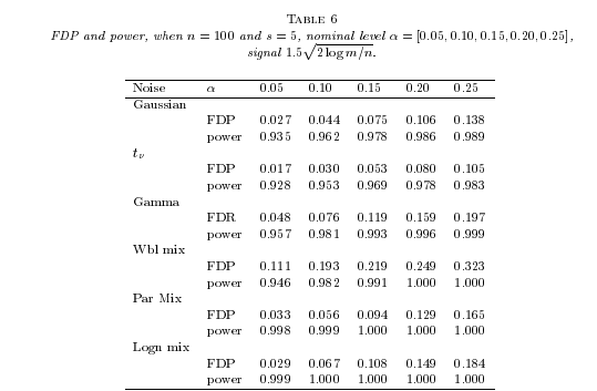 Figure 1
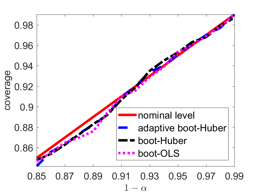 Figure 2
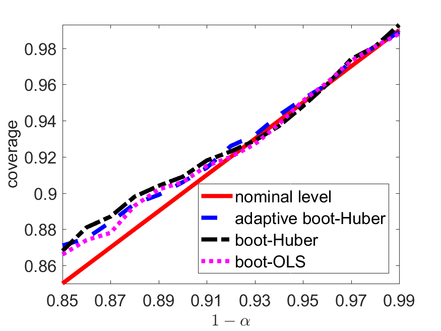 Figure 3
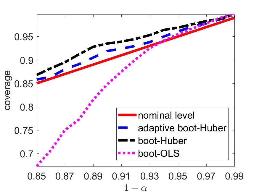 Figure 4
 Figure 5
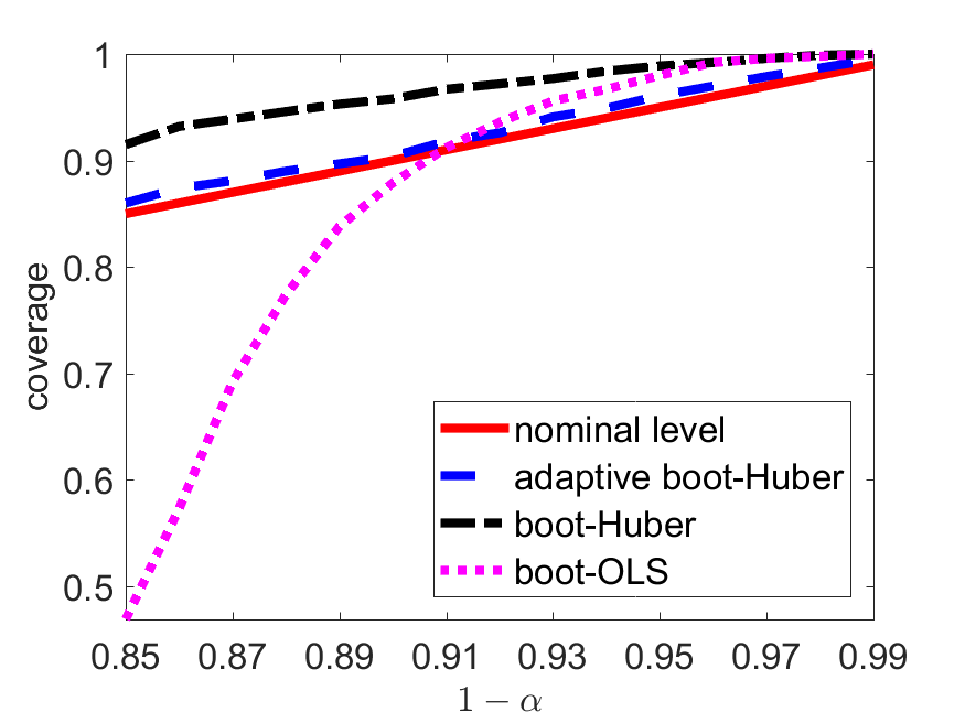 Figure 6
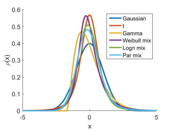 Figure 7
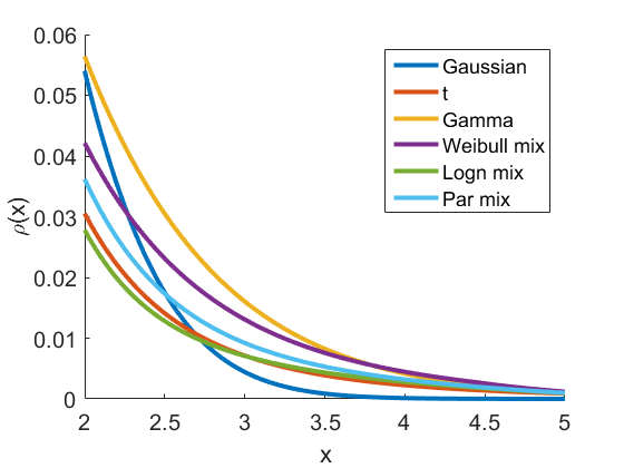 Figure 8
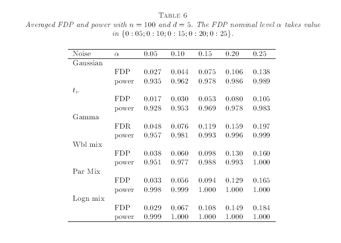 Figure 9
| Noise | Approach | |||||
| Gaussian | ||||||
| boot-Huber | 0.954 | 0.908 | 0.842 | 0.783 | 0.734 | |
| boot-OLS | 0.952 | 0.908 | 0.837 | 0.785 | 0.735 | |
| boot-Huber | 0.966 | 0.904 | 0.848 | 0.801 | 0.748 | |
| boot-OLS | 0.954 | 0.887 | 0.798 | 0.710 | 0.630 | |
| Gamma | ||||||
| boot-Huber | 0.962 | 0.918 | 0.860 | 0.798 | 0.747 | |
| boot-OLS | 0.955 | 0.910 | 0.843 | 0.775 | 0.700 | |
| Wbl mix | ||||||
| boot-Huber | 0.962 | 0.907 | 0.851 | 0.797 | 0.758 | |
| boot-OLS | 0.944 | 0.899 | 0.808 | 0.775 | 0.680 | |
| Par mix | ||||||
| boot-Huber | 0.955 | 0.907 | 0.856 | 0.802 | 0.761 | |
| boot-OLS | 0.948 | 0.900 | 0.843 | 0.785 | 0.738 | |
| Logn mix | ||||||
| boot-Huber | 0.958 | 0.912 | 0.860 | 0.782 | 0.744 | |
| boot-OLS | 0.954 | 0.912 | 0.796 | 0.682 | 0.616 | |
| Noise | Approach | |||||
| Gaussian | ||||||
| boot-Huber | 0.957 | 0.910 | 0.850 | 0.790 | 0.736 | |
| boot-OLS | 0.955 | 0.907 | 0.850 | 0.789 | 0.736 | |
| boot-Huber | 0.958 | 0.906 | 0.848 | 0.798 | 0.749 | |
| boot-OLS | 0.940 | 0.863 | 0.772 | 0.684 | 0.599 | |
| Gamma | ||||||
| boot-Huber | 0.948 | 0.899 | 0.845 | 0.780 | 0.726 | |
| boot-OLS | 0.944 | 0.889 | 0.822 | 0.751 | 0.685 | |
| Wbl mix | ||||||
| boot-Huber | 0.954 | 0.889 | 0.837 | 0.775 | 0.713 | |
| boot-OLS | 0.939 | 0.865 | 0.784 | 0.695 | 0.621 | |
| Par mix | ||||||
| boot-Huber | 0.945 | 0.898 | 0.847 | 0.789 | 0.738 | |
| boot-OLS | 0.941 | 0.886 | 0.820 | 0.757 | 0.700 | |
| Logn mix | ||||||
| boot-Huber | 0.958 | 0.916 | 0.864 | 0.812 | 0.748 | |
| boot-OLS | 0.938 | 0.886 | 0.812 | 0.718 | 0.590 | |
| Approach | |||||||
| boot-Huber | |||||||
| 50 | 0.951 | 0.904 | 0.848 | 0.789 | 0.725 | ||
| 2 | 100 | 0.959 | 0.914 | 0.866 | 0.827 | 0.771 | |
| 200 | 0.954 | 0.917 | 0.856 | 0.814 | 0.756 | ||
| 50 | 0.982 | 0.945 | 0.876 | 0.826 | 0.752 | ||
| 5 | 100 | 0.966 | 0.917 | 0.855 | 0.802 | 0.760 | |
| 200 | 0.950 | 0.894 | 0.835 | 0.777 | 0.721 | ||
| 50 | 0.990 | 0.972 | 0.955 | 0.915 | 0.881 | ||
| 10 | 100 | 0.980 | 0.949 | 0.897 | 0.850 | 0.799 | |
| 200 | 0.970 | 0.922 | 0.864 | 0.826 | 0.777 | ||
| boot-OLS | |||||||
| 50 | 0.942 | 0.887 | 0.827 | 0.758 | 0.672 | ||
| 2 | 100 | 0.956 | 0.901 | 0.849 | 0.785 | 0.714 | |
| 200 | 0.947 | 0.898 | 0.822 | 0.763 | 0.685 | ||
| 50 | 0.976 | 0.911 | 0.836 | 0.754 | 0.688 | ||
| 5 | 100 | 0.954 | 0.896 | 0.824 | 0.751 | 0.674 | |
| 200 | 0.940 | 0.868 | 0.790 | 0.698 | 0.622 | ||
| 50 | 0.997 | 0.970 | 0.919 | 0.844 | 0.761 | ||
| 10 | 100 | 0.975 | 0.921 | 0.850 | 0.784 | 0.719 | |
| 200 | 0.954 | 0.879 | 0.816 | 0.731 | 0.650 |
| Noise | Approach | 0.99 | 0.97 | 0.95 | 0.90 | 0.87 |
| adaptive boot-Huber | 0.993 | 0.970 | 0.942 | 0.896 | 0.868 | |
| boot-Huber | 0.991 | 0.971 | 0.946 | 0.899 | 0.868 | |
| boot-OLS | 0.993 | 0.970 | 0.948 | 0.895 | 0.868 | |
| adaptive boot-Huber | 0.994 | 0.978 | 0.961 | 0.919 | 0.880 | |
| boot-Huber | 0.997 | 0.983 | 0.969 | 0.935 | 0.895 | |
| boot-OLS | 0.997 | 0.978 | 0.955 | 0.848 | 0.750 | |
| adaptive boot-Huber | 0.994 | 0.980 | 0.961 | 0.916 | 0.882 | |
| boot-Huber | 1.000 | 0.992 | 0.978 | 0.948 | 0.921 | |
| boot-OLS | 0.999 | 0.989 | 0.972 | 0.864 | 0.710 | |
| adaptive boot-Huber | 0.995 | 0.979 | 0.961 | 0.904 | 0.881 | |
| boot-Huber | 1.000 | 0.996 | 0.989 | 0.958 | 0.939 | |
| boot-OLS | 1.000 | 0.996 | 0.980 | 0.879 | 0.692 |
| Noise | Approach | |||||
| Gaussian | ||||||
| boot-Huber | 0.210 | 0.301 | 0.365 | 0.412 | 0.443 | |
| boot-OLS | 0.214 | 0.299 | 0.365 | 0.416 | 0.446 | |
| boot-Huber | 0.191 | 0.295 | 0.364 | 0.399 | 0.442 | |
| boot-OLS | 0.222 | 0.336 | 0.420 | 0.467 | 0.491 | |
| Gamma | ||||||
| boot-Huber | 0.191 | 0.292 | 0.366 | 0.410 | 0.441 | |
| boot-OLS | 0.220 | 0.309 | 0.384 | 0.423 | 0.456 | |
| Wbl mix | ||||||
| boot-Huber | 0.176 | 0.265 | 0.343 | 0.392 | 0.435 | |
| boot-OLS | 0.201 | 0.308 | 0.392 | 0.440 | 0.472 | |
| Par mix | ||||||
| boot-Huber | 0.181 | 0.286 | 0.358 | 0.408 | 0.443 | |
| boot-OLS | 0.196 | 0.324 | 0.414 | 0.466 | 0.488 | |
| Logn mix | ||||||
| boot-Huber | 0.176 | 0.268 | 0.331 | 0.392 | 0.425 | |
| boot-OLS | 0.189 | 0.327 | 0.416 | 0.461 | 0.488 | |
| Noise | Approach | |||||
| Gaussian | ||||||
| boot-Huber | 0.232 | 0.333 | 0.390 | 0.427 | 0.456 | |
| boot-OLS | 0.236 | 0.340 | 0.388 | 0.431 | 0.455 | |
| boot-Huber | 0.205 | 0.291 | 0.357 | 0.407 | 0.445 | |
| boot-OLS | 0.236 | 0.342 | 0.437 | 0.481 | 0.497 | |
| Gamma | ||||||
| boot-Huber | 0.212 | 0.295 | 0.358 | 0.401 | 0.440 | |
| boot-OLS | 0.232 | 0.307 | 0.366 | 0.415 | 0.451 | |
| Wbl mix | ||||||
| boot-Huber | 0.194 | 0.292 | 0.364 | 0.409 | 0.439 | |
| boot-OLS | 0.220 | 0.335 | 0.409 | 0.447 | 0.480 | |
| Par mix | ||||||
| boot-Huber | 0.168 | 0.252 | 0.333 | 0.395 | 0.433 | |
| boot-OLS | 0.189 | 0.314 | 0.415 | 0.469 | 0.495 | |
| Logn mix | ||||||
| boot-Huber | 0.232 | 0.314 | 0.379 | 0.418 | 0.447 | |
| boot-OLS | 0.245 | 0.363 | 0.452 | 0.491 | 0.500 | |
| Noise | Approach | |||||
| Gaussian | ||||||
| boot-Huber | 0.946 | 0.898 | 0.848 | 0.781 | 0.725 | |
| boot-OLS | 0.944 | 0.898 | 0.843 | 0.782 | 0.720 | |
| boot-Huber | 0.968 | 0.919 | 0.877 | 0.825 | 0.777 | |
| boot-OLS | 0.954 | 0.881 | 0.803 | 0.729 | 0.642 | |
| Gamma | ||||||
| boot-Huber | 0.961 | 0.911 | 0.868 | 0.812 | 0.751 | |
| boot-OLS | 0.958 | 0.900 | 0.842 | 0.778 | 0.716 | |
| Wbl mix | ||||||
| boot-Huber | 0.963 | 0.907 | 0.866 | 0.808 | 0.748 | |
| boot-OLS | 0.947 | 0.880 | 0.817 | 0.724 | 0.663 | |
| Par mix | ||||||
| boot-Huber | 0.974 | 0.928 | 0.882 | 0.842 | 0.775 | |
| boot-OLS | 0.963 | 0.897 | 0.815 | 0.715 | 0.634 | |
| Logn mix | ||||||
| boot-Huber | 0.972 | 0.936 | 0.888 | 0.834 | 0.780 | |
| boot-OLS | 0.962 | 0.901 | 0.804 | 0.701 | 0.615 | |
| Noise | Approach | |||||
| Gaussian | ||||||
| boot-Huber | 0.953 | 0.893 | 0.844 | 0.799 | 0.743 | |
| boot-OLS | 0.955 | 0.893 | 0.846 | 0.798 | 0.744 | |
| boot-Huber | 0.960 | 0.910 | 0.850 | 0.795 | 0.750 | |
| boot-OLS | 0.948 | 0.860 | 0.759 | 0.657 | 0.586 | |
| Gamma | ||||||
| boot-Huber | 0.949 | 0.896 | 0.836 | 0.782 | 0.729 | |
| boot-OLS | 0.947 | 0.886 | 0.817 | 0.765 | 0.704 | |
| Wbl mix | ||||||
| boot-Huber | 0.957 | 0.906 | 0.861 | 0.811 | 0.766 | |
| boot-OLS | 0.941 | 0.879 | 0.805 | 0.722 | 0.656 | |
| Par mix | ||||||
| boot-Huber | 0.963 | 0.924 | 0.862 | 0.798 | 0.743 | |
| boot-OLS | 0.958 | 0.869 | 0.751 | 0.669 | 0.581 | |
| Logn mix | ||||||
| boot-Huber | 0.958 | 0.909 | 0.849 | 0.795 | 0.739 | |
| boot-OLS | 0.947 | 0.861 | 0.723 | 0.600 | 0.531 | |
| Noise | Approach | |||||
| Gaussian | ||||||
| boot-Huber | 0.954 | 0.899 | 0.842 | 0.783 | 0.732 | |
| boot-OLS | 0.952 | 0.901 | 0.842 | 0.778 | 0.726 | |
| boot-Huber | 0.962 | 0.904 | 0.843 | 0.802 | 0.734 | |
| boot-OLS | 0.948 | 0.870 | 0.772 | 0.678 | 0.594 | |
| Gamma | ||||||
| boot-Huber | 0.962 | 0.906 | 0.841 | 0.786 | 0.736 | |
| boot-OLS | 0.949 | 0.893 | 0.820 | 0.767 | 0.706 | |
| Wbl mix | ||||||
| boot-Huber | 0.968 | 0.924 | 0.864 | 0.811 | 0.747 | |
| boot-OLS | 0.958 | 0.894 | 0.811 | 0.737 | 0.665 | |
| Par mix | ||||||
| boot-Huber | 0.966 | 0.910 | 0.849 | 0.790 | 0.733 | |
| boot-OLS | 0.960 | 0.881 | 0.780 | 0.681 | 0.609 | |
| Logn mix | ||||||
| boot-Huber | 0.968 | 0.922 | 0.875 | 0.811 | 0.763 | |
| boot-OLS | 0.963 | 0.878 | 0.778 | 0.693 | 0.608 | |
| Noise | Approach | |||||
| Gaussian | ||||||
| boot-Huber | 0.943 | 0.873 | 0.813 | 0.761 | 0.706 | |
| boot-OLS | 0.941 | 0.867 | 0.815 | 0.754 | 0.708 | |
| boot-Huber | 0.956 | 0.907 | 0.850 | 0.791 | 0.729 | |
| boot-OLS | 0.941 | 0.865 | 0.744 | 0.639 | 0.561 | |
| Gamma | ||||||
| boot-Huber | 0.953 | 0.904 | 0.849 | 0.799 | 0.738 | |
| boot-OLS | 0.943 | 0.895 | 0.841 | 0.779 | 0.717 | |
| Wbl mix | ||||||
| boot-Huber | 0.961 | 0.906 | 0.843 | 0.788 | 0.739 | |
| boot-OLS | 0.949 | 0.871 | 0.788 | 0.724 | 0.641 | |
| Par mix | ||||||
| boot-Huber | 0.971 | 0.932 | 0.873 | 0.807 | 0.751 | |
| boot-OLS | 0.963 | 0.889 | 0.779 | 0.674 | 0.572 | |
| Logn mix | ||||||
| boot-Huber | 0.943 | 0.889 | 0.826 | 0.775 | 0.725 | |
| boot-OLS | 0.936 | 0.844 | 0.715 | 0.597 | 0.516 | |
| Noise | 0.05 | 0.10 | 0.15 | 0.20 | 0.25 | |
| Gaussian | ||||||
| FDP | 0.027 | 0.044 | 0.075 | 0.106 | 0.138 | |
| Power | 0.935 | 0.962 | 0.978 | 0.986 | 0.989 | |
| FDP | 0.017 | 0.030 | 0.053 | 0.080 | 0.105 | |
| Power | 0.928 | 0.953 | 0.969 | 0.978 | 0.983 | |
| Gamma | ||||||
| FDP | 0.048 | 0.076 | 0.119 | 0.159 | 0.197 | |
| Power | 0.957 | 0.981 | 0.993 | 0.996 | 0.999 | |
| Wbl mix | ||||||
| FDP | 0.038 | 0.060 | 0.098 | 0.130 | 0.160 | |
| Power | 0.951 | 0.977 | 0.988 | 0.993 | 1.000 | |
| Par mix | ||||||
| FDP | 0.033 | 0.056 | 0.094 | 0.129 | 0.165 | |
| Power | 0.998 | 0.999 | 1.000 | 1.000 | 1.000 | |
| Logn mix | ||||||
| FDP | 0.029 | 0.067 | 0.108 | 0.149 | 0.184 | |
| Power | 0.999 | 1.000 | 1.000 | 1.000 | 1.000 |
| 0.05 | 0.10 | 0.15 | 0.20 | 0.25 | |||
| 2 | 100 | FDP | 0.061 | 0.098 | 0.143 | 0.186 | 0.232 |
| Power | 0.981 | 0.991 | 0.995 | 0.997 | 0.998 | ||
| 200 | FDP | 0.048 | 0.101 | 0.149 | 0.195 | 0.242 | |
| Power | 0.989 | 0.995 | 0.997 | 0.998 | 0.998 | ||
| 5 | 100 | FDP | 0.038 | 0.060 | 0.098 | 0.130 | 0.160 |
| Power | 0.951 | 0.977 | 0.988 | 0.993 | 1.000 | ||
| 200 | FDP | 0.056 | 0.092 | 0.137 | 0.180 | 0.223 | |
| Power | 0.938 | 0.991 | 0.996 | 0.997 | 0.999 | ||
| 10 | 100 | FDP | 0.006 | 0.014 | 0.022 | 0.035 | 0.052 |
| Power | 0.607 | 0.825 | 0.897 | 0.940 | 0.961 | ||
| 200 | FDP | 0.043 | 0.070 | 0.110 | 0.145 | 0.187 | |
| Power | 0.971 | 0.983 | 0.989 | 0.993 | 0.995 |
| Noise | 0.05 | 0.10 | 0.15 | 0.20 | 0.25 | |
| Gaussian | ||||||
| FDP | 0.015 | 0.039 | 0.063 | 0.093 | 0.124 | |
| Power | 1.000 | 1.000 | 1.000 | 1.000 | 1.000 | |
| FDP | 0.009 | 0.027 | 0.046 | 0.072 | 0.098 | |
| Power | 0.999 | 1.000 | 1.000 | 1.000 | 1.000 | |
| Gamma | ||||||
| FDP | 0.038 | 0.063 | 0.103 | 0.136 | 0.178 | |
| Power | 1.000 | 1.000 | 1.000 | 1.000 | 1.000 | |
| Wbl mix | ||||||
| FDP | 0.038 | 0.049 | 0.089 | 0.120 | 0.156 | |
| Power | 0.999 | 1.000 | 1.000 | 1.000 | 1.000 | |
| Par mix | ||||||
| FDP | 0.037 | 0.060 | 0.100 | 0.135 | 0.167 | |
| Power | 1.000 | 1.000 | 1.000 | 1.000 | 1.000 | |
| Logn mix | ||||||
| FDP | 0.024 | 0.067 | 0.099 | 0.128 | 0.157 | |
| Power | 1.000 | 1.000 | 1.000 | 1.000 | 1.000 |
| 0.05 | 0.10 | 0.15 | 0.20 | 0.25 | |||
| 2 | 100 | FDP | 0.042 | 0.087 | 0.125 | 0.179 | 0.221 |
| Power | 1.000 | 1.000 | 1.000 | 1.000 | 1.000 | ||
| 200 | FDP | 0.049 | 0.102 | 0.144 | 0.187 | 0.234 | |
| Power | 1.000 | 1.000 | 1.000 | 1.000 | 1.000 | ||
| 5 | 100 | FDP | 0.026 | 0.049 | 0.089 | 0.120 | 0.156 |
| Power | 0.999 | 1.000 | 1.000 | 1.000 | 1.000 | ||
| 200 | FDP | 0.040 | 0.069 | 0.089 | 0.132 | 0.184 | |
| Power | 1.000 | 1.000 | 1.000 | 1.000 | 1.000 | ||
| 10 | 100 | FDP | 0.011 | 0.014 | 0.022 | 0.041 | 0.054 |
| Power | 0.991 | 0.995 | 0.999 | 0.999 | 0.999 | ||
| 200 | FDP | 0.040 | 0.069 | 0.102 | 0.131 | 0.166 | |
| Power | 1.000 | 1.000 | 1.000 | 1.000 | 1.000 |
Peer Reviews
No public reviews on file for this paper yet. If you reviewed it on a platform where reviews are public (OpenReview, ICLR, NeurIPS, ICML), you can paste yours below so the community can read it here.
Videos
No videos yet. Explain this paper in a talk, walkthrough, or lecture? Add one.
Taxonomy
TopicsStatistical Methods and Inference · Advanced Statistical Methods and Models · Statistical Methods and Bayesian Inference
Robust Inference via Multiplier Bootstrap
Xi Chen and Wen-Xin Zhou Stern School of Business, New York University, New York, NY 10012, USA. E-mail: [email protected].Department of Mathematics, University of California, San Diego, La Jolla, CA 92093, USA. E-mail: [email protected]. Supported in part by NSF Grant DMS-1811376.
Abstract
This paper investigates the theoretical underpinnings of two fundamental statistical inference problems, the construction of confidence sets and large-scale simultaneous hypothesis testing, in the presence of heavy-tailed data. With heavy-tailed observation noise, finite sample properties of the least squares-based methods, typified by the sample mean, are suboptimal both theoretically and empirically. In this paper, we demonstrate that the adaptive Huber regression, integrated with the multiplier bootstrap procedure, provides a useful robust alternative to the method of least squares. Our theoretical and empirical results reveal the effectiveness of the proposed method, and highlight the importance of having inference methods that are robust to heavy tailedness.
Keywords: Confidence set; heavy-tailed data; multiple testing; multiplier bootstrap; robust regression; Wilks’ theorem.
1 Introduction
In classical statistical analysis, it is typically assumed that data are drawn from a Gaussian distribution. Although the normality assumption has been widely adopted to facilitate methodological development and theoretical analysis, Gaussian models could be an idealization of the complex random world. The non-Gaussian, or even heavy-tailed, character of the distribution of empirical data has been repeatedly observed in various domains, ranging from genomics, medical imaging to economics and finance. New challenges are thus brought to classical statistical methods. For linear models, regression estimators based on the least squares loss are suboptimal, both theoretically and empirically, in the presence of heavy-tailed errors. The necessity of robust alternatives to least squares was first noticed by Peter Huber in his seminal work “Robust Estimation of a Location Parameter” (Huber, 1964). Due to the growing complexity of modern data, the notion of robustness is becoming increasingly important in statistical analysis and finds its use in a wide range of applications. We refer to Huber and Ronchetti (2009) for an overview of robust statistics.
Although the past a few decades have witnessed the active development of rich statistical theory on robust estimation, robust statistical inference for heavy-tailed data has always been a challenging problem on which the extant literature has been somewhat silent. Fan, Hall and Yao (2007), Delaigle, Hall and Jin (2011) and Liu and Shao (2014) investigated robust inference that is confined to the Student’s -statistic. However, as pointed out by Devroye et al. (2016) (see Section 8 therein), sharp confidence estimation for heavy-tailed data in the finite sample set-up remains an open problem and a general methodology is still lacking. To that end, this paper makes a further step in studying confidence estimation from a robust perspective. In particular, under linear model with heavy-tailed errors, we address two fundamental problems: (1) confidence set construction for regression coefficients, and (2) large-scale multiple testing with the guarantee of false discovery rate control. The developed techniques provide mathematical underpinnings for a class of robust statistical inference problems. Moreover, sharp exponential-type bounds for the coverage probability of the confidence set are derived under weak moment assumptions.
1.1 Confidence sets
Consider the linear model , where denotes the response variable, is the (random) vector of covariates, is the vector of regression coefficients and represents the regression error satisfying and . Assume that we observe a random sample from :
[TABLE]
The intercept term is implicitly assumed in model (1.1) by taking the first element of to be one so that the first element of becomes the intercept. The least squares estimator and its variations have been widely adopted to estimate , which on many occasions achieve the minimax rate in terms of the mean squared error (MSE).
Although the MSE plays an important role in estimation, an estimator that is optimal in MSE might be suboptimal in terms of non-asymptotic deviation, which often relates to the construction of confidence intervals. For example, in the mean estimation problem, although the sample mean has an optimal minimax mean squared error among all mean estimators, its deviation is worse for non-Gaussian samples than for Gaussian ones, and the worst-case deviation is suboptimal when the sampling distribution has heavy tails (Catoni, 2012). More specifically, let be independent random variables from with mean and variance . Consider the empirical mean , applying Chebyshev’s inequality delivers a polynomial-type deviation bound
[TABLE]
In addition, if the distribution of is sub-Gaussian, i.e. for all , then following the terminology in Devroye et al. (2016), becomes a sub-Gaussian estimator in the sense that
[TABLE]
Catoni (2012) established a lower bound for the deviations of when the sampling distribution is the least favorable in the class of all distributions with bounded variance: for any , there is some distribution with mean and variance such that an independent sample of size drawn from it satisfies
[TABLE]
This shows that the deviation bound obtained from Chebyshev’s inequality is essentially sharp under finite variance condition. The limitation of least squares method arises also in the regression setting, which triggers an outpouring of interest in developing sub-Gaussian estimators, from univariate mean estimation to multivariate or even high dimensional problems, for heavy-tailed data to achieve sharp deviation bounds from a non-asymptotic viewpoint. See, for example, Brownlees, Joly and Lugosi (2015), Minsker (2015, 2018), Hsu and Sabato (2016), Devroye et al. (2016), Catoni and Giulini (2017), Giulini (2017), Fan, Li and Wang (2017), Sun et al. (2018) and Lugosi and Mendelson (2019), among others. In particular, Fan, Li and Wang (2017) and Sun et al. (2018) proposed adaptive (regularized) Huber estimators with diverging robustification parameters (see Definition 2.1 in Section 2.1), and derived exponential-type deviation bounds when the error distribution only has finite variance. Their key observation is that the robustification parameter should adapt to the sample size, dimensionality and noise level for optimal tradeoff between bias and robustness.
All the aforementioned work studies robust estimation through concentration properties, that is, the robust estimator is tightly concentrated around the true parameter with high probability even when the sampling distribution has only a small number of finite moments. In general, concentration inequalities loose constant factors and may result in confidence intervals too wide to be informative. Therefore, an interesting and challenging open problem is how to construct tight confidence sets for with finite samples of heavy-tailed data (Devroye et al., 2016).
This paper addresses this open problem by developing a robust inference framework with non-asymptotic guarantees. To illustrate the key idea, we focus on the classical setting where the parameter dimension is smaller than but is allowed to increase with the number of observations . Our approach integrates concentration properties of the adaptive Huber estimator (see Theorems 2.1 and 2.2) and the multiplier bootstrap method. The multiplier bootstrap, also known as the weighted bootstrap, is one of the most widely used resampling methods for constructing a confidence interval/set or for measuring the significance of a test. Its theoretical validity is typically guaranteed by the multiplier central limit theorem (van der Vaart and Wellner, 1996). We refer to Chatterjee and Bose (2005), Arlot, Blanchard and Roquain (2010), Chernozhukov, Chetverikov and Kato (2013, 2014), Spokoiny and Zhilova (2015) and Zhilova (2016) for the most recent progress in the theory and applications of the multiplier bootstrap. In particular, Spokoiny and Zhilova (2015) considered a multiplier bootstrap procedure for constructing likelihood-based confidence sets under a possible model misspecification. For a linear model with sub-Gaussian errors, their results validate the bootstrap procedure when applied to the ordinary least squares (OLS). With heavy-tailed errors in the regression model (1.1), we demonstrate how the adaptive Huber regression and the multiplier bootstrap can be integrated to construct robust and sharp confidence sets for the true parameter with a given coverage probability. The validity of the bootstrap procedure in situations with a limited sample size, growing dimensionality and heavy-tailed errors is established. In all these theoretical results, we provide non-asymptotic bounds for the errors of bootstrap approximation. See Theorems 2.3 and 2.4 for finite sample properties of the bootstrap adaptive Huber estimator, including the deviation inequality, Bahadur representation and Wilks’ expansion.
An alternative robust inference method is based on the asymptotic theory developed in Zhou et al. (2018); see, for example, Theorems 2.2 and 2.3 therein. Since the asymptotic distribution of either the proposed robust estimator itself or the excess risk depends on , a direct approach is to replace by some sub-Gaussian variance estimator using Catoni’s method (Catoni, 2012) or the median-of-means technique (Minsker, 2015), with the advantage of being computationally fast. The disadvantage, however, is two-fold: first, constructing sub-Gaussian variance estimator involves another tuning parameter (for the problem of simultaneously testing regression models as discussed in the next section, variance estimation brings additional tuning parameters); secondly, because the squared heavy-tailed data is highly right-skewed, using the method in Catoni (2012) or Fan, Li and Wang (2017) tends to underestimate the variance, and the median-of-means method is numerically unstable for small or moderate samples. Both two methods were examined numerically in Zhou et al. (2018), while the multiplier bootstrap procedure, albeit being more computationally intensive, demonstrates the most desirable finite sample performance.
1.2 Simultaneous inference
In addition to building confidence sets for an individual parameter vector, multiple hypothesis testing is another important statistical problem with applications to many scientific fields, where thousands of tests are performed simultaneously (Dudoit and van der Laan, 2008; Efron, 2010). Gene microarrays comprise a prototypical example; there, each subject is automatically measured on tens of thousands of features. Together, the large number of tests together with heavy tailedness bring new challenges to conventional statistical methods, which, in this scenario, often suffer from low power to detect important features and poor reproducibility. Robust alternatives are thus needed for conducting large-scale multiple inference for heavy-tailed data.
In this section, we consider the multiple response regression model
[TABLE]
where is the intercept, are -dimensional vectors of random covariates and regression coefficients, respectively, and is the regression error. Since our main focus here is the inference for intercepts, we decompose the parameter vector in (1.1) into two parts: the intercept and the slope . Moreover, we use in (1.2) to distinguish from in (1.1). Write and let be the vector of intercepts. Based on random samples from model (1.2), our goal is to simultaneously test the hypotheses
[TABLE]
An iconic example of model (1.2) is the linear pricing model, which subsumes the capital asset pricing model (CAPM) (Sharpe, 1964; Lintner, 1965) and the Fama-French three-factor model (Fama and French, 1993). The key implication from the multi-factor pricing theory is that for any asset , the intercept should be zero. It is then important to investigate if such a pricing theory, also known as the “mean-variance efficiency” pricing, can be validated by empirical data (Fan, Liao and Yao, 2015). According to the Berk and Green equilibrium (Berk and Green, 2004), inefficient pricing by the market may occur to a small proportion of exceptional assets, namely a very small fraction of the ’s are nonzero. To identify positive ’s by testing a large number of hypotheses simultaneously, Barras, Scaillet and Wermers (2010) and Lan and Du (2019) developed FDR controlling procedures for data coming from model (1.2), which can be applied to mutual fund selection in empirical finance. We refer to Friguet, Kloareg and Causeur (2009), Desai and Storey (2012), Fan, Han and Gu (2012) and Wang et al. (2017) for more examples from gene expression studies, where the goal is to identify features showing a biological signal of interest.
Despite the extensive research and wide application of this problem, existing least squares-based methods with normal calibration could fail when applied to heavy-tailed data with a small sample size. To address this challenge, we develop a robust bootstrap procedure for large-scale simultaneous inference, which achieves good numerical performance for a small or moderate sample size. Theoretically, we prove its validity on controlling the false discover proportion (FDP) (see Theorem 4.1).
Finally, we briefly comment on the computation issue. Fast computation of Huber regression is critical to our procedure since the multiplier bootstrap requires solving Huber loss minimization for at least hundreds of times. Ideally, a second order approach (e.g. Newton’s method) is preferred. However, the second order derivative of Huber loss does not exist everywhere. To address this issue, we adopt the damped semismooth Netwon method (Qi and Sun, 1999), which is a synergic integration of first and second order methods. The details are provided in Appendix D of the supplemental material.
1.3 Organization of the paper
The rest of the paper proceeds as follows. Section 2.1 presents a series of finite sample results of the adaptive Huber regression. Sections 2.2 and 2.3 contain, respectively, the description of the bootstrap procedure for building confidence sets and theoretical guarantees. Two data-driven schemes are proposed in Section 3 for choosing the tuning parameter in the Huber loss. In Section 4, we propose a robust bootstrap calibration method for multiple testing and investigate its theoretical property on controlling the FDP. The conclusions that are drawn in Sections 2 and 4 are illustrated numerically in Section 5. We conclude with a discussion in Section 6. The supplementary material contains all the proofs and additional simulation studies.
1.4 Notation
Let us summarize our notation. For every integer , we use to denote the the -dimensional Euclidean space. The inner product of any two vectors is defined by . We use the notation for the -norms of vectors in : and . For , denotes the unit sphere in . Throughout this paper, we use bold capital letters to represent matrices. For , represents the identity/unit matrix of size . For any symmetric matrix , is the operator norm of . We use and to denote the largest and smallest eigenvalues of , respectively. For any two real numbers and , we write and . For two sequences of non-negative numbers and , indicates that there exists a constant independent of such that ; is equivalent to ; is equivalent to and . For two numbers and , we write if depends only on . For any set , we use and to denote its cardinality, i.e. the number of elements in .
2 Robust bootstrap confidence sets
2.1 Preliminaries
First, we present some finite sample properties of the adaptive Huber estimator, which are of independent interest and also sharpen the results in Sun et al. (2018).
Let us recall the definition of Huber loss,
Definition 2.1**.**
The Huber loss (Huber, 1964) is defined as
[TABLE]
where is a tuning parameter and will be referred to as the robustification parameter that balances bias and robustness.
The Huber estimator is defined as
[TABLE]
The following theorem provides a sub-Gaussian-type deviation inequality and a non-asymptotic Bahadur representation for . The proof is given in the supplement. We first impose the moment conditions.
Assumption 1**.**
(i) There exists some constant such that for any and , , where and is positive definite. (ii) The regression error satisfies , and almost surely for some .
Part (i) of Condition 1 requires to be a sub-Gaussian vector. Via one-dimensional marginal, this generalizes the concept of sub-Gaussian random variables to higher dimensions. Typical examples include: (i) Gaussian and Bernoulli random vectors, (ii) spherical random vector111A random vector is said to have a spherical distribution if it is uniformly distributed on the Euclidean sphere in with center at the origin and radius . , (iii) random vector that is uniformly distributed on the Euclidean ball centered at the origin with radius , and (iv) random vector that is uniformly distributed on the unit cube . In all the above cases, the constant represents a dimension-free constant. We refer to Chapter 3.4 in Vershynin (2018) for detailed discussions of sub-Gaussian distributions in higher dimensions. Technically, this assumption is needed in order to derive an exponential-type concentration inequality for the quadratic form , where
[TABLE]
Theorem 2.1**.**
Assume Condition 1 holds. For any and , the estimator given in (2.4) with satisfies
[TABLE]
as long as , where – are constants depending only on .
The non-asymptotic results in Theorem 2.1 reveal a new perspective for Huber’s method: to construct sub-Gaussian estimators for linear regression with heavy-tailed errors, the tuning parameter in the Huber loss should adapt to the sample size, dimension and moments for optimal tradeoff between bias and robustness. The resulting estimator is therefore referred to as the adaptive Huber estimator. Specifically, Theorem 2.1 provides the concentration property of the adaptive Huber estimator and the Fisher expansion for the difference . It improves Theorem 2.1 in Zhou et al. (2018) by sharpening the sample size scaling. The classical asymptotic results can be easily derived from the obtained non-asymptotic expansions. In the following theorem, we further study the concentration property of the Wilks’ expansion for the excess . This new result is directly related to the construction of confidence sets. See Theorem 2.3 below for its counterpart in the bootstrap world.
Theorem 2.2**.**
Assume Condition 1 holds. Then for any and , the estimator with satisfies that with probability at least ,
[TABLE]
as long as , where are constants depending on .
Remark 1** (On the robustification parameter ).**
Going through the proofs of Theorems 2.1 and 2.2, we see that the robustification parameter can be chosen as
[TABLE]
such that the conclusions (2.6)–(2.9) hold as long as . This implies that the existence of higher moments of increases the flexibility of choosing , whose order ranges from to . In practice, is unknown and thus brings difficulty in calibrating . Guided by the theoretical results, in Section 3 we propose a data-dependent procedure to choose .
Remark 2** (Sample size scaling).**
The deviation inequalities in Theorems 2.1 and 2.2 hold under the scaling condition , indicating that as many as samples are required to guarantee the finite sample properties of the estimator. Similar conditions are also imposed for Proposition 2.4 in Catoni (2012) and Theorem 3.1 in Audibert and Catoni (2011). In particular if , taking and , the corresponding estimator satisfies
[TABLE]
with probability at least under the scaling . From an asymptotic viewpoint, this implies that if the dimension , as a function of , satisfies as , then for any deterministic vector , the distribution of the linear contrast coincides with that of asymptotically.
Remark 3**.**
To achieve sub-Gaussian behavior, the choice of loss function is not unique. An alternative loss function, which is obtained from the influence function proposed by Catoni and Giulini (2017), is
[TABLE]
The function is convex, twice differentiable everywhere and has bounded derivative that for all . By modifying the proofs of Theorems 2.1 and 2.2, it can be shown that the theoretical properties of the adaptive Huber estimator remain valid for the estimator that minimizes the empirical -loss. Computationally, it can be solved via Newton’s method.
2.2 Multiplier bootstrap
In this section, we go beyond estimation and focus on robust inference. According to (2.9), the distribution of is close to that of provided that is small, where . As we will see in the proof of Theorem 2.5 that, the truncated random variable has mean and variance approximately equal to [math] and , respectively. Heuristically, the multivariate central limit theorem allows us to approximate the distribution of the normalized sum by . If this were true, then the distribution of is close to the scaled chi-squared distribution with degrees of freedom. This is in line with the asymptotic behavior of the likelihood ratio statistic that was studied in Wilks (1938). With sample size sufficiently large, this result allows to construct confidence sets for using quantiles of : for any ,
[TABLE]
where denotes the upper -quantile of . Estimating the residual variance in the construction of is even more challenging when the errors are heavy-tailed. Moreover, as argued in Spokoiny and Zhilova (2015), a possibly low speed of convergence of the likelihood ratio statistic makes the asymptotic Wilks’ result hardly applicable to the case of small or moderate samples. Motivated by these two concerns, we have the following goal:
[TABLE]
The results in Section 2.1 show that the adaptive Huber estimator provides a robust estimate of in the sense that it admits sub-Gaussian-type deviations when the error distribution only has finite variance. To estimate the quantiles of the adaptive Huber estimator and to construct confidence set, we consider the use of multiplier bootstrap. Let be independent and identically distributed (IID) random variables that are independent of the observed data and satisfy
[TABLE]
With denoting the random weights, the bootstrap Huber loss and bootstrap Huber estimator are defined, respectively, as
[TABLE]
where is a prespecified radius parameter. A simple observation is that , where is the conditional expectation given the observed data . Therefore, and the difference mimics .
Based on this idea, we propose a Huber regression based inference procedure in Algorithm 1, where the bootstrap threshold approximates
[TABLE]
Here is the probability measure with respect to the underlying data generating process.
2.3 Theoretical results
In this section, we present detailed theoretical results for the bootstrap adaptive Huber estimator, including the deviation inequality, non-asymptotic Bahadur representation (Theorem 2.3), and Wilks’ expansions (Theorem 2.4). Moreover, Theorems 2.5 and 2.6 establish the validity of the multiplier bootstrap for estimating quantiles of when the variance is unknown. Proofs of the finite sample properties of the bootstrap estimator require new techniques and are more involved than those of Theorems 2.1 and 2.2. We leave them to the supplemental material.
Assumption 2**.**
are IID from a random variable satisfying , and for all .
Theorem 2.3**.**
Assume Condition 1 with and Condition 2 hold. For any and , the estimator with and satisfies:
with probability (over ) at least ,
[TABLE] 2. 2.
with probability (over ) at least ,
[TABLE]
as long as , where – are positive constants depending on , and is the condition number of .
The following theorem is a bootstrap version of Theorem 2.2. Define the random process
[TABLE]
From (2.5) and (2.15) we see that
[TABLE]
In particular, write .
Theorem 2.4**.**
Assume Condition 1 with and Condition 2 hold. For any and , the bootstrap estimator with and satisfies that, with probability (over ) at least ,
[TABLE]
and
[TABLE]
as long as , where are constants depending only on .
The results (2.21) and (2.22) are non-asymptotic bootstrap versions of the Wilks’ and square-root Wilks’ phenomena. In particular, the latter indicates that the square-root excess is close to with high probability as long as the dimension of the parameter space satisfies the condition that is small.
Remark 4** (Order of robustification parameter).**
Similar to Remark 2.10, now with finite fourth moment , the robustification parameter in Theorems 2.3 and 2.4 can be chosen as
[TABLE]
such that the same conclusions remain valid. Due to Lemma A.2 in the supplemental material, here we require to be strictly less than .
The next result validates the approximation of the distribution of by that of in the Kolmogorov distance. Recall that denotes the conditional probability given the observed data .
Theorem 2.5**.**
Suppose Assumption 1 holds with and Condition 2 holds with . For any and , let for some . Then, with probability (over ) at least , it holds for any that
[TABLE]
where
[TABLE]
with .
Theorem 2.5 is in parallel with and can be viewed as a partial extension of Theorem 2.1 in Spokoiny and Zhilova (2015) to the case of heavy-tailed errors. In particular, taking in Theorem 2.5 we see that the error term scales as , while in Spokoiny and Zhilova (2015) it is of order . The difference is due to the fact that the latter allows misspecified models as discussed in Remark A.2 therein. In some way, allowing asymmetric and heavy-tailed errors can be regarded as a particular form of misspecification, considering that the OLS is the maximum likelihood estimator at the normal model.
Remark 5** (Asymptotic result).**
To make asymptotic statements, we assume with an understanding that depends on and possibly as . Theorem 2.5 can be used to show the bootstrap consistency, where the notion of consistency is the one that guarantees asymptotically valid inference. Specifically, it shows that when the dimension , as a function of , satisfies , then with for some , it holds
[TABLE]
as .
For any , let
[TABLE]
be the upper -quantile of under , which serves as an approximate to the target value given in (2.17). As a direct consequence of Theorem 2.5, the following result formally establishes the validity of the multiplier bootstrap for adaptive Huber regression with heavy-tailed error.
Theorem 2.6** (Validity of multiplier bootstrap).**
Assume the conditions of Theorem 2.5 hold and take . Then, for any ,
[TABLE]
where , where . In particular, taking , it holds
[TABLE]
provided that satisfies as .
3 Data-driven procedures for choosing
The theoretical results in Sections 2.1 and 2.3 reveal that how the Huber-type estimator would perform under various idealized scenarios, as such providing guidance on the choice of the key tuning parameter, which is referred to as the robustification parameter that balances bias and robustness. For estimation purpose, we take with ; and for bootstrap inference, we choose with . Since both and are typically unknown in practice, an intuitive approach is replace them by the empirical second and fourth moments of the residuals from the ordinary least squares (OLS) estimator, i.e. and . This simple approach performs reasonably well empirically (see Section 5). However, when heavy tails may be a concern, and are not good estimates of and . In this section, we discuss two data-dependent methods for choosing the tuning parameter : the first one uses an adaptive technique based on Lepski’s method (Lepskiĭ, 1991), and the second method is inspired by the censored equation approach in Hahn, Kuelbs and Weiner (1990) which was originally introduced in pursing a more robust weak convergence theory for self-normalized sums.
3.1 Lepski-type method
Borrowing an idea from Minsker (2018), we first consider a simple adaptive procedure based on Lepski’s method. Let and be some crude preliminary lower and upper bounds for the residual standard deviation, that is, . For some prespecified , let for and define
[TABLE]
It is easy to see that the set has its cardinality bounded by . Accordingly, we define a sequence of candidate parameters and let be the Huber estimator with . Set
[TABLE]
for some constant . The resulting adaptive estimator is then defined as .
Theorem 3.1**.**
Assume that for as in Theorem 2.1. Then for any ,
[TABLE]
with probability at least , provided .
Lepski’s adaptation method serves a general technique to select the “best” estimator from a collection of certified candidates. The selected estimator adapts to the unknown noise level and satisfies near-optimal probabilistic bounds, while the associated parameter is not necessarily the theoretically optimal one. When applied with the bootstrap, Theorem 2.6 suggests that the dependence on should be slightly adjusted. Since the reuse of the sample brings a big challenge mathematically, we shall prove a theoretical result for the data-driven multiplier bootstrap procedure with sample splitting. However, to avoid notational clutter, we state a two-step procedure without sample splitting, but with the assumption that the second step is carried out on an independent sample.
A Two-Step Data-Driven Multiplier Bootstrap.
Step 1. Given independent observations from linear model (1.1), first we produce a robust pilot estimator using Lepski’s method. Recall that Lepski’s method requires initial crude upper and lower bounds for . Let and note that . We shall use the median-of-means (MOM) estimator of as a proxy, which is tuning-free in the sense that the construction does not depend on the noise level (Minsker, 2015). Specifically, we divide the index set into disjoint, equal-length groups , assuming is divisible by . For , compute the empirical 4th moment evaluated over observations in group : with . The MOM estimator of is then defined by .
Take and for some integer and . Denote for , so that . Slightly different from above, now we consider a sequence of parameters and let be the Huber estimator with . Set
[TABLE]
for some constant . Denote by the corresponding estimator and put .
Step 2. Taking and from Step 1, next we apply the multiplier bootstrap procedure to a new sample that is independent from the previous one. Similarly to (2.4) and (2.16), define
[TABLE]
where , and . With the above preparations, we apply Algorithm 1 to construct the confidence set , where
[TABLE]
with .
Theorem 3.2**.**
Assume is an independent sample from satisfying Condition 1 and moreover, for some . Let be IID random variables that are independent of . Assume further that satisfies as . Then, for any , the confidence set obtained by the two-step multiplier bootstrap procedure with and satisfies as .
The proof of Theorem 3.2 will be provided in Section C.2 in the supplementary material.
3.2 Huber-type method
In Huber’s original proposal, robust location estimation with desirable efficiency also depends on the scale parameter . For example, in Huber’s Proposal 2 (Huber, 1964), the location and scale are estimated simultaneously by solving a system of ”likelihood equations”. Similarly in spirit, we propose a new data-driven tuning scheme to calibrate by solving a so-called censored equation (Hahn, Kuelbs and Weiner, 1990) instead of likelihood equation. We first consider mean estimation to illustrate the main idea, and then move forward to the regression problem. Due to space limitations, we leave some discussions and proofs of the theoretical results to Appendix E in the supplemental material.
3.2.1 Motivation: truncated mean
Let be IID random variables from with mean and variance . Without loss of generality, we first assume . Catoni (2012) proved that the worst case deviations of the sample mean are suboptimal with heavy-tailed data (see Appendix E.2). To attenuate the erratic fluctuations in , it is natural to consider the truncated sample mean
[TABLE]
where
[TABLE]
and is a tuning parameter that balances between bias and robustness. To see this, let be the truncated mean. By Markov’s inequality, the bias term can be controlled by
[TABLE]
The robustness of , on the other hand, can be characterized via the deviation
[TABLE]
The following result shows that with a properly chosen , the truncated sample mean achieves a sub-Gaussian performance under the finite variance condition. Moreover, uniformity of the rate over a neighborhood of the optimal tuning scale requires an additional -factor. For every , define the truncated second moment
[TABLE]
Proposition 3.1**.**
For any , let be the solution to
[TABLE]
- (i)
With probability at least , satisfies
[TABLE] 2. (ii)
With probability at least ,
[TABLE]
where .
The next result establishes existence and uniqueness of the solution to equation (3.8).
Proposition 3.2**.**
(i). Provided , equation (3.8) has a unique solution, denoted by , which satisfies
[TABLE]
where is the upper -quantile of . (ii). Let satisfy and . Then , and as .
According to Proposition 3.1, an ideal is such that the sample mean of truncated data is tightly concentrated around the true mean. At the same time, it is reasonable to expect that the empirical second moment of ’s provides an adequate estimate of . Motivated by this observation, we propose to choose by solving the equation
[TABLE]
or equivalently, solving
[TABLE]
Equation (3.11) is the sample version of (3.8). Provided the solution exists and is unique, denoted by , we obtain a data-driven estimator
[TABLE]
As a direct consequence of Proposition 3.2, the following result ensures existence and uniqueness of the solution to equation (3.11).
Proposition 3.3**.**
Provided , equation (3.11) has a unique solution.
Throughout, we use to denote the solution to equation (3.11), which is unique and positive when . For completeness, we set if . If , then with probability one as long as . In the special case of , since for all , equation (3.11) has a unique solution . With both and well defined, next we investigate the statistical property of .
Theorem 3.3**.**
Assume that and . For any and , we have
[TABLE]
where
[TABLE]
where and for .
More properties of functions and can be found in Appendix E.1 in the supplement.
Remark 6**.**
We discuss some direct implications of Theorem 3.3.
- (i)
Let satisfy and as . By Proposition 3.2, , and , which further implies and as . 2. (ii)
With and for some in (3.13), the constants and satisfy and as . The resulting satisfies that with probability approaching one, .
The following result, which is a direct consequence of (3.10), Theorem 3.3 and Remark 6, shows that the data-driven estimator with () is tightly concentrated around the mean with high probability.
Corollary 1**.**
Assume the conditions of Theorem 3.3 hold. Then, the truncated mean with for some satisfies with probability greater than as , where are constants independent of .
3.2.2 Huber’s mean estimator
For the truncated sample mean, even with the theoretically optimal tuning parameter, the deviation of the estimator only scales with the second moment rather than the ideal scale . Indeed, the truncation method described above primarily serves as a heuristic device and paves the way for developing data-driven Huber estimators.
Given IID samples with mean and variance , recall the Huber estimator , which is also the unique solution to
[TABLE]
The non-asymptotic property of is characterized by a Bahadur-type representation result developed in Zhou et al. (2018): for any , with satisfies the bound with probability at least provided , where are absolute constants and are noise variables. In other words, a properly chosen is such that the truncated average is resistant to outliers caused by a heavy-tailed ‘noise’. Similar to (3.11), now we would like to choose the robustification parameter by solving
[TABLE]
which is practically impossible as ’s are unobserved realized noise. In light of (3.15) and (3.16), and motivated by Huber’s Proposal 2 [page 96 in Huber (1964)] for the simultaneous estimation of location and scale, we propose to estimate and calibrate by solving the following system of equations
[TABLE]
This method of simultaneous estimation can be naturally extended to the regression setting, as discussed in the next section.
A different while comparable proposal is a two-step method, namely -estimation of with auxiliary robustification parameter computed separately by solving
[TABLE]
It is, however, less clear that how this method can be generalized to the regression problem. Therefore, our focus will be on the previous approach.
3.2.3 Data-driven Huber regression
Consider the linear model as in (1.1) and the Huber estimator , where . From the deviation analysis in (2.1) we see that to achieve the sub-Gaussian performance bound, the theoretically desirable tuning parameter for is with . Further, by the Bahadur representation (2.7),
[TABLE]
where the remainder is of the order with exponentially high probability. This result demonstrates that the robustness is essentially gained from truncating the errors. Motivated by this representation and our discussions in Section 3.2.1, a robust tuning scheme is to find such that
[TABLE]
Unlike the mean estimation problem, the realized noises are unobserved. It is therefore natural to calibrate using fitted residuals. On the other hand, for a given , the Huber loss minimization is equivalent to the following least squares problem with variable weights:
[TABLE]
where the minimization is over and . This equivalence can be derived by writing down the KKT conditions of (3.18). Details will be provided in Remark 7 below. By (3.18), this problem can be solved via the iteratively reweighted least squares method.
To summarize, we propose an iteratively reweighted least squares algorithm, which starts at iteration 0 with an initial estimate (the least squares estimator) and involves three steps at each iteration.
Calibration: Using the current estimate , we compute the vector of residuals , where . Then we take as the solution to
[TABLE]
By Proposition 3.3, this equation has a unique positive solution provided .
Weighting: Compute the vector of weights , where if and if . Then define the diagonal matrix .
Weighted least squares: Solve the weighted least squares problem (3.18) with and to obtain
[TABLE]
where and .
Repeat the above three steps until convergence or until the maximum number of iterations is reached.
In addition, from Theorems 2.3–2.5 we see that the validity of the multiplier bootstrap procedure requires a finite fourth moment condition, under which the ideal choice of is . To construct data-dependent robust bootstrap confidence set, we adjust equation (3.19) by replacing and therein with and , and solve instead
[TABLE]
Keep the other two steps and repeat until convergence or the maximum number of iterations is reached. Let and be the obtained solutions. Then, we apply Algorithm 1 with to construct confidence sets.
Finally we discuss the choice of . Since appears in both the deviation bound and confidence level, we let slowly grow with the sample size to gain robustness without compromising unbiasedness. We take , a typical slowly growing function of , in all the numerical experiments carried out in this paper.
Remark 7** (Equivalence between (3.18) and Huber regression).**
For a given in (3.18), define , . The KKT condition of the program (3.18) with respect to each under the constraint now reads:
[TABLE]
where is the Lagrangian multiplier. The solution to the KKT condition takes the form:
[TABLE]
This gives the optimal solution of . By plugging the optimal solution of back into (3.18), we obtain the following optimization with respect to :
[TABLE]
which is equivalent to Huber regression.
4 Multiple inference with multiplier bootstrap calibration
In this section, we apply the adaptive Huber regression with multiplier bootstrap to simultaneously test the hypotheses in (1.3). Given a random sample from the multiple response regression model (1.2), we define robust estimators
[TABLE]
where ’s are robustification parameters.
To conduct simultaneous inference for ’s, we use the multiplier bootstrap to approximate the distribution of . Let be a random variable with unit mean and variance. Independent of , let be IID from . Define the multiplier bootstrap estimators
[TABLE]
where and ’s are radius parameters. We will show that the unknown distribution of can be approximated by the conditional distribution of given .
The main result of this section establishes validity of the multiplier bootstrap on controlling the FDP in multiple testing. For , define test statistics and the corresponding bootstrap -values , where , . For any given threshold , the false discovery proportion is defined as
[TABLE]
where is the number of false discoveries, is the number of total discoveries and is the set of true null hypotheses. For any prespecified , applying the the Benjamini and Hochberg (BH) method (Benjamini and Hochberg, 1995) to the bootstrap -values induces a data-dependent threshold
[TABLE]
We reject the null hypotheses for which .
Assumption 3**.**
are IID observations from that satisfies , where , , and . The random vector satisfies , and for all , and some constant . Independent of , the noise vector has independent elements and satisfies and for some constants , where and .
Theorem 4.1**.**
Assume Condition 3 holds and satisfies and . Moreover, as ,
[TABLE]
for some . Then, with
[TABLE]
[TABLE]
where .
In practice, conditional quantiles of can be computed with arbitrary precision by using the Monte Carlo simulations: Independent of the observed data, generate IID random weights from , where is the number of bootstrap replications. For each , the bootstrap samples of are given by
[TABLE]
For , define empirical tail distributions
[TABLE]
The bootstrap -values are thus given by , to which either the BH procedure or Storey’s procedure can be applied. For the former, we reject if and only if , where for a predetermined and are the ordered bootstrap -values. See Algorithm 2 for detailed implementations.
5 Numerical studies
5.1 Confidence sets
We first provide simulation studies to illustrate the performance of the robust bootstrap procedure for constructing confidence sets with various heavy-tailed errors. Recall the linear model in (1.1). We simulate from . The true regression coefficient is a vector equally spaced between . The errors are IID from one of the following distributions, standardized to have mean 0 and variance 1.
Standard Gaussian distribution ; 2. 2.
-distribution with degrees of freedom ; 3. 3.
Gamma distribution with shape parameter and scale parameter ; 4. 4.
-Weibull mixture (Wbl mix) model: , where follows a standardized -distribution and follows a standardized Weibull distribution with shape parameter and scale parameter ; 5. 5.
Pareto-Gaussian mixture (Par mix) model: , where follows a Pareto distribution with shape parameter and scale parameter and ; 6. 6.
Lognormal-Gaussian mixtrue (Logn mix) model: , where with and .
Moreover, we consider three types of random weights as follows:
- •
Gaussian weights: ;
- •
Bernoulli weights (with mean 0.5): ;
- •
A mixture of Bernoulli and Gaussian weights considered by Zhilova (2016): , with , , , and , .
All three weights considered are such that . Using non-negative random weights has the advantage that the weighted objective function is guaranteed to be convex. Numerical results reveal that Gaussian and Bernoulli weights demonstrate almost the same coverage performance.
The number of bootstrap replications is set to be . Nominal coverage probabilities are given in the columns, where we consider . We report the empirical coverage probabilities from simulations. We first consider a simple approach for choosing , which is set to be . Here, is the empirical fourth moment of the residuals from the OLS and the constant 1.2 (which is slightly larger than 1) is chosen in accordance with Theorem 2.5 which requires . This simple ad hoc approach leads to adequate results in most cases. In Section 5.2, we further investigate the empirical performance of the fully data-dependent procedure proposed in Section 3.
We compare our method with an OLS-based bootstrap procedure studied in Spokoiny and Zhilova (2015), namely, replacing the weighted Huber loss in (2.16) by the weighted quadratic loss .
Consider the sample size and dimension . Table 1 and Table 2 display the coverage probabilities of the proposed bootstrap Huber method (boot-Huber) and the bootstrap OLS method (boot-OLS). At the normal model, our approach achieves a similar performance as the boot-OLS, which demonstrates the efficiency of adaptive Huber regression. For heavy-tailed errors, our method significantly outperforms the boot-OLS using all three types of random weights. Also, we observe that the Gaussian and Bernoulli weights demonstrate nearly the same desirable performance. For simplicity, we focus on the Gaussian weights throughout the remaining simulation studies.
In Table 3, we increase the sample size to and retain all the other settings. For most cases of heavy-tailed errors, the coverage probability of the boot-OLS method is lower than the nominal level, sometimes to a large extent. In Table 4, we generate errors from a -Weilbull mixture distribution and consider different combinations of () and (). The robust procedure outperforms the least squares method across most of the settings. Similar phenomena are also observed in other cases of heavy-tailed errors.
We also report the standard deviations of the estimated quantiles of boot-Huber and boot-OLS; see Appendix F.1 in the supplement. The experimental results show that the boot-Huber leads to uniformly smaller standard deviations. Furthermore, we consider more challenging settings with correlated or non-Gaussian designs and non-equally spaced . The average coverage probabilities of the boot-Huber method are in general close to nominal level, while the boot-OLS leads to severe under-coverage in many heavy-tailed noise settings. More details are presented in Appendix F.2 in the supplementary material.
5.2 Performance of the data-driven tuning approach
We further investigate the empirical performance of the data-driven procedure proposed in Section 3. We consider lognormal distributions with location parameter and varying shape parameters . The larger the value of is, the heavier the tail is. Moreover, we take , and and compare three methods: (1) Huber-based bootstrap procedure with calibrated by solving (3.20) (adaptive boot-Huber), (2) Huber-based bootstrap procedure with (boot-Huber), and (3) OLS-based bootstrap method (boot-OLS).
From Figure 1 and Table 5 we see that, under lognormal models, the coverage probabilities of the adaptive boot-Huber method are closest to nominal levels, while the boot-OLS suffers from distorted empirical coverage: it tends to overestimate the real quantiles at high levels and severely underestimate the real quantiles at relatively lower levels. In addition, Figure 1–(a) shows that the proposed Huber-based procedure almost loses no efficiency under a normal model.
6 Discussion
In this paper, we have proposed and analyzed robust inference methods for linear models with heavy-tailed errors. Specifically, we use a multiplier bootstrap procedure for constructing sharp confidence sets for adaptive Huber estimators and conducting large-scale simultaneous inference with heavy-tailed panel data. Our theoretical results provide explicit bounds for the bootstrap approximation errors and justify the bootstrap validity; the error of coverage probability is small as long as is small. For multiple testing, we show that when the error distributions have finite 4th moments and the dimension and sample size satisfy , the bootstrap Huber procedure asymptotically controls the overall false discovery proportion at the nominal level.
Furthermore, the proposed robust inference method can be potentially applied to a broad range of statistical problems, including high dimensional sparse regression, reduced rank regression, covariance matrix estimation and low-rank matrix recovery. We leave such an extension for further research.
Supplementary Material
This supplemental material contains (1) the proofs of Theorems 2.1–2.6 and Theorem 3.1 in the main text, (2) implementation of the proposed methods, and (3) additional simulation studies.
Appendix A Notations and Preliminaries
A.1 Notations
Recall that the error variable has mean zero and variance . For every , we define the truncated mean and second moment of to be
[TABLE]
where , . For IID random variables from , we define truncated variables
[TABLE]
The dependence of on will be assumed without displaying.
Moreover, define the random matrix
[TABLE]
and the random variable
[TABLE]
Throughout, we use -probability to denote the probability measure over and use -probability to denote the probability measure over conditioning on . In general, denotes the probability measure over all the random variables involved.
A.2 Technical lemmas
In this section, we provide several technical lemmas that will be used repeatedly to prove the main theorems. Recall the isotropic random vectors given in (2.5). The first two lemmas provide concentration properties for and , respectively.
Lemma A.1**.**
Assume Condition 1 holds. Then for any ,
[TABLE]
with probability at least , where depends only on .
Proof.
The proof is based on the covering argument. For any , we can find an -net of the unit sphere satisfying . For every , there exists some such that . Define the map as
[TABLE]
By the triangle inequality,
[TABLE]
Taking the maximum over and then taking the supremum over , we arrive at
[TABLE]
where . Solving this inequality yields
[TABLE]
For every , note that for any . Hence, by inequality (3.6) in Adamczak et al. (2011) with , we obtain that for any ,
[TABLE]
where is a universal constant and depends only on . Taking the union bound over all vectors in gives
[TABLE]
It follows that
[TABLE]
with probability at least , where depends only on .
Finally, taking in (A.6) and (A.7) implies (A.5). ∎
Lemma A.2**.**
Assume Condition 1 holds with . For any ,
[TABLE]
with probability at least .
Proof.
Define random variables so that . We will bound via a standard covering argument, where
[TABLE]
Proceed similarly to the proof of Lemma 4.4.1 in Vershynin (2018), it can be shown that there exists a -net of the unit sphere satisfying such that
[TABLE]
For any , by (B.7) we have for all . This implies
[TABLE]
It then follows from Bernstein’s inequality that for any ,
[TABLE]
Taking the union bound over all yields
[TABLE]
with probability at least . Reinterpret this we reach (A.8). ∎
The next lemma gives a deviation bound for the -norm of the -variate random vector , where are given in (A.2). Recall that is the conditional probability measure over the random multipliers given .
Lemma A.3**.**
Assume Condition 2 is fulfilled. For every , it holds with -probability at least that
[TABLE]
where is a constant depending only on .
Proof.
The proof is based on an argument similar to that leads to (B.8). There exists a -net of with cardinality such that
[TABLE]
For each fixed , applying Theorem 2.6.3 in Vershynin (2018) gives
[TABLE]
where and are as in (A.2). Taking the union bound over all vectors , we obtain that with -probability greater than ,
[TABLE]
Reinterpret this inequality to obtain the stated result (A.9). ∎
Recall the random process , defined in (2.20). The following lemma gives an upper bound on the local fluctuation for .
Lemma A.4**.**
Assume Condition 2 holds. For any , it holds with -probability at least that
[TABLE]
where depends only on and is given in (A.4).
Proof.
To begin with, note that
[TABLE]
Define a new process for and , so that
[TABLE]
It is easy to see that and
[TABLE]
For any and , by Hölder’s inequality,
[TABLE]
Write and . For the first term on the right-hand side of (A.12), it follows from (2.20) and Condition 2 that
[TABLE]
almost surely. For the second term, by the mean value theorem and taking , we get
[TABLE]
almost surely, where is a convex combination of and and is given in (A.4). Putting (A.12), (A.13) and (A.14) together yields
[TABLE]
Applying a conditional version of Theorem A.1 in Spokoiny (2013) with ,
[TABLE]
to the process in (A.11), we arrive at
[TABLE]
almost surely. This is the bound stated in (A.10). ∎
The following lemma provides moderate deviation results for the robust estimators given in (4.1).
Lemma A.5**.**
Assume Condition 3 holds. Let be a sequence of positive numbers satisfying and as . For each , the robust estimator with for some satisfies
[TABLE]
uniformly for and .
Proof.
Let be fixed and write for simplicity. Define truncated mean and variance of by and . Moreover, define
[TABLE]
Taking , and in Theorem 2.1, we obtain that with probability at least ,
[TABLE]
as long as . We prove (A.15) by considering the following two cases.
Case 1: Assume . Applying Theorem 2.2 in Zhou et al. (2018) to gives
[TABLE]
where is an absolute constant. The stated result (A.15) then holds uniformly for .
Case 2: Assume . It follows from Proposition A.2 with in the supplement of Zhou et al. (2018) that . Together with (A.16), this implies that with probability at least ,
[TABLE]
It follows that
[TABLE]
Next we focus on . Recall that with . To apply Lemma 3.1 in the supplement of Liu and Shao (2014), we take
[TABLE]
and note that
[TABLE]
where is an absolute constant. Consequently, taking , and in Lemma 3.1 implies that for all sufficiently large ,
[TABLE]
uniformly over , where , depends only on and are absolute constants. For normal distribution, it is known that for any ,
[TABLE]
Combining this with (A.19), we obtain that for and in (A.17),
[TABLE]
and
[TABLE]
Finally, observe that for . Then it follows from (A.17)–(A.21) that (A.15) holds uniformly for , which completes the proof. ∎
Appendix B Proofs for Section 2
Without loss of generality, we assume , or equivalently throughout the proof; otherwise if , the conclusion is trivial. Let denote the rescaled -norm on , i.e. for .
B.1 Proof of Theorem 2.1
Proof of (2.6). To begin with, define the parameter set
[TABLE]
For any prespecified , we can find an intermediate estimator for some , satisfying . In fact, if , we can simply take ; otherwise, since the function is continuous with and , there always exists some such that . Applying Lemma F.2 in Fan et al. (2018) to the loss function , we obtain
[TABLE]
where the last step uses the first order condition .
In what follows, we bound the two sides of (B.2) separately. Proposition B.1 below shows that is strongly convex on with high probability.
Proposition B.1**.**
Assume that kurtosises of the linear forms are uniformly bounded by for some , i.e. for all . Let and satisfy
[TABLE]
where is an absolute constant. Then with probability at least ,
[TABLE]
By construction, and therefore under the scaling (B.3),
[TABLE]
with probability at least .
Next we bound the quadratic form . Define the centered random vector so that
[TABLE]
To bound , by a standard covering argument, there exits a -net of with such that . For every , note that , where and are IID from given in (2.5). Since is sub-Gaussian, it follows from the proof of Proposition 2.5.2 in Vershynin (2018) that
[TABLE]
If for some , ; otherwise if for some ,
[TABLE]
By the above calculations, we obtain
[TABLE]
Applying Bernstein’s inequality, we see that
[TABLE]
Taking the union bound over all vectors , we obtain that with probability at least , . Taking , we reach
[TABLE]
For the second term in (B.6), it holds
[TABLE]
Together, the last two displays imply with probability at least ,
[TABLE]
Finally, in view of (B.3), (B.5) and (B.9), we choose . Under Condition 1, scales as . Then with probability at least , under the scaling (B.3). Provided , we have so that lies in the interior of , which enforces and (otherwise will lie on the boundary). Putting together the pieces, we arrive at (2.6).
Proof of (2.7). Next we prove (2.7). Define random processes
[TABLE]
and . In this notation, we have
[TABLE]
In the following, we will deal with and separately, starting with the latter. By the mean value theorem for vector-valued functions (see, e.g. Theorem 12 in Section 2 of Pugh (2015)),
[TABLE]
where . Note that
[TABLE]
For every , since and , we have so that satisfies . Consequently, by Markov’s inequality and (B.7),
[TABLE]
where is as in Proposition B.1. Putting together the pieces implies
[TABLE]
Turing to , we set
[TABLE]
It is easy to see that , and
[TABLE]
In addition, for any and , using the inequality for all gives
[TABLE]
By the Cauchy-Schwarz inequality,
[TABLE]
and
[TABLE]
Combining the last three displays, we arrive at
[TABLE]
Under Condition 1, there exists a constant such that, for all and ,
[TABLE]
where is an absolute constant. With the above preparations, applying Theorem A.3 in Spokoiny (2013) which is a direct consequence of Corollary 2.2 in the supplement to Spokoiny (2012), yields
[TABLE]
as long as . Combining this and (B.11), we reach
[TABLE]
with probability at least , where is given in (B.10). Recalling the paragraph below (B.9), we have and . On the event , it holds . Consequently, taking in (B.13) proves (2.7). ∎
B.2 Proof of Theorem 2.2
Keeping the notation appeared in the proof of Theorem 2.1, we consider the following local quadratic approximation of the Huber loss. For any and , define
[TABLE]
Taking the gradient with respect to , we get . Then, by the mean value theorem, , where is a convex combination of and and hence . It follows that
[TABLE]
where is as in (B.13). Recall from the proof of Theorem 2.1 that for given in (B.9). Taking in (B.13), in (B.14) and using the fact , we obtain that with probability greater than ,
[TABLE]
Write and . By (B.9) and (B.13), we have , and
[TABLE]
Together, the last two displays imply that with probability at least ,
[TABLE]
which, together with (B.13), proves (2.8)
For the square-root Wilks’ expansion, on it holds
[TABLE]
where the last step follows from (B.14). Moreover, note that
[TABLE]
Combining the last two displays with (B.13) proves (2.9). ∎
B.3 Proof of Proposition B.1
Since the Huber loss is convex and differentiable, we have
[TABLE]
where is the indicator function of the event
[TABLE]
on which for all . Also, recall that for . For any , define functions
[TABLE]
In particular, is -Lipschitz and satisfies
[TABLE]
It then follows that
[TABLE]
To bound the right-hand side of (B.17), consider the supremum of a random process indexed by :
[TABLE]
For any fixed, write . By (B.16),
[TABLE]
Provided , it follows that
[TABLE]
for all . From (B.17)–(B.19), we conclude that
[TABLE]
Next we deal with the stochastic term defined in (B.18). For given in (B.17), we write . Recalling that and for all , it is easy to see that . By Talagrand’s inequality (see, e.g. Theorem 7.3 in Bousquet (2003)), we have for any ,
[TABLE]
where . By (B.16), , implying .
To bound the expectation , applying the symmetrization inequality for empirical processes, and by the connection between Gaussian and Rademacher complexities, we have , where
[TABLE]
and are IID standard normal random variables that are independent of the observed data. For any , it holds
[TABLE]
where denotes the conditional expectation given . Taking the expectation with respect to on both sides, we see that (B.22) remains valid with replaced by . To select a proper , first decompose as , where denotes the first coordinate of and consists of the remaining. Taking , we observe that . Since , it holds
[TABLE]
As in the proof of Lemma 11 in Loh and Wainwright (2015), we next use the Gaussian comparison theorem to bound the expectation of the (conditional) Gaussian supremum .
Let be the conditional variance given . For , write and . Then
[TABLE]
Note that for any . In particular, taking and delivers
[TABLE]
Putting the above calculations together, we obtain
[TABLE]
Next, define another (conditional) Gaussian process indexed by :
[TABLE]
where are IID standard normal random variables that are independent of all other random variables. By (B.23), . By the Gaussian comparison inequality (Ledoux and Talagrand, 1991),
[TABLE]
Together with the unconditional version of (B.22), this implies
[TABLE]
Combining this with (B.21) and (B.20), we obtain that with probability at least ,
[TABLE]
for all sufficiently large that scales as up to an absolute constant. This proves (B.4). ∎
B.4 Proof of Theorem 2.3
Throughout we assume and keep the notations used in the proof of Theorem 2.1.
Proof of (2.18). Recall the weighted loss function , and the parameter set defined in (B.1). Write for as in (B.9), so that
[TABLE]
for some . By the definition of , and
[TABLE]
where . If we can show that, for some to be specified,
[TABLE]
with high probability, then we must have with high probability. Here and below, we set .
Centering the weighted Huber loss function, we define
[TABLE]
Note that
[TABLE]
In the following, we bound and separately, starting with the latter which only depends on the observed data. As before, define and consider the decomposition
[TABLE]
First we deal with . For every , define the random process
[TABLE]
We will use Theorem A.1 in Spokoiny (2013) to bound the local fluctuation over . For any random variable , we write . For every , and , putting and , and by the mean value theorem, we have
[TABLE]
Similarly to (B.12), it can be shown that for all and ,
[TABLE]
Using Theorem A.1 in Spokoiny (2013), we deduce that with -probability at least ,
[TABLE]
as long as . In view of (B.26) and (B.27), it holds for every that
[TABLE]
with -probability at least . The bound in (B.28) holds for any given . Following the slicing argument similar to that used in the proof of Theorem A.2 in Spokoiny (2013), it can be shown that with -probability at least ,
[TABLE]
for all as long as .
For , note that
[TABLE]
for as given in (B.6). This, together with (B.8), implies that with -probability at least ,
[TABLE]
where .
Turning to , we define the function , so that . Put . By (2.5) and the mean value theorem, it follows that
[TABLE]
where is a point lying between and . Since , we have , which further implies
[TABLE]
Moreover,
[TABLE]
where is as in Proposition B.1. Putting the above calculations together yields that for any ,
[TABLE]
where , .
Combining (B.26), (B.29), (B.30) and (B.31), it follows that with -probability at least ,
[TABLE]
for all with provided .
Next we deal with the process in (B.25), where
[TABLE]
Decompose as
[TABLE]
We will use a conditional version of Theorem A.1 in Spokoiny (2013) to bound . Similarly to (B.27), define, for each ,
[TABLE]
Similarly to (B.1), define
[TABLE]
For every and , by the mean value theorem we have
[TABLE]
where is a convex combination of and . Putting and , we deduce that
[TABLE]
where
[TABLE]
Under Condition 2, it holds
[TABLE]
where . Plugging this into (B.36) shows
[TABLE]
With the above preparations in place, it follows from (B.34) and Theorem A.1 in Spokoiny (2013) that for any ,
[TABLE]
almost surely, where is given in (A.4). Again, using the slicing technique and applying the preceding bound to each slice separately, we obtain that with -probability at least ,
[TABLE]
for all . Note that, on the event that occurs with -probability at least ,
[TABLE]
Combining the last two displays and taking in Lemma A.1, we obtain that with -probability at least ,
[TABLE]
as long as , where and .
For in (B.33), it holds on the event that, for every ,
[TABLE]
where is as in (2.20).
By Lemma A.4, it holds for each that
[TABLE]
almost surely. Combining this and Lemma A.1, we see that, conditioning on the same event where (B.37) holds,
[TABLE]
as long as , where .
For , taking in Lemmas A.2 and A.3, we see that with -probability at least ,
[TABLE]
where . Combining (B.33), (B.37), (B.38), (B.39) and (B.40), we conclude that conditioning on some event that occurs with -probability at least , it holds
[TABLE]
with -probability at least provided .
Finally, combining (B.25), (B.32) and (B.41), and taking
[TABLE]
for some sufficiently large constant , we conclude that, conditioning on some event that occurs with -probability at least ,
[TABLE]
provided and , where . Reinterpret this we obtain (2.18).
Proof of (2.19). An argument similar to that given in the proof of Theorem 2.1 can be used to prove (2.19). Define the random process
[TABLE]
where is given in (B.24). The stated result follows from a bound on
[TABLE]
and the facts that and with high probability.
Note that for as in (B.10). It then follows from (B.13) that with -probability greater than ,
[TABLE]
where is defined above (B.11) and .
For , note that
[TABLE]
Since we are interested in the case where both and are in a neighborhood of , it suffices to focus on . To proceed, we change the variable by and define
[TABLE]
It is easy to see that , and
[TABLE]
For any and , by Condition 2 we have
[TABLE]
where . Applying a conditional version of Theorem A.1 in Spokoiny (2013) delivers
[TABLE]
almost surely, where is given in (A.4).
Finally, we take . By (2.6) and (2.18), with probability at least , and with -probability at least ,
[TABLE]
Since , it holds , where is given in (2.20). Then, on the event , it holds
[TABLE]
so that the bound in (B.39) can be applied. Moreover, by the triangle inequality, with high probability, which in turn implies that falls in the interior of for all sufficiently large and hence . This, together with (B.42), (B.43) and the definition of , proves (2.19). ∎
B.5 Proof of Theorem 2.4
The proof is based on a similar argument to that used in the proof of Theorem 2.2. To begin with, define the bootstrap random process: for ,
[TABLE]
By the mean value theorem, , where is a convex combination of and and thus satisfies . It follows that
[TABLE]
where . To bound the right-hand side of (B.45), we will deal with
[TABLE]
separately, where . For the latter, we have
[TABLE]
where is given in (B.13). For the former term, note that
[TABLE]
Define new variables and , so that
[TABLE]
where . It is easy to see that the random process satisfies and . Moreover, for any and ,
[TABLE]
It then follows from Theorem A.3 in Spokoiny (2013) that
[TABLE]
Together, the estimates (B.45)–(B.48) imply that, with -probability at least ,
[TABLE]
Recall the proof of Theorem 2.3 and note that
[TABLE]
This, together with (B.46)–(B.49) and the proof of Theorem 2.3, yields that, conditioning on some event that occurs with -probability at least ,
[TABLE]
for some and moreover, the following inequalities
[TABLE]
and
[TABLE]
hold with -probability greater than . Recall that and by (2.20), . It then follows that
[TABLE]
Putting and combining the last three displays, we conclude that
[TABLE]
for some . This proves (2.21) immediately.
For the square-root Wilks expansion, note that
[TABLE]
where is given in (B.44). For any , similarly to (B.45), it holds
[TABLE]
Again, the estimates (B.46)–(B.48) imply that, with -probability at least ,
[TABLE]
where is given in (B.13). Recall that . Following the same argument that delivers (B.50), we reach
[TABLE]
where . This is the bound stated in (2.22). ∎
B.6 Proof of Theorem 2.5
We divide the proof into three steps. In the first step, we revisit the non-asymptotic square-root Wilks approximations for the excess loss and its bootstrap counterpart. The second step is on Gaussian approximation for the -norm of the standardized score vector . The last step links the distributions of the excess loss and its bootstrap counterpart via a Gaussian comparison inequality. Without loss of generality, we assume throughout the proof.
Step 1 (Wilks approximations). Define and recall that .
For any , it follows from (2.9) that
[TABLE]
where satisfies . Similarly, applying (2.22) yields that, with probability (over ) at least ,
[TABLE]
where satisfies . In the following two steps, we validate the approximation of the distribution of by that of in the Kolmogorov distance. To that end, define random vectors
[TABLE]
In this notation, we have and .
Step 2 (Gaussian approximation for ). Recall the truncated mean and second moment and , and consider the centered sum
[TABLE]
where is such that . Here, are independent copies of the random vector with mean and covariance matrix . For , applying Proposition A.2 with in the supplement of Zhou et al. (2018) gives
[TABLE]
Hence, for any , it holds
[TABLE]
Taking for , this implies and
[TABLE]
provided . Also, under this scaling condition, it holds . It then follows from a multivariate central limit theorem (Bentkus, 2005) that
[TABLE]
where and are absolute constants.
Let with . Note that ,
[TABLE]
Applying Lemma A.7 in the supplementary material of Spokoiny and Zhilova (2015) gives
[TABLE]
provided . In addition, the Gaussian random vector satisfies the following anti-concentration inequality (Ball, 1993): for any ,
[TABLE]
where is an absolute constant.
For the deterministic term , we have
[TABLE]
Combining this with (B.53)–(B.55), we arrive at
[TABLE]
Step 3 (Gaussian comparison). Note that, conditional on , follows a multivariate normal distribution with mean and covariance matrix
[TABLE]
Applying Lemma A.2 with yields that, with probability at least ,
[TABLE]
as long as is sufficiently large, where . Hence, it follows from a conditional version of Lemma A.7 in the supplement of Spokoiny and Zhilova (2015) that, with probability (over ) at least ,
[TABLE]
In particular, taking gives
[TABLE]
Combining the inequalities (B.51), (B.52), (B.56) and (B.57), we conclude that with probability (over ) at least ,
[TABLE]
A similar argument leads to the reverse inequality and thus completes the proof by taking . ∎
B.7 Proof of Theorem 2.6
For , let and be the upper -quantiles of
[TABLE]
respectively, under and . By the definitions of and in (2.25) and (2.17), it is easy to see that almost surely and . According to Theorem 2.5, there exists an event satisfying such that
[TABLE]
and
[TABLE]
hold almost surely on , where . Together, these inequalities imply
[TABLE]
Next, define the Lévy concentration function of the non-negative random variable :
[TABLE]
It then follows from (B.58) that
[TABLE]
Similarly, using (B.9) and the definition of , we get
[TABLE]
To complete the proof, it remains to bound for any given . Keeping the notations used in the proof of Theorem 2.5, and following (B.51), (B.53) and (B.55), we obtain that for any ,
[TABLE]
where is as in (B.51), and is an absolute constant.
Finally, combining (B.59), (B.60) and (B.61) to reach (2.26). ∎
Appendix C Proofs for Sections 3 and 4
C.1 Proof of Theorem 3.1
This proof is based on an argument similar to that used in the proof of Theorem 5.1 in Minsker (2018). Let and note that . From the definition of in (3.1) with , we see that
[TABLE]
Define the event
[TABLE]
such that . Recalling Theorem 2.1, we have for any , with satisfies the bound
[TABLE]
with probability at least as long as . Together with the union bound, this implies
[TABLE]
On the event , and thus
[TABLE]
Together, the last two displays lead to the stated result. ∎
C.2 Proof of Theorem 3.2
To begin with, define and to be the two independent samples and , respectively, such that . Under the assumption that for some , we have . For each with denoting the number of blocks, by Chebyshev’s inequality, one can show that for any ,
[TABLE]
with probability at least . Then, it follows from a variant of Lemma 2 in Bubeck, Cesa-Bianchi and Lugosi (2013) that, with ,
[TABLE]
as long as , where the probability is over the training set . Therefore, with the same probability (over ), for all sufficiently large . Then, it follows that, with high probability over ,
[TABLE]
where the last inequality holds provided . This, together with Theorem 3.1 with slight modifications, implies that with probability (over ) at least ,
[TABLE]
where .
For the second step, write for . Define random vectors
[TABLE]
Conditioning on the event that (C.1) holds, applying Theorems 2.2 and 2.4 we obtain that as long as ,
[TABLE]
with probability (over ) at least , and
[TABLE]
with probability (over and ) at least . With the above preparations, the stated result follows from the same argument as in the proof of Theorem 2.6. ∎
C.3 Proof of Theorem 4.1
The proof consists of two main steps.
Step 1 (Accuracy of bootstrap approximations). For each , write and . Then, applying Theorem 2.3 with and gives that, with probability (over at least ,
[TABLE]
where and . Observe that, conditional on , follows a normal distribution with mean zero and variance . With , an argument similar to that used to derive Lemma A.2 may be employed to show that, with probability at least ,
[TABLE]
where . Combining (C.2), (C.3), Lemma A.7 in Spokoiny and Zhilova (2015) and the union bound, we conclude that with probability (over at least ,
[TABLE]
for all . Combining this with (A.20), (A.21) and taking in Lemma A.5, we conclude that on some event that occurs with probability at least ,
[TABLE]
uniformly in and .
Step 2 (FDP control with bootstrap calibration). For and , define , ,
[TABLE]
In this notation, we have for . As a direct consequence of Lemma 1 in Storey, Taylor and Siegmund (2004), the BH procedure with -values is equivalent to Storey’s procedure, that is, reject if and only if , where
[TABLE]
By the definition of , we have
[TABLE]
For the bootstrap -values and data-driven threshold , we claim that, as ,
[TABLE]
for any sequence satisfying and , where . Under condition (4.5), it follows
[TABLE]
which, together with (C.5), proves the stated result (4.6).
It remains to verify (C.6) and (C.7). By (C.5), it is clear that . Recall that . Then, by (C.4),
[TABLE]
uniformly in as . Note that
[TABLE]
Combining the last two displays, we see that with probability tending to , for all . It follows
[TABLE]
Furthermore,
[TABLE]
For any , define the event
[TABLE]
on which it holds
[TABLE]
Using Lemma A.5 and the union bound shows that, as ,
[TABLE]
Putting the above calculations together leads to the claim (C.6).
Finally we verify (C.7). By Lemma A.5 and (C.4), it is easy to see that
[TABLE]
as . Also, consider the event
[TABLE]
Similarly to (C.8), it can be shown that . Consequently, there exits a sequence of positive numbers satisfying such that
[TABLE]
Again, using Lemma A.5 gives
[TABLE]
Note that, with , it holds
[TABLE]
In (C.10), we change the variable by to obtain
[TABLE]
By an argument similar to that in the proof of Proposition B.3 in Zhou et al. (2018), it follows that for any sequence satisfying and ,
[TABLE]
Together with (C.9), this proves (C.7) as desired. ∎
Appendix D Implementation
Since the bootstrap Huber estimator needs to be computed many times, an efficient optimization solver is critical for applications. Ideally, second order methods such as Newton’s method should be adopted due to fast convergence. Denote the gradient of the weighted Huber loss in (2.16) by
[TABLE]
Although is not differentiable everywhere with respect to , we can still compute a generalized Jacobian of :
[TABLE]
which serves as an “approximate Hessian matrix”. Given (D.2), the generalized Newton method can be directly implemented via the following iterative procedure (for ):
[TABLE]
where is the step-size. We note that the constraint in (2.16) is omitted here, since it is introduced mainly for theoretical analysis and will not affect the empirical performance.
Although (D.3) is easy to implement, there remains a practical issue that the Hessian matrix is not always invertible. To address this issue, we adopt the damped semismooth Newton method, which is a combination of Newton’s method and gradient descent. The idea is straightforward: when is invertible, is computed via the generalized Newton step in (D.3); otherwise, the gradient descent step is performed, that is,
[TABLE]
The step-size is determined via the backtracking-Armijo line search rule.
Now we briefly discuss the the convergence of the damped semismooth Newton method. Note that the random weights may sometimes take negative values, our objective function could be non-convex, and thus we only discuss the convergence to a stationary point, i.e. some such that . The following proposition from Qi and Sun (1999) and De Luca and Facchinei and Kanzow (1996) provides the local convergence rate for solving a system .
Proposition D.1**.**
Suppose that , where is locally Lipschitz, and that all are non-singular. If is strongly semismooth at , then the method is quadratically convergent in a neighborhood of .
Now, let us verify the conditions in Proposition D.1 for the weighted Huber regression. Given the Huber loss and its gradient , the Clarke’s generalized Jacobian of (Hiriart-Urruty, 2001) can be calculated as
[TABLE]
The boundedness of implies that in (D.1) is locally Lipschitz. Moreover, we can easily verify that is a strongly semismooth function. Since the semi-smoothness is preserved under linear transformation, the function in (D.1) is also strongly semismooth. Then the remaining condition is on the non-singularity of , where denotes the Clarke’s generalized Jacobian of . According to (D.5), we have
[TABLE]
We note that in (D.2) is also a member of . The non-singularity condition depends on the realization of random weights and . However, since the dimension is small as compared to , and are IID random variables, as long as is not too extreme (e.g. there are at least terms such that ), the non-singularity condition will be easily satisfied.
Appendix E Selecting robustification parameter: A data-driven approach
E.1 Preliminaries
Let be a real-valued random variable with finite variance. For , define
[TABLE]
where , . Moreover, for , we define
[TABLE]
It is easy to see that and . The following result provides some useful connections among these functions. See (2.3) and (2.4) in Hahn, Kuelbs and Weiner (1990). We reproduce them here for the sake of readability.
Lemma E.1**.**
Let functions and be given in (E.1) and (E.2).
- (i)
The function is non-decreasing with . For any , we have
[TABLE]
and
[TABLE] 2. (ii)
The function is non-increasing and positive everywhere with . Moreover,
[TABLE]
for all , and decreases strictly and continuously on with .
Proof of Lemma E.1.
Note that
[TABLE]
Taking expectations on both sides implies , as stated. It follows that and thus is non-decreasing. Moreover, by the monotone convergence theorem we see that .
Next, taking derivatives with respect to on both sides of (E.2) gives , which proves the the second equation in (E.3). To prove (E.4), note that, for any , . On event , it holds almost surely that
[TABLE]
By the dominated convergence theorem,
[TABLE]
as . In the equation for , letting tend to zero proves (E.4).
Move to part (ii), by the definition of , we have and thus for all . This, together with (E.4), implies for all . It is easy to see that for any , and therefore is strictly decreasing on . Finally, note that
[TABLE]
By the dominated convergence theorem, as desired. ∎
E.2 Catoni’s lower bound of sample mean
Let be IID random variables from with mean zero and variance . Let be the set of probability measures on the real line with variance bounded by . Catoni (2012) proved a lower bound for the deviations of the empirical mean when the underlying distribution is the least favorable in : for any , there exists some distribution with mean zero and variance such that the IID sample of size drawn from it satisfies
[TABLE]
with probability at least . This shows that the worst case deviations of are suboptimal with heavy-tailed data.
E.3 Proof of Proposition 3.1
For any , note that ’s are independent random variables satisfying and . By Bernstein’s inequality,
[TABLE]
with probability at least . Taking in the last display leads to the first inequality in (3.9), which, together with (3.6), proves the second one.
To prove (3.10), we first make a finite approximation of the interval using a sequence of equidistant points . Then for any with , there exists some such that , where . It follows that
[TABLE]
For every , we have
[TABLE]
with probability at least . By (3.6), . Apply the union bound over to see that
[TABLE]
with probability at least . Together, (E.6) and (E.7) prove (3.10). ∎
E.4 Proof of Proposition 3.2
Using the notation in Section E.1, equation (3.8) can be written as . By Lemma E.1, the function satisfies , and is strictly decreasing on . Provided , equation (3.8) has a unique solution that lies in .
By definition, this unique solution satisfies
[TABLE]
On the other hand, note that for any . It follows that , which implies . Substituting this into (E.8) gives .
To prove Part (ii), recall that . Since and strictly decreases to zero as , we have and therefore as . ∎
E.5 Proof of Theorem 3.3
By Proposition 3.3, is uniquely determined and positive on the event . Under the condition and when , this event occurs with probability one. We divide the rest of the proof into four steps.
Step 1. Define functions
[TABLE]
Applying Lemma E.1 to and implies . Therefore,
[TABLE]
by change of variables . By definition, . It then follows that
[TABLE]
For any , it holds on the event that
[TABLE]
Similarly, on the event , it holds
[TABLE]
Putting the above calculations together, we arrive at
[TABLE]
Set such that . Note that and . By Bernstein’s inequality, for any it holds
[TABLE]
On the other hand, applying Theorem 2.19 in de la Peña, Lai and Shao (2009) with therein gives that, for any ,
[TABLE]
Step 2 (Controlling and ). Note that and can be written, respectively, as and , where
[TABLE]
are bounded, non-negative random variables satisfying
[TABLE]
In addition,
[TABLE]
and
[TABLE]
Recall that . Again, by Theorem 2.19 in de la Peña, Lai and Shao (2009) we have, for any ,
[TABLE]
and
[TABLE]
Step 3 (Bounding and ). Starting with , by Lemma E.1 we have
[TABLE]
Similarly,
[TABLE]
Step 4. Together, (E.9) and (E.12)–(E.15) imply that, for any and ,
[TABLE]
Note that
[TABLE]
and
[TABLE]
Taking for and as in (3.14), the right-hand side of (E.16) can further be bounded by
[TABLE]
Combining this with (E.10), (E.11) and (E.16) proves (3.13). ∎
Appendix F Additional Simulation Studies
F.1 Standard deviations of estimated quantiles
In this section, we report the standard deviations of the estimated quantiles for the results in Table 1 and Table 3; see Table 6 and Table 7 below, which correspond to Table 1 and Table 3, respectively. For each setting in Tables 6 and 7, the standard deviation of the estimated quantiles for the boot-Huber is slightly smaller than that for the boot-OLS method. In a sense both the two bootstrap-based methods are rather stable, although the latter one suffers from distorted empirical coverage due to heavy-tailedness. For settings in other tables in the main text, the observations are similar and thus we omit the details.
F.2 Correlated design
In this section, we consider some more challenging cases in which the designs are highly correlated and/or non-Gaussian. Specifically, we consider the following two scenarios:
The covariate vector follows a multivariate uniform distribution with for . See Falk (1999) for the construction of a multivariate uniform distribution. Each component of follows a Bernoulli distribution with probability 0.5, i.e. . The results for this case are presented in Tables 8 (with ) and 9 (with ). 2. 2.
The covariate vector follows , where the covariance matrix has a Toeplitz structure with . The components of are equally spaced in . The results for this case are presented in Tables 10 (with ) and 11 (with ).
From Tables 8–11 we find that the average coverage probabilities of the boot-Huber method are in general close to nominal levels, while the boot-OLS leads to severe under-coverage for many heavy-tailed noise settings.
F.3 Simulations on multiple testing
In this section, we evaluate the empirical performance of the proposed robust multiple testing procedure described in Algorithm 2. Recall the multi-response regression model (1.2):
[TABLE]
where . We choose for with and for , where . The parameter takes the value either 1.5 (i.e. the weaker signal strength case) or 3 (i.e. the stronger signal strength case). We generate from and from the uniform distribution on for . The settings of error distributions are the same as in Section 5.1. The number of tests is set to be . The bootstrap weights are IID from . For each setup, we report the average false discovery proportion and empirical power based on 1000 simulations. The FDP nominal level takes value in .
Tables 12 and 13 show the empirical FDPs and powers for the weaker signal case with ; while Tables 14 and 15 show the results for the stronger signal case with . Moreover, Tables 12 and 14 consider different error distributions when and . When the error is from a -Weilbull mixture distribution, Tables 13 and 15 present the results for different combinations of , revealing the influence of on the difficulty of the problem. In particular, the combination of , and corresponds to the most challenging scenario. Increasing either the sample size or the signal strength improves both the FDP control and power performance, which is consistent with our theoretical result in Theorem 4.1. In summary, with various types of heavy-tailed errors and across different settings, the proposed robust testing procedure performs well and steadily in terms of FDP control and power.
References
- Adamczak et al. (2011)
Adamczak, R., Litvak, A. E., Pajor, A. and Tomczak-Jaegermann, N. (2011). Restricted isometry property of matrices with independent columns and neighborly polytopes by random sampling. Constr. Approx. 34 61–88.
- Ball (1993)
Ball, K. (1993). The reverse isoperimetric problem for Gaussian measure. Discrete Comput. Geom. 10 411–420.
- Bentkus (2005)
Bentkus, V. (2005). A Lyapunov-type bound in . Theory Probab. Appl. 49 311–323.
- Bousquet (2003)
Bousquet, O. (2003). Concentration inequalities for sub-additive functions using the entropy method. In Stochastic Inequalities and Applications. Progress in Probability 56 213–247. Birkhäuser, Basel.
- Bubeck, Cesa-Bianchi and Lugosi (2013)
Bubeck, S., Cesa-Bianchi, N. and Lugosi, G. (2013). Bandits with heavy tail. IEEE Trans. Inform. Theory 59 7711–7717.
- Catoni (2012)
Catoni, O. (2012). Challenging the empirical mean and empirical variance: A deviation study. Ann. Inst. Henri Poincaré Probab. Stat. 48 1148–1185.
- de la Peña, Lai and Shao (2009)
de la Peña, V. H., Lai, T. L. and Shao, Q.-M. (2009). Self-Normalized Processes: Limit Theory and Statistical Applications. Springer, Berlin.
- De Luca and Facchinei and Kanzow (1996)
De Luca, T., Facchinei, F. and Kanzow, C. (1996). A semismooth equation approach to the solution of nonlinear complementarity problems. Math. Program. 75 407–439.
- Devroye et al. (2016)
Devroye, L., Lerasle, M., Lugosi, G. and Oliveira, R. I. (2016). Sub-Gaussian mean estimators. Ann. Statist. 44 2695–2725.
- Falk (1999) Falk, M. (1999). A simple approach to the generation of uniformly distributed random variables with prescribed correlations. Comm. Statist. Simulation Comput. 28 785–791.
- Fan, Li and Wang (2017) Fan, J., Li, Q. and Wang, Y. (2017). Estimation of high dimensional mean regression in the absence of symmetry and light tail assumptions. J. R. Stat. Soc. Ser. B. Stat. Methodol. 79 247–265.
- Fan et al. (2018)
Fan, J., Liu, H., Sun, Q. and Zhang, T. (2018).
I-LAMM for sparse learning: Simultaneous control of algorithmic complexity and statistical error. Ann. Statist. 96 1348–1360.
- Hahn, Kuelbs and Weiner (1990)
Hahn, M. G., Kuelbs, J. and Weiner, D. C. (1990). The asymptotic joint distribution of self-normalized censored sums and sums of squares. Ann. Probab. 18 1284–1341.
- Hiriart-Urruty (2001)
Hiriart-Urruty,, J. B. and Lemaréchal, C. (2015). Fundamentals of Convex Analysis. Springer-Verlag.
- Ledoux and Talagrand (1991)
Ledoux, M. and Talagrand, M. (1991). Probability in Banach Spaces: Isoperimetry and Processes. Springer-Verlag, Berlin.
- Liu and Shao (2014)
Liu, W. and Shao, Q.-M. (2014). Phase transition and regularized bootstrap in large-scale -tests with false discovery rate control. Ann. Statist. 42 2003–2025.
- Lepskiĭ (1991)
Lepskiĭ, O. V. (1991). Asymptotically minimax adaptive estimation. I. Upper bounds. Optimally adaptive estimates. Teor. Veroyatn. Primen. 36 645–659.
- Loh and Wainwright (2015)
Loh, P.-L. and Wainwright, M. J. (2015). Regularized -estimators with nonconvexity: Statistical and algorithmic theory for local optima. J. Mach. Learn. Res. 16 559–616.
- Minsker (2018)
Minsker, S. (2018). Sub-Gaussian estimators of the mean of a random matrix with heavy-tailed entries. Ann. Statist. 46 2871–2903.
- Pugh (2015)
Pugh, C. C. (2015). Real Mathematical Analysis, 2nd ed. Springer-Verlag, New York.
- Qi and Sun (1999)
Qi, L. and Sun, D. (1999). A survey of some nonsmooth equations and smoothing Newton methods. In Progress in Optimization 121–146. Springer, Boston, MA.
- Spokoiny (2012)
Spokoiny, V. (2012). Parametric estimation. Finite sample theory. Ann. Statist. 40 2877–2909.
- Spokoiny (2013)
Spokoiny, V. (2013). Bernstein–von Mises theorem for growing parameter dimension. Preprint. Available at arXiv:1302.3430.
- Spokoiny and Zhilova (2015) Spokoiny, V. and Zhilova, M. (2015). Bootstrap confidence sets under model misspecification. Ann. Statist. 43 2653–2675.
- Storey, Taylor and Siegmund (2004) Storey, J. D., Taylor, J. E. and Siegmund, D. (2004). Strong control, conservative point estimation and simultaneous conservative consistency of false discovery rate: A unified approach. J. R. Stat. Soc. Ser. B. Stat. Methodol. 66 187–205.
- Vershynin (2018)
Vershynin, R. (2018) High-Dimensional Probability: An Introduction with Applications in Data Science. Cambridge Univ. Press, Cambridge.
- Zhou et al. (2018)
Zhou, W.-X., Bose, K., Fan, J. and Liu, H. (2018). A new perspective on robust -estimation: Finite sample theory and applications to dependence-adjusted multiple testing. Ann. Statist. 46 1904–1931.
The reference list from the paper itself. Each links out to its DOI / PubMed record.
- 1Arlot, Blanchard and Roquain (2010) Arlot, S., Blanchard, G. and Roquain, E. (2010). Some nonasymptotic results on resampling in high dimension. I. Confidence regions. Ann. Statist. 38 51–82.
- 2Audibert and Catoni (2011) Audibert, J.-Y. and Catoni, O. (2011). Robust linear least squares regression. Ann. Statist. 39 2766–2794.
- 3Barras, Scaillet and Wermers (2010) Barras, L., Scaillet, O. and Wermers, R. (2010). False discoveries in mutual fund performance: Measuring luck in estimated alphas. J. Finance 65 179–216.
- 4Benjamini and Hochberg (1995) Benjamini, Y. and Hochberg, Y. (1995). Controlling the false discovery rate: A practical and powerful approach to multiple testing. J. R. Stat. Soc. Ser. B. Stat. Methodol. 57 289–300.
- 5Berk and Green (2004) Berk, J. B. and Green, R. C. (2004). Mutual fund flows and performance in rational markets. J. Polit. Econ. 112 1269–1295.
- 6Brownlees, Joly and Lugosi (2015) Brownlees, C. , Joly, E. and Lugosi, G. (2015). Empirical risk minimization for heavy-tailed losses. Ann. Statist. 43 2507–2536.
- 7Catoni (2012) Catoni, O. (2012). Challenging the empirical mean and empirical variance: A deviation study. Ann. Inst. Henri Poincaré Probab. Stat. 48 1148–1185.
- 8Catoni and Giulini (2017) Catoni, O. and Giulini, L. (2017). Dimension-free PAC-Bayesian bounds for matrices, vectors, and linear least squares regression. Available at ar Xiv:1712.02747 .