Rare events for Cantor target sets
Ana Cristina Moreira Freitas, Jorge Milhazes Freitas, Fagner B., Rodrigues, Jorge Valentim Soares

TL;DR
This paper investigates the limiting laws of rare events related to orbits entering target sets shrinking to a Cantor set, analyzing the role of clustering and the Extremal Index in fractal dynamics.
Contribution
It introduces a method to compute the Extremal Index for Cantor sets, linking it to the fractal geometry and dynamics of the system.
Findings
Extremal Index helps identify compatibility between dynamics and fractal structure.
The Extremal Index is connected to the box dimension of intersections.
Limiting laws are established for rare events involving Cantor target sets.
Abstract
We study the existence of limiting laws of rare events corresponding to the entrance of the orbits on certain target sets in the phase space. The limiting laws are obtained when the target sets shrink to a Cantor set of zero Lebesgue measure. We consider both the presence and absence of clustering, which is detected by the Extremal Index, which turns out to be very useful to identify the compatibility between the dynamics and the fractal structure of the limiting Cantor set. The computation of the Extremal Index is connected to the box dimension of the intersection between the Cantor set and its iterates.
Click any figure to enlarge with its caption.
 Figure 1
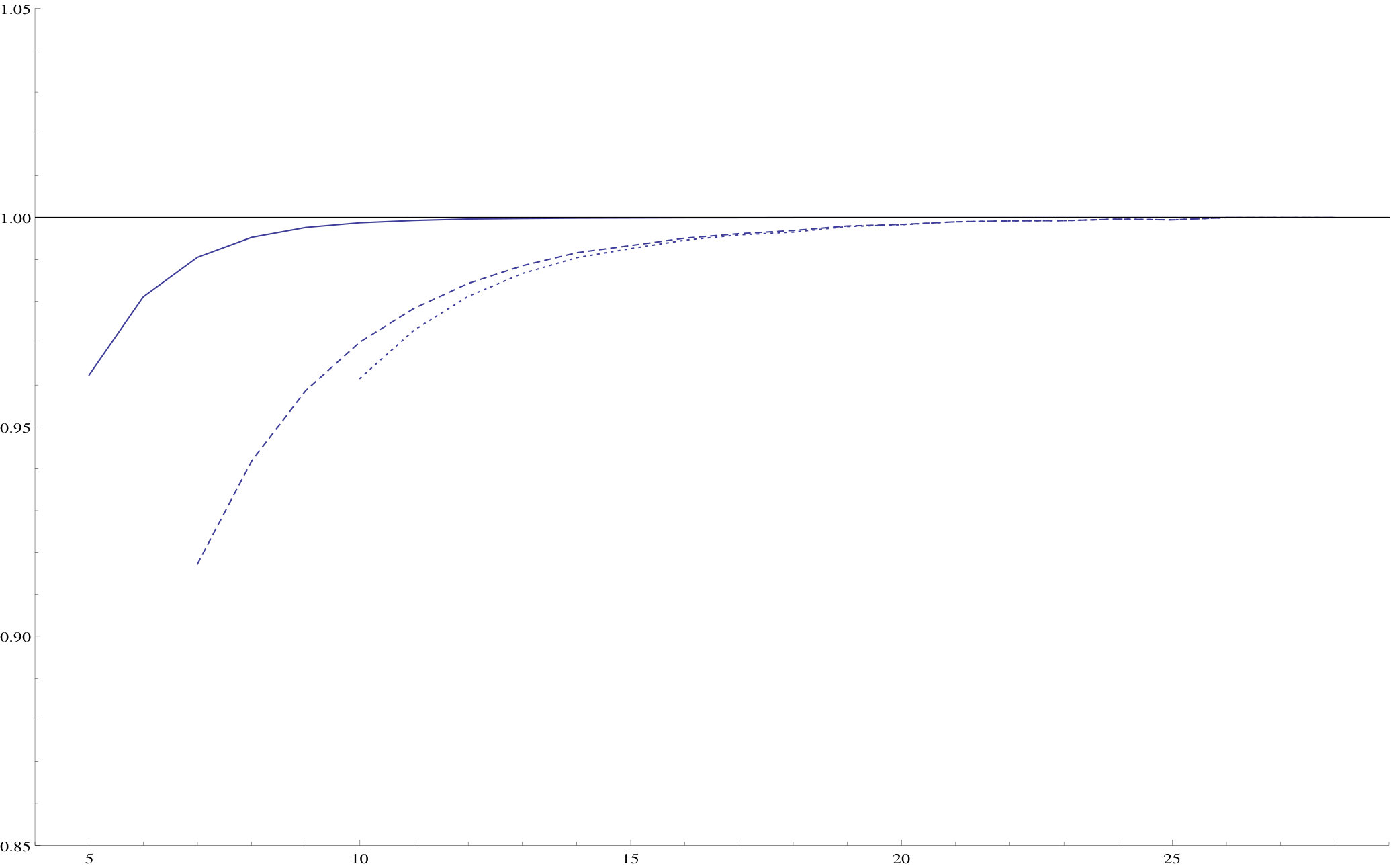 Figure 2
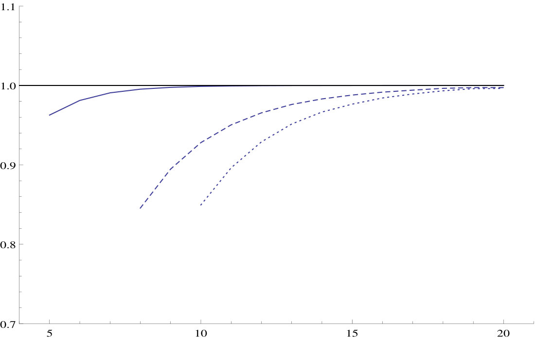 Figure 3
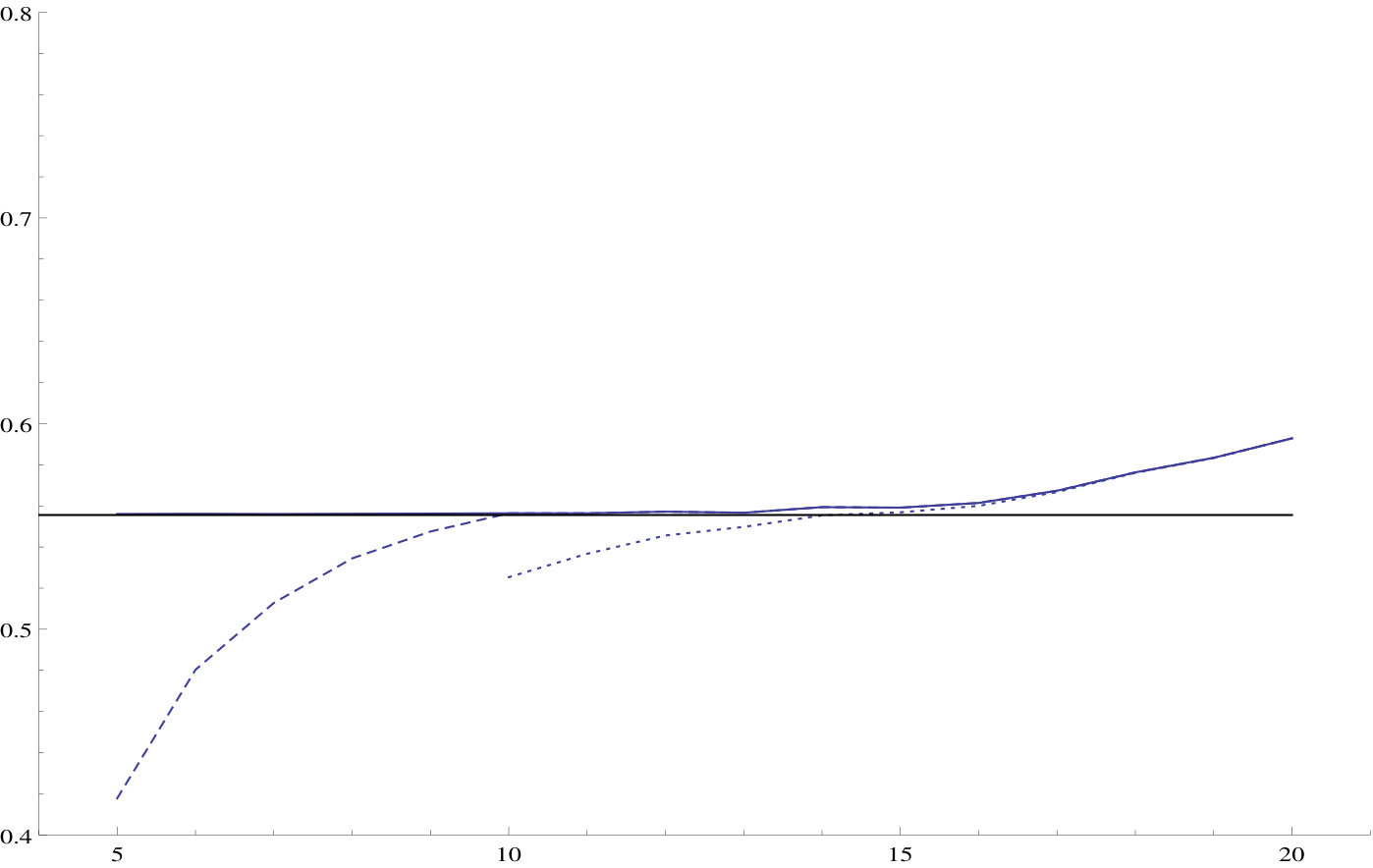 Figure 4
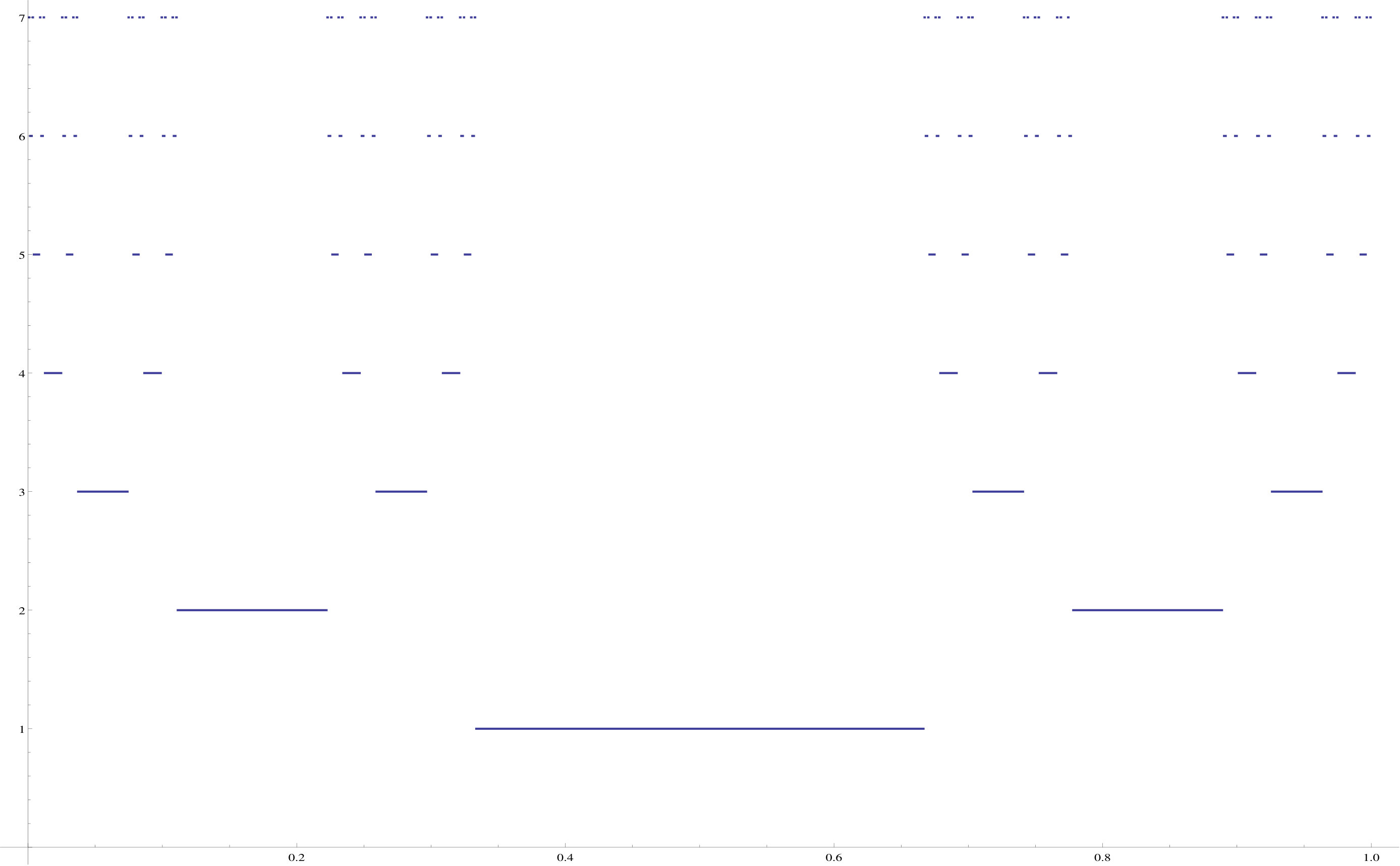 Figure 5
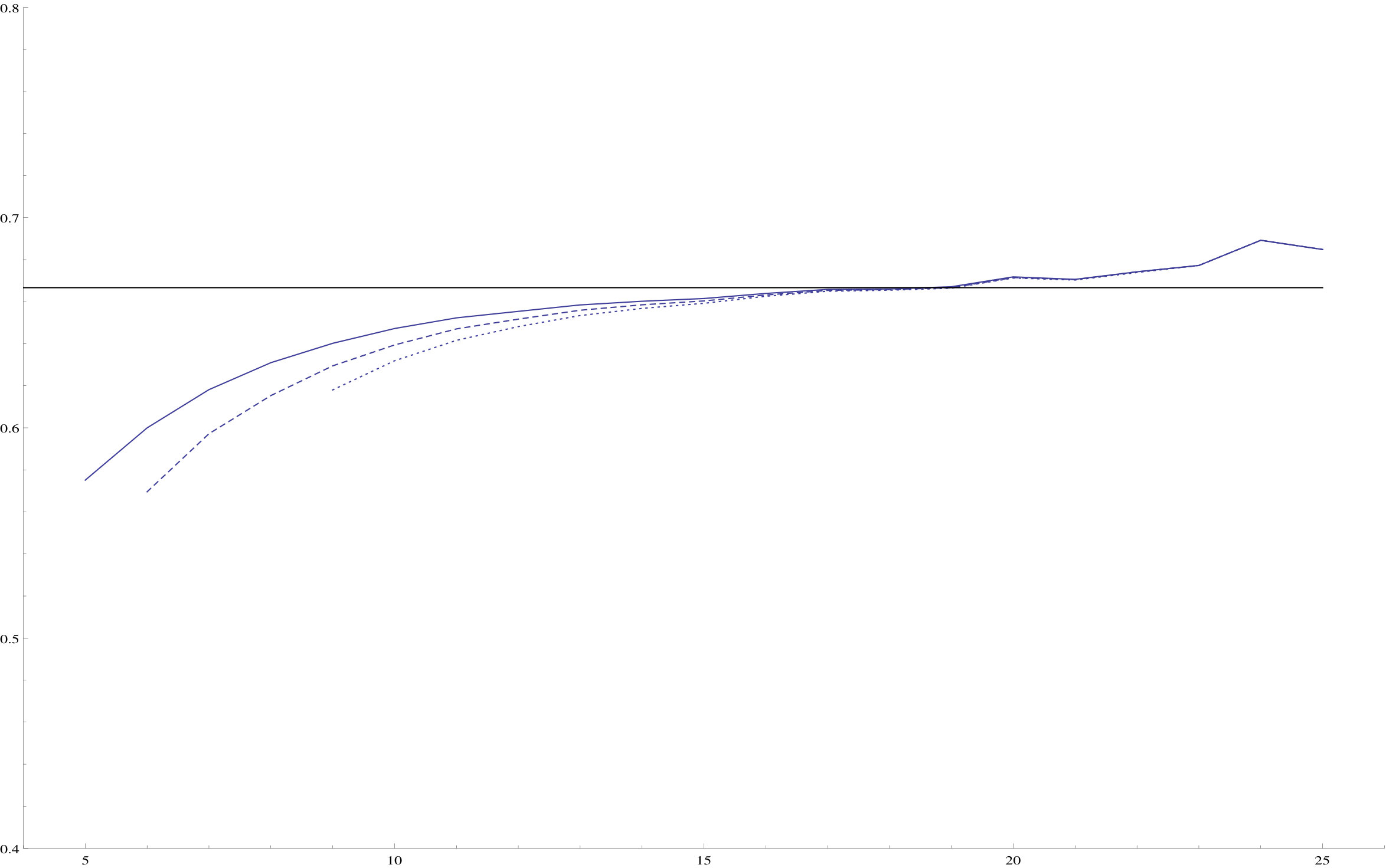 Figure 6
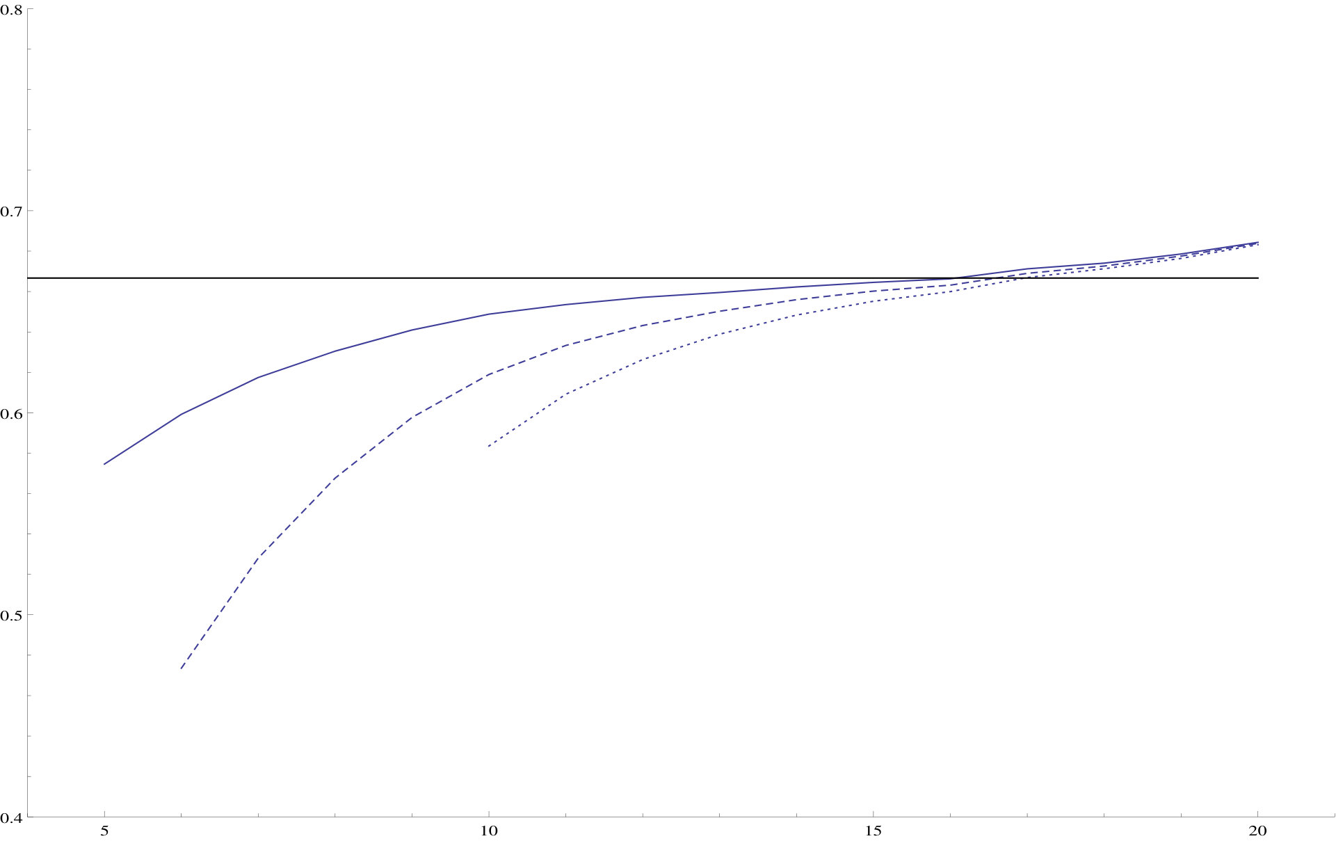 Figure 7
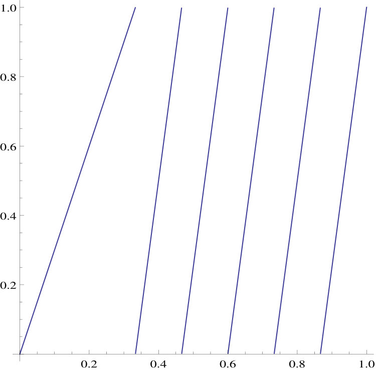 Figure 8
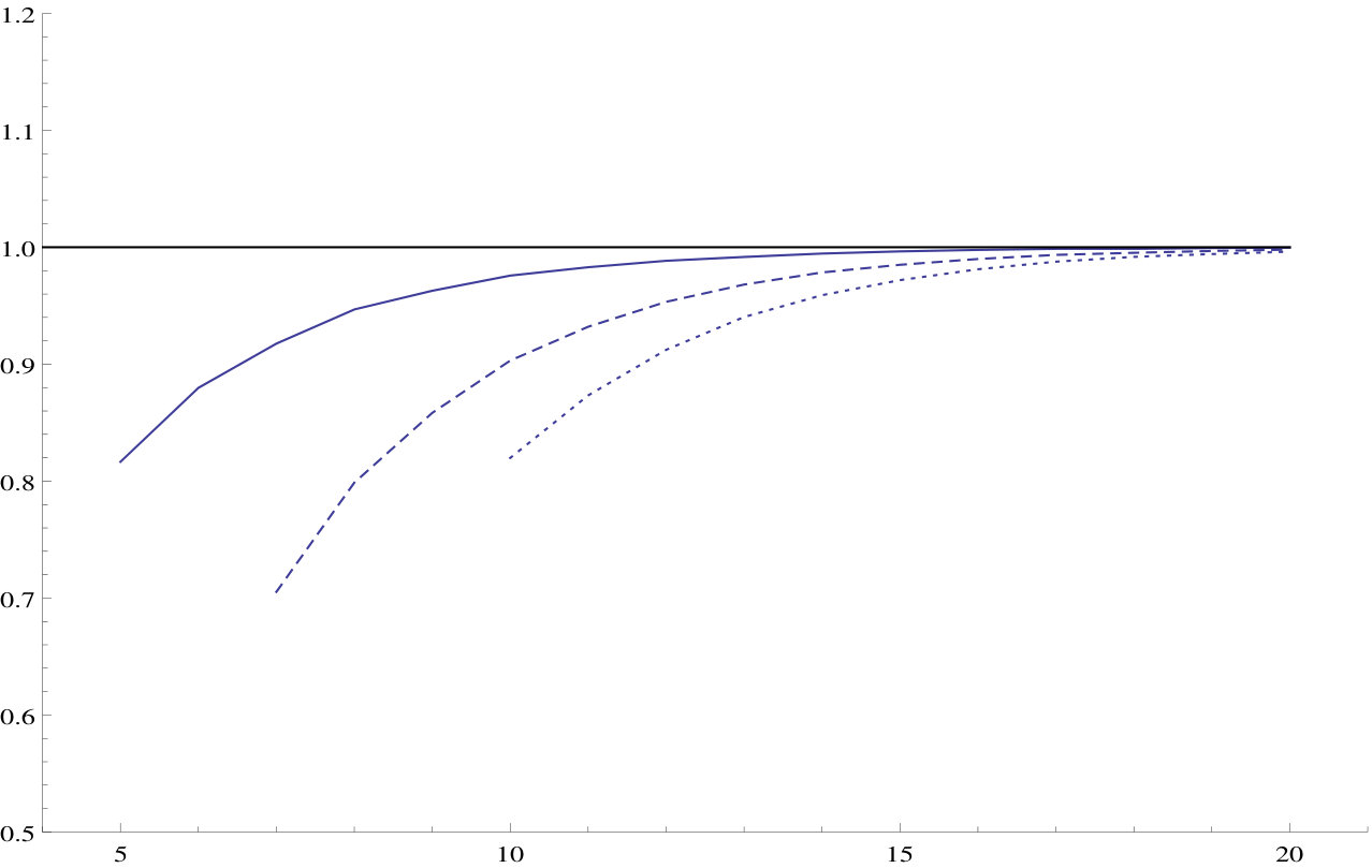 Figure 9
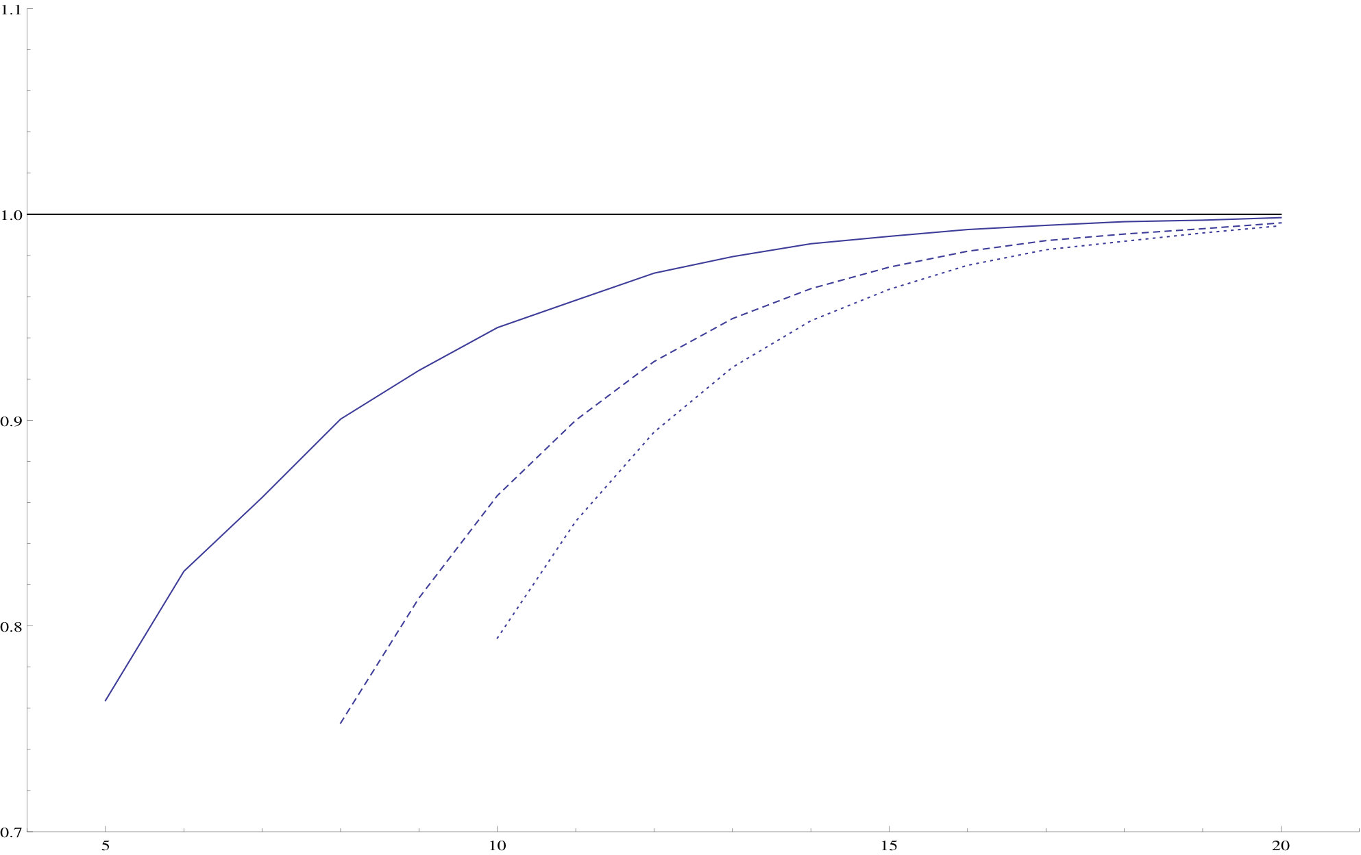 Figure 10
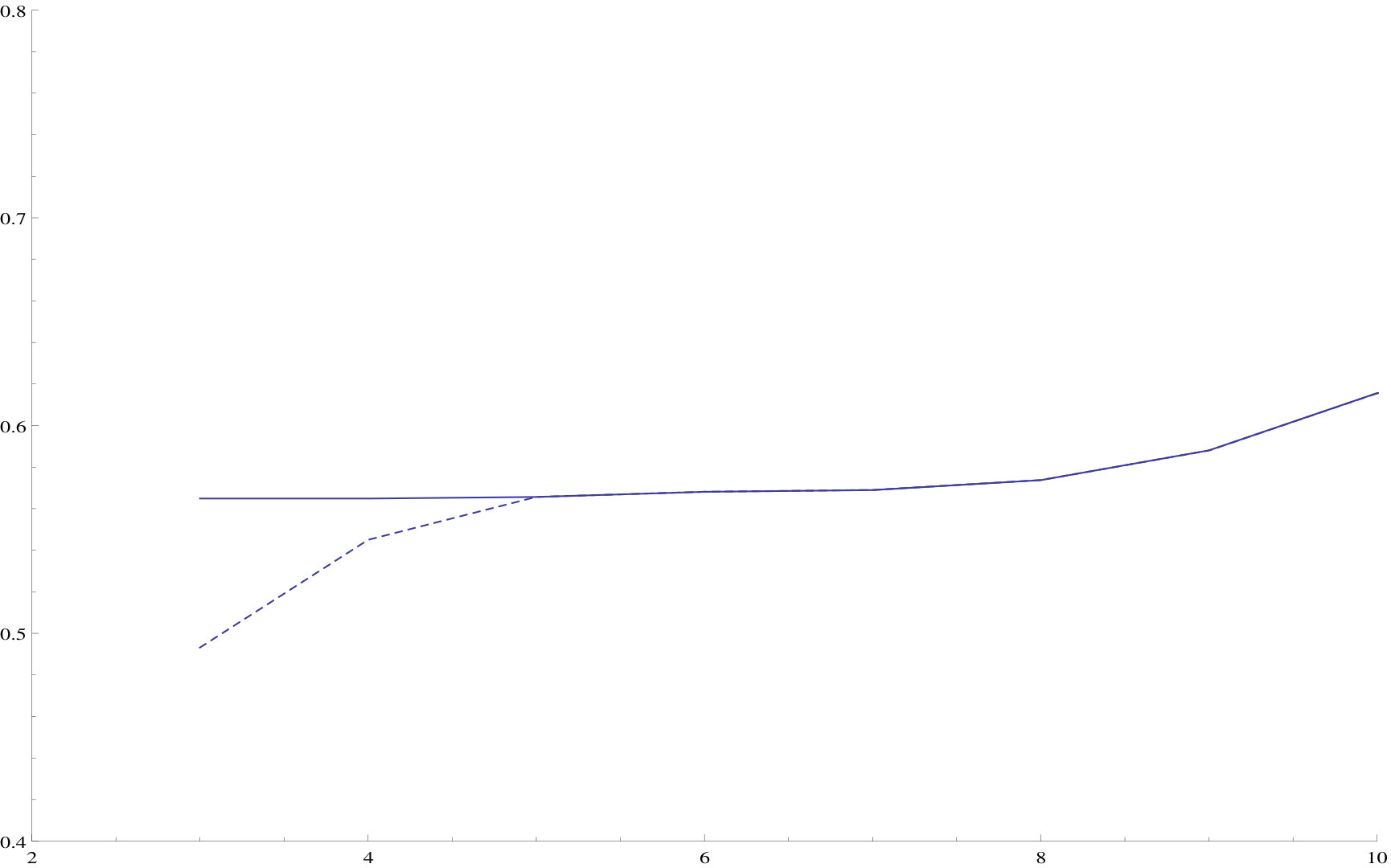 Figure 11
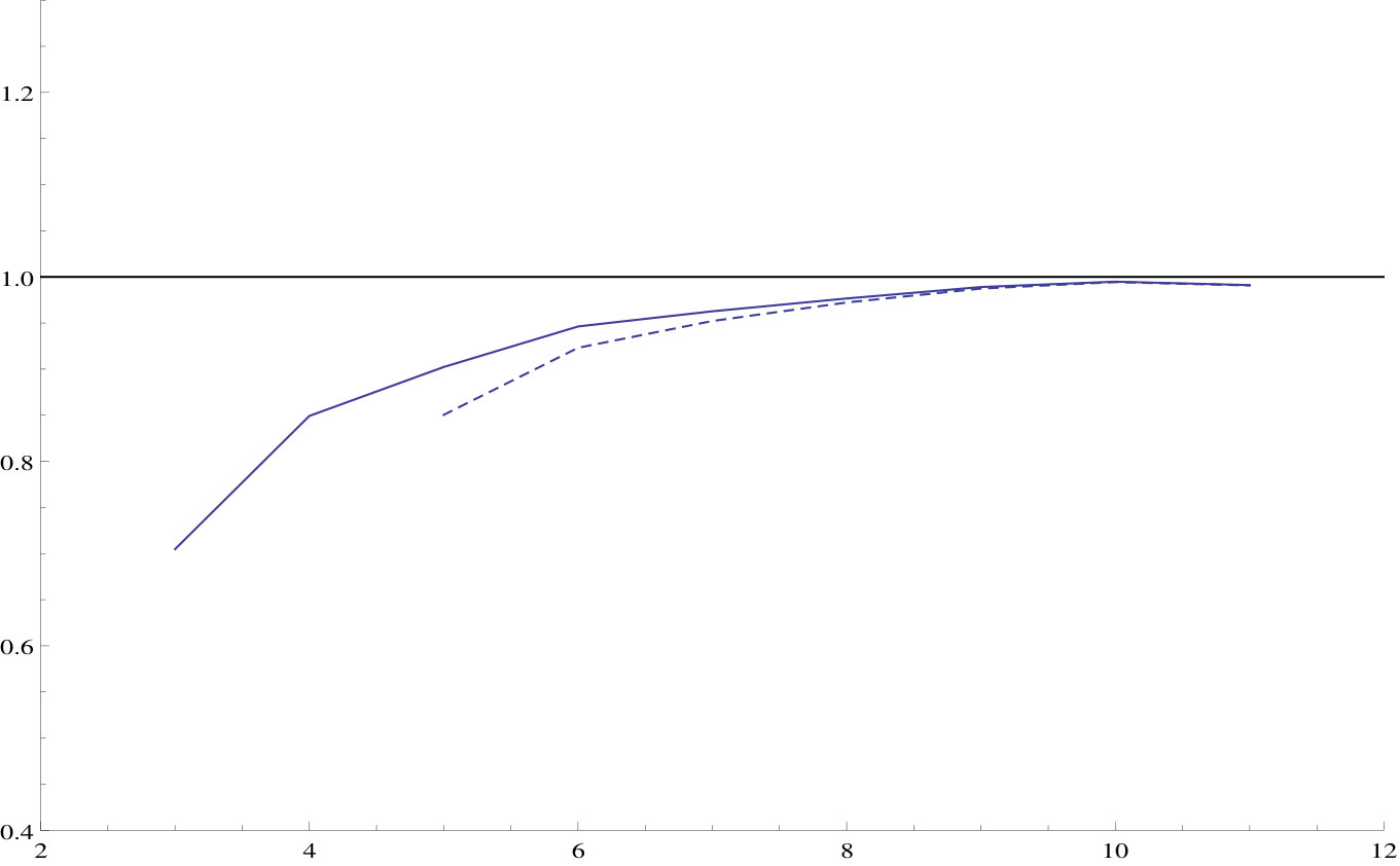 Figure 12
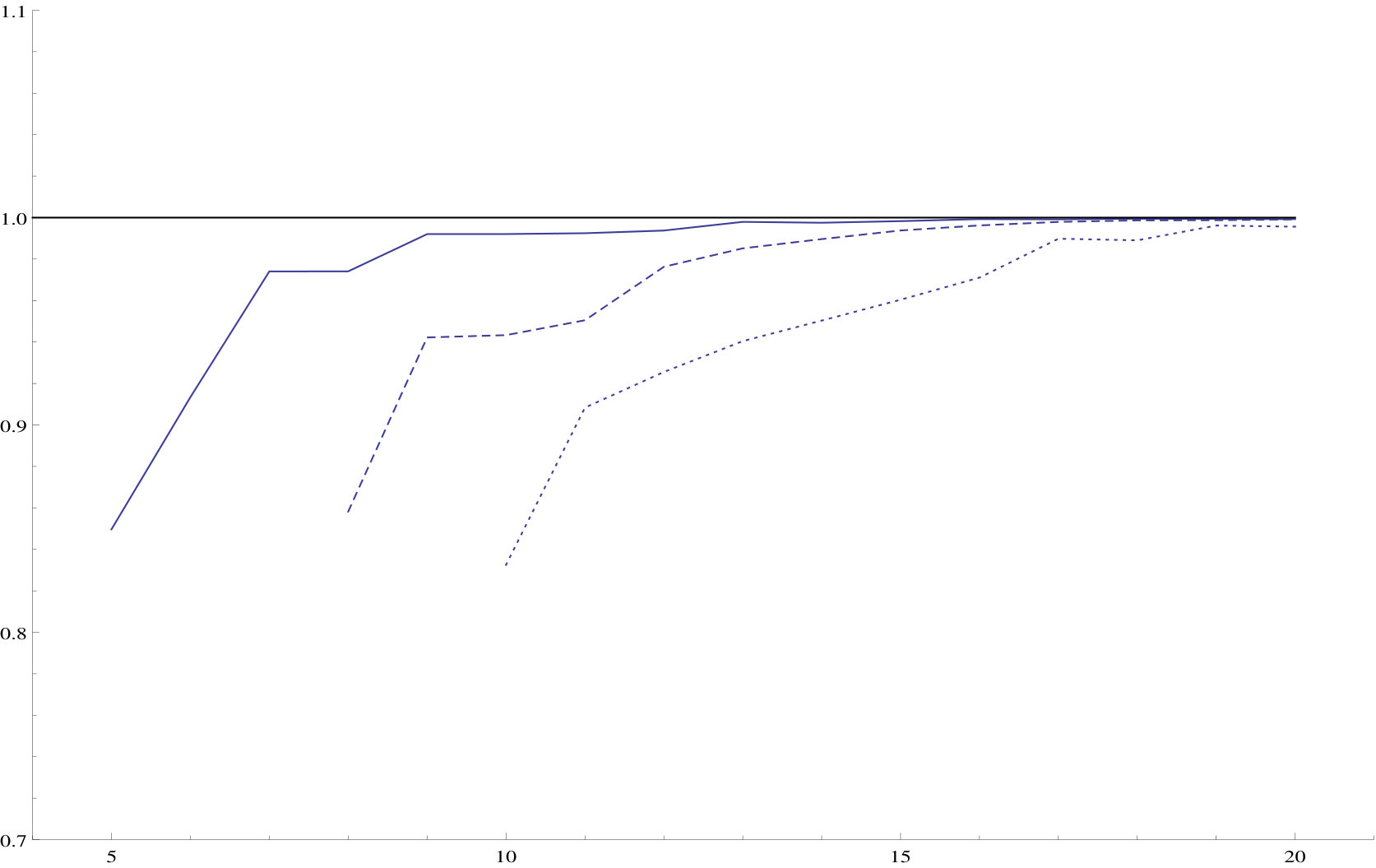 Figure 13
Peer Reviews
No public reviews on file for this paper yet. If you reviewed it on a platform where reviews are public (OpenReview, ICLR, NeurIPS, ICML), you can paste yours below so the community can read it here.
Videos
No videos yet. Explain this paper in a talk, walkthrough, or lecture? Add one.
Rare events for Cantor target sets
Ana Cristina Moreira Freitas
Ana Cristina Moreira Freitas
Centro de Matemática & Faculdade de Economia da Universidade do Porto
Rua Dr. Roberto Frias
4200-464 Porto
Portugal
[email protected] http://www.fep.up.pt/docentes/amoreira/ ,
Jorge Milhazes Freitas
Jorge Milhazes Freitas
Centro de Matemática & Faculdade de Ciências da Universidade do Porto
Rua do Campo Alegre 687
4169-007 Porto
Portugal
[email protected] http://www.fc.up.pt/pessoas/jmfreita/ ,
Fagner B. Rodrigues
Fagner Bernardini Rodrigues
Instituto de Matemática - Universidade Federal do Rio Grande do Sul
Av. Bento Gonçalves, 9500 - Prédio 43-111 - Agronomia
Caixa Postal 15080 91509-900 Porto Alegre - RS - Brasil
and
Jorge Valentim Soares
Jorge Valentim Soares
Centro de Matemática & Faculdade de Ciências da Universidade do Porto
Rua do Campo Alegre 687
4169-007 Porto
Portugal
Abstract.
We study the existence of limiting laws of rare events corresponding to the entrance of the orbits on certain target sets in the phase space. The limiting laws are obtained when the target sets shrink to a Cantor set of zero Lebesgue measure. We consider both the presence and absence of clustering, which is detected by the Extremal Index, which turns out to be very useful to identify the compatibility between the dynamics and the fractal structure of the limiting Cantor set. The computation of the Extremal Index is connected to the box dimension of the intersection between the Cantor set and its iterates.
2000 Mathematics Subject Classification:
37A50, 37B20, 60G70
All authors were partially supported by FCT projects FAPESP/19805/2014, PTDC/MAT-CAL/3884/2014 and PTDC/MAT-PUR/28177/2017, with national funds, and by CMUP (UID/MAT/00144/2019), which is funded by FCT with national (MCTES) and European structural funds through the programs FEDER, under the partnership agreement PT2020. We thank Vuksan Mijović, Mike Todd and Romain Aimino for helpful comments and suggestions.
1. Introduction
The study of rare events for dynamical systems has experienced a vast development in the last two decades (see the book [24] and the review paper [34]) and motivated, in particular, applications to climate dynamics (see for example [35, 30, 29, 7]). The occurrence of rare events is tied to the entrance of the orbit in a sensitive region of the phase space, with small measure, which justifies the use of the word rare. There are two main approaches to the subject: one is through the study of the distribution of the normalised elapsed time that the orbits take to hit or return to such regions of the phase space, which we will refer to the study of Hitting/Return Times Statistics (HTS/RTS), and the other is through the study of the extremal behaviour (distribution of the maximum) of stochastic processes arising from the system simply by evaluating a given observable through the orbits of the system.
The two approaches were proved to be equivalent [9, 16, 17], when the points where the observable function exceeds a high threshold correspond exactly to the sensitive region, which is used for target set for the study of HTS/RTS. Then the underlying idea is that the stochastic process showing no exceedances of a certain high threshold up to time means that the hitting/return time to the respective target set must be larger than . The limiting laws are obtained when the threshold increases to its maximum value, which means that the target sets shrink to the maximal set, , where the observable function achieves its global maximum value.
In the existing literature regarding the study of rare events for dynamical systems (in both approaches), most of the times, the set is reduced to a single point. However, in a few papers, has been chosen to be a finite set of points ([20, 3]), a countable set ([4]), a one dimensional submanifold, such as the diagonal of product spaces ([8, 23, 14]), but has always been taken with a regular geometric structure. The exception is the paper [26], which served as motivation for the present work, where the authors consider the situation of fractal landscapes, with taken as a Cantor set. They conjectured that the same distributional limits observed when was a singular point should apply for such more intricate maximal sets. Their contribution can be described, in their own words, as experimental mathematics: while the definitions of the objects under examination, as well as the form of the conjectured limiting laws, were complete and rigorous and, most of the times, the value of various constants involved were obtained from explicit computations, they did not provide proofs of the conjectured results, which were supported by numerical simulation studies. Their study also revealed the importance played by the Minkowski dimension and Minkowski content in the choice of the normalising sequences in order to recover the classical distributional limits.
The motivation to use maximal sets with a finer geometrical structure comes from the possibility of applications to real life situations when one has many variables and the sensitive regions of the phase space are described as fractal landscapes. Cases such as mine swiping, the movement of air masses, road traffic, network communications, structural safety, stock market, where one is particularly worried with the occurrence of certain critical configurations that correspond to sensitive regions with a complex structure, are very common in the real world. Therefore, understanding the extremal dynamics of simpler lower dimensional models, but which still capture the landscape fractal complexity of the critical regions, is of the utmost importance.
Hence, in this work we assume that is a Cantor set and prove that the conjectured limit behaviour observed in [26] holds true for uniformly expanding dynamics. To our knowledge, this is the first time that rare events limiting laws are proved analytically for a limiting target set (or maximal set) with a fractal geometry. Moreover, we study the possibility of occurring clustering of extreme events for such maximal sets. We remark that, in all the examples considered in [26], with fractal maximal sets with Hausdorff dimension strictly larger than 0, clustering was not detected. Here, not only do we provide examples which show that clustering can still occur in such situations, as we explain the mechanism responsible for the appearance of clustering, by using tools from fractal geometry.
As shown in [18, 3], clustering of rare events is connected with the recurrence properties of by the system’s dynamics. Of course that, when is reduced to a single point, then clustering is related to the periodicity of that point. In fact, in [18, 22, 15, 2, 19], a dichotomy was proved for uniformly and non-uniformly hyperbolic systems: either the single point of is periodic and we have clustering, or is non-periodic and we have the absence of clustering. When has finitely many or countably many points, as shown in [3, 4], then either the orbits of those points collide with creating clustering or they do not hit and in that case, as observed also in [20], there is no clustering. This explains the detection of clustering in the last example of [26], where was a countable set of points.
The presence of clustering is detected by the Extremal Index (EI), which is a parameter that takes values between 0 and 1 and appears as an exponent in the usual exponential limiting law. When there is no clustering the EI is equal to 1, while the presence of clustering leads to an EI less than 1. The more intense is the clustering the smaller is the EI.
As seen in [18, 3], for a nice discrete time system , when is finite then an EI less than 1 implies that the orbits of the points of hit the maximal set itself, i.e., there exists some such that . When dealing with an infinite but countable extremal set , typically, a fast recurrence from to itself produces an EI less than 1, as in the finite case. Nevertheless, in some special cases like [4, Example 4.7], a very slow recurrence of the orbits of the maximal points to may turn the clustering negligible so that in the limit the EI is still 1. We will see that when is uncountable the situation is more complex and the value of the EI is linked to the finer geometrical properties of , namely, to its fractal dimension and thickness.
We will see (Sections 3 and 6) that one may have a large and fast recurrence of the orbits of the points of to itself, i.e., the set may be even infinite for small , and yet the EI is still 1. In the context of Theorems 3.2 and 3.3, the EI will only be less than 1 if one of the intersections , for , is relevant in the sense that its box dimension is equal to the box dimension of , otherwise we will always get an EI equal to 1. Hence, the EI indicates how the dynamics of is or is not compatible with the geometric structure of .
We will illustrate this behaviour analytically with simple models and dynamics, namely, in Section 3, the maximal set will be the ternary Cantor set and will be a uniformly expanding map of the form , with . This simplification allows to compute concrete estimates for the box dimension of the intersections mentioned earlier and exact values for the EI. In the case of presence of clustering created by a clear compatibility between the dynamics and the self-similarity structure of the maximal set, we will consider more general Cantor sets (see Section 4). We remark that although we work with simple models, they capture the essence of the limiting behaviour of the statistics of rare events dynamics and, in fact, we believe that the spirit of our findings should prevail in more irregular situations, as the numerical simulation study performed in Section 6 suggests.
As seen in [25], the authors considered reduced to a single point chosen in the support of a dynamical attractor and have shown that extremes can be thought of as geometric indicators of the local properties of the attractor. Here, is an intricate, much more general set, which means that the extremes, instead of a local information provide a global one. In fact, we believe that an interesting byproduct of our results is that the EI could be used as an indicator of the compatibility of a certain dynamics with the geometric self-similarity structure of . Namely, in the cases considered, we obtained that the EI is always 1, except for the cases when for some , which are precisely the maps that have as an invariant set.
The dimension of the intersection of fractal sets such as Cantor sets is an important problem popularised by some of Furstenberg’s conjectures, which in particular state that “expansions in multiplicatively independent bases (such as 2 and 3) should have no common structure”. We refer to [36] and references therein. In order to illustrate the potential of the EI as an indicator for the relevance of the intersection of fractal sets and the compatibility of a certain dynamics with the self-similar structure of a Cantor set, we used an estimator of the EI, introduced in [21], and carried out a numerical study in order to demonstrate its performance by comparing with our theoretical estimates.
The paper is structured as follows. In Section 2, we introduce the framework regarding the study of rare events for dynamical systems and state general results providing conditions in order to obtain the existence of limiting laws. In Section 3, we introduce the observables maximised on Cantor sets (the ternary Cantor set, to be more precise), define the dynamical models and state the main results of the paper. In Section 4, we state a general theorem establishing the existence of a limiting law, in the presence of clustering, for general dynamically defined Cantor sets and compatible dynamics, which allows to prove one of the main theorems stated in the previous section. In Section 5, we prove the other main theorem stated in Section 3 regarding the existence of a limiting extreme value law, in the absence of clustering. This is the more elaborate part and includes a brief review of several tools of fractal geometry. In Section 6, we present a numerical simulation study to illustrate the suitability of the use of the EI as an indicator of the compatibility between the dynamics and the geometrical fractal structure of the maximal set.
2. Laws of extreme events
Consider a discrete dynamical system , where is a compact set (an interval, in our case), is the respective Borel sigma algebra, is a measurable map, and is an invariant measure with respect to . We will follow the Extreme Value approach and, therefore, we consider an observable function and define the stochastic process, , in the following way,
[TABLE]
Note that the invariance of implies the stationarity of . We are particularly interested in the extremal behaviour of such stochastic processes, which is tied to the recurrence properties of the set of global maxima of , as was proved in [16, 17]. We denote this set of global maximal points as , i.e., we assume that there exists , where we allow , and
[TABLE]
In what follows, will always denote a generic point of . In this paper, most of the times, , where denotes the usual ternary Cantor set.
From the stochastic process , we define the process of partial maxima whose limiting distribution we want to analyse:
[TABLE]
In order to study the extremal behaviour of , we consider the level sets , i.e., the exceedances of a high threshold , which correspond to the target sets in the HTS/RTS approach, and try to obtain a limit for the probability of not observing any exceedance up to a certain moment of time , which depends on the level . More precisely, we want to estimate as or, in other words, when the target sets shrink to . In order to obtain a non degenerate limit, the dependence of on must be well tuned.
When as a function of is not smooth, as happens here, this tuning must be performed with some care and we will use the normalisation introduced in [17] to deal with similar cases. Namely, we consider sequences and such that
[TABLE]
Then our main goal is to find some non-degenerate distribution function supported on such that
[TABLE]
In [17] this type of distributional limit was called cylinder Extreme Value Law (EVL). When is a finite or countable set of points and is either a uniformly expanding map or admits an hyperbolic first return time induced map, then, as seen for example in [18, 22, 20, 2, 19, 3, 4], we have that
[TABLE]
where . When such a limit exists, then is called the Extremal Index. The EI is associated to the recurrence properties of . In fact, when is reduced to a single point, as seen in [18, 22, 2, 19], a full dichotomy holds: either is non-recurrent, which translates to being non-periodic, and then there is no clustering of exceedances and , or is recurrent, i.e., is a periodic point, which is responsible for the appearance of clustering and an EI less than 1 (if the map is differentiable along the orbit of and the invariant measure is absolutely continuous w.r.t. Lebesgue measure, we have ).
2.1. Existence of limiting laws
The main purpose of this subsection is to provide general conditions which allow us to prove the existence of a limiting law as stated in (2.4). Let and be as in (2.3). Consider a sequence such that
[TABLE]
Let denote the -th preimage by the map . Fixing and , we define the following events,
[TABLE]
While the event corresponds to the occurrence of an exceedance, the event corresponds to the occurrence of an exceedance which terminates a cluster of exceedances, i.e., if occurs, then the next exceedance after the one observed at time must belong to a new and different cluster of exceedances. In particular, can be though as the maximal waiting time between two exceedences within the same cluster.
Let be an event. For , we define,
[TABLE]
Observe that For each , set , and
[TABLE]
We will see that provides a good estimate for the EI. In fact, the EI, , will be such that
[TABLE]
We will refer to (2.8) as O’Brien’s formula to compute the EI (see [32]).
We start by stating a condition that requires some sort of asymptotic independence of events when the time gap between them increases.
Condition** ().**
We say that holds for the stochastic process if for every
[TABLE]
where is decreasing in for each and there exists a sequence such that and when .
The next condition forbids the concentration of clusters of exceedances. Consider the sequence given by condition and let be another sequence of integers such that
[TABLE]
Condition** ().**
We say that holds for the sequence if there exists a sequence satisfying (2.10) such that
[TABLE]
We can now state a general result establishing the existence of a limiting extreme value law.
Theorem 2.1**.**
Let be a stochastic process constructed as in (2.1). Consider the sequences and satisfying (2.3) for some . Assume that conditions and hold for some satisfying (2.5). Moreover, assume that the sequence defined in (2.7) converges to some , i.e., . Then,
[TABLE]
The proof of this theorem follows from an easy adjustment of the proof of [24, Corollary 4.1.7].
2.2. Applications to systems with loss of memory
One of the main advantages of the previous conditions when compared with the usual ones from the classical Extreme Value Theory is that is easily checked for systems with nice decay of correlations, while the classical conditions of the kind, similar to Leadbetter’s condition, require a uniform mixing which is very difficult to verify even for hyperbolic systems.
Definition 2.2** (Decay of correlations).**
Let denote Banach spaces of real valued measurable functions defined on . We denote the correlation of non-zero functions and with respect to a measure as
[TABLE]
We say that the dynamical sytem has decay of correlations, with respect to the measure , for observables in against observables in if there exists a rate function , with
[TABLE]
such that, for every and every , we have
[TABLE]
The systems we will work with have decay of correlations of functions of Bounded Variation, which we define below, against observables in .
Definition 2.3**.**
Given a potential on an interval , the variation of is defined as
[TABLE]
where the supremum is taken over all finite ordered sequences .
We use the norm , which makes the space of functions of Bounded Variation, , into a Banach space.
We will see that conditions and follow from the above mentioned type of decay of correlations of the underlying dynamical system.
Theorem 2.4**.**
Let be a dynamical system and consider an observable achieving a global maximum on a set . Let be the stochastic process given by (2.1) and consider , and as sequences such that (2.3) and (2.5) hold. If the system has decay of correlations of observables in against observables in and if
- (1)
, for some sequence such that 2. (2)
**
and if the sequence defined in (2.7) converges to some , then conditions and are satisfied and
[TABLE]
Remark 2.5**.**
Note that under the assumption of summable decay of correlations against then hypothesis (1) implies , while hypothesis (2) implies .
Proof.
By Theorem 2.1, we only need to check that the stochastic process satisfies conditions and .
Consider and in Definition 2.2. Then, there exists , such that, for any positive numbers and , we have
[TABLE]
Condition follows if there exists a sequence such that and , which is the content of hypothesis (1).
In order to prove (2.11), we start by observing that
[TABLE]
Then, we take , in Definition 2.2, to obtain that
[TABLE]
Let be as above and take as in (2.10). Recalling that , it follows that
[TABLE]
by choice of and hypothesis (2). ∎
3. Observables with fractal maximal sets
Let denote the ternary Cantor set. In order to construct , we start by removing the middle third of the interval and define in this way the first approximation . Then, we start an iterative process where we build by removing the middle third of each connected component of , as represented in Figure 1. Repeating this process indefinitely, we obtain the set .
We define the observable to be the Cantor ladder function also used in [26] as a prototype fractal landscape. Namely, for each , let so that , , i.e., the sets correspond to the gaps of the Cantor set formed at the -th step of its construction. Now consider the observable
[TABLE]
Remark 3.1**.**
Note that if then for all , which implies that . If then for some and therefore, in this case, we have that .
In this section, we will consider dynamical systems given by:
[TABLE]
where . These are full branched uniformly expanding maps, which preserve Lebesgue measure (that we shall denote by ) and have exponential decay of correlations of BV observables against (this follows from [6, Corollary 8.3.1] or [1, Corollary H], for example).
In [26, Section 3], the authors considered the same observable defined in (3.1) and the dynamics generated by an asymmetric tent map, which is also a full branched uniformly hyperbolic map, and conjectured the existence of a limiting extreme value law with an EI equal to 1, which was supported by the numerical simulations performed. We prove that when the dynamics considered is not compatible with the self-similar structure of the maximal set (which happens here when for all ) then indeed the conjectured extreme limiting behaviour applies. To our knowledge, these are the first rigorously proved results for observables with fractal maximal sets.
Theorem 3.2**.**
Let be the stochastic process given by (2.1) for a dynamical system defined in (3.2), with for all . Consider a sequence of thresholds such that and a sequence of times such that . Then, condition (2.3) holds and moreover
[TABLE]
The numerical simulations performed in [26, Section 3] also showed that, interestingly, the same limiting laws seem to apply when the dynamics is replaced by that of irrational rotations. The fact that these ergodic maps are not mixing and yet the agreement was still good, lead the authors of [26] to conjecture that the role of the fast decay of correlations in assuring the validity of conditions such as and was played, in this situation, by the complexity of the observable function. We also remark that, in all numerical studies performed in [26] with observables maximised on fractal sets (with strictly positive Hausdorff dimension), the observed EI was always 1. In our results we use heavily the excellent mixing properties of all the systems considered. However, not only we provide examples where the EI is strictly less than 1, as we explain how the EI is related with the compatibility between the dynamics and the fractal structure of the maximal set.
Theorem 3.3**.**
Let be the stochastic process given by (2.1) for a dynamical system defined in (3.2), with for some . Consider a sequence of thresholds such that and a sequence of times such that . Then, condition (2.3) holds and moreover
[TABLE]
In fact, in Section 4, we prove Theorem 3.3 as a corollary of Theorem 4.2 which applies to more general Cantor sets. We note that, in the context of both Theorems 3.3 and 4.2, the compatibility between the dynamics and the maximal set becomes obvious when we observe that , which means that preserves the structure of the Cantor sets, which play the role of a periodic point in the context of when is reduced to a single point. The proof will follow more or less the same strategy used in [18] and generalised later in [3, 4], which basically exploits the periodicity of the maximal set in order to be able to compute the EI from the O’Brien’s formula (2.8) and then verify the conditions and that were designed to be easily checked from the excellent mixing properties of the system.
When for all , although for all , one can easily check that, most of the times, we have that and this was enough to create clustering when was a finite or countable set (see [3, 4]). However, here, the maximal set has a much more complex structure and one needs to evaluate how relevant the intersections are when compared with itself, which translates to how compatible the dynamics of is with the fractal structure of . We will see that since has a thickness not less than 1 (i.e., the extractions in the construction of the Cantor set are relatively not too large), then the relevance of the intersection (or the compatibility between and ) can be measured by the box dimension of the intersection , when compared with the box dimension of itself. We will show that the box dimension of is strictly less than that of (Proposition 5.8), which means that the possible clustering created by the fact that is negligible and, in the limit, the EI is still 1. The computation of the EI is much more subtle and we need results from fractal geometry in order to compute the dimension of such intersections and then we need to study its impact on O’Brien’s formula (2.8), for which we will perform a finer analysis, where we use of the notion of thickness of dynamically defined Cantor sets introduced by Newhouse in [31]. This will be done in Section 5.
4. The appearance of clustering with fractal landscapes
When the dynamics is compatible with the self-similar structure of the fractal maximal set, we observe the appearance of clustering and a limiting law with a non-trivial EI. In this context, we consider more general fractal sets. Namely, we will consider Cantor sets generated by an Iterated Function System (IFS) satisfying some regular conditions. These Cantor sets can also be identified as the survivor sets for some conveniently chosen dynamical systems, which will also provide a common ground to assess the compatibility of the self-similarity structure with the original dynamics. We will start by providing a description of these more general dynamically defined Cantor sets. Then, we establish the existence of a limiting law with a non-trivial EI when the dynamics is compatible with the system generating the Cantor set and, finally, we apply it to the usual ternary Cantor set.
4.1. Dynamically defined Cantor sets
We start with a description of a class of more general Cantor sets.
Let and be a regular finite family of normalised contractions defined on , i.e., each is a diffeomorphism such that
[TABLE]
and the sets , for , are pairwise disjoint. is in particular an Iterated Function System (IFS). An atractor for is the only compact subset, , of , such that . For such an IFS there exists a unique attractor , whose Hausdorff and box dimensions (see Definitions 5.1 and 5.2 below) are both equal to , where . See [13, Chapter 9] for proofs and more details on the subject. The attractor can be seen as a dynamically defined Cantor set, i.e., can be identified as the survivor set of the dynamical system defined by
[TABLE]
Namely,
[TABLE]
Let and for all set
[TABLE]
Remark 4.1**.**
Note that and, for all , we have because if then for all .
4.2. Laws of rare events for systems compatible with dynamically defined Cantor sets
We adapt the definition of the observable function so that, in this case, the maximal set is . Namely, we set
[TABLE]
Now we define a dynamical system which is compatible with the dynamics that generated , namely, we define by for all and if denotes a connected component of then, on , we define as a linear map so that maps onto . Note that is a piecewise uniformly expanding map and therefore admits an invariant absolutely continuous probability measure . Moreover, from [6, Corollary 8.3.1], it follows that has exponential decay of correlations of BV observables against , i.e., for all and , there exist and such that
[TABLE]
Theorem 4.2**.**
Let be the stochastic process given by (2.1) for the dynamical system , for some , where and the observable are as defined just above. Consider a sequence of thresholds such that , a sequence of times such that .
Assume that there exist a sequence , with , and a sequence , as in (2.5), such that: and .
Assume moreover that there exists such that
[TABLE]
Then,
[TABLE]
Proof.
We start by noting that for the sequence of thresholds , we have and then the definition of makes condition (2.3) trivially satisfied.
Next, we observe that the compatibility between and allows for a simple characterisation of the sets . We claim that
[TABLE]
To check this claim we start by proving that for all , we have
[TABLE]
Clearly, . For the other inclusion, consider that . Since , then for all and since then . Since , then , which means that for all and therefore . Now, observing that for all and recalling the definition of we obtain:
[TABLE]
The fact that has decay of correlations of BV against as expressed in (4.1) together with the assumptions and guarantee that conditions (1) and (2) from Theorem 2.4 hold. Moreover, the assumption on gives that . Consequently, the result follows from direct application of Theorem 2.4. ∎
4.3. Application to the ternary Cantor set
We apply Theorem 4.2 to the ternary Cantor and prove Theorem 3.3.
Proof of Theorem 3.3.
We start by checking the hypothesis of Theorem 4.2 and then verify the formula provided for the Extremal Index . In this case, the IFS is given by and , the map is given by , the cantor set and . The invariant measure is Lebesgue measure and the rate of decay of correlations expressed in (4.1) is such that . We set and observe that and . Since , for all , and , then , and we obtain:
[TABLE]
and, moreover,
[TABLE]
Let and note that clearly . Since , then
[TABLE]
Moreover, there exists some constant, , such that
[TABLE]
Finally, we use O’Brien’s formula to compute the EI:
[TABLE]
As a consequence of Theorem 4.2, we obtain ∎
5. The absence of clustering for fractal maximal sets
As we mentioned earlier, when there is no compatibility between the dynamics and the self similarity structure of the fractal maximal set, then no clustering of rare events is expected. This compatibility is related to the significance of the intersections between the maximal set and its iterates. The significance will be measured by the box dimension of those intersections and therefore we start in Section 5.1 by recalling some techniques that we will use in order to estimate the dimension of the referred intersections, which will be carried out in Section 5.2. Then, in Section 5.3, we translate the significance of the intersection expressed in terms of box-dimension into the relevance of the measure of when compared with the measure of . This will be done using the notion of thickness used by Newhouse in [31]. Finally, in Section 5.4, we prove conditions and , in order to conclude the proof of Theorem 3.2.
5.1. Preliminaries and notions from Fractal Geometry
One of the main difficulties to prove the existence of extreme value laws for stochastic processes arising from observables maximised on Cantor sets is to calculate the EI based on O’Brien’s formula. In the next sections, we will present a technique to calculate the EI based on the box dimension of the sets . To do this, we will need a construction given in [28], where the author uses Digraph Iterated Function Systems, introduced in [27], in order to describe the intersection of fractal sets. Then, we will combine a result from [27] to estimate the Hausdorff dimension of such intersections with a result from [10], which relates the respective Hausdorff and box dimensions, so that we obtain an estimate for the box dimension of the intersections , which we will, ultimately, use later to compute the EI.
We start by recalling some notions of Fractal Geometry (referring to the book [13] for further details) and, in particular, the concept of Digraph Iterated Function System used by McClure to describe the intersection of fractal sets in [28].
Definition 5.1** (Box Dimension).**
Let be a subset of , then, the box dimension of is defined as
[TABLE]
where denotes the smallest number of balls of radius that cover , whenever the limit exists. The upper and lower box dimension are defined by taking the and , respectively, in the previous limit.
Definition 5.2** (Hausdorff Dimension).**
Let be a subset of and be a countable collection of sets, with diameter at most , that cover . For , we define the - dimensional Hausdorff measure of as
[TABLE]
The Hausdorff dimension of is defined as
[TABLE]
Both definitions of dimension are finitely stable, i.e., if is a finite collection of subsets of , then
[TABLE]
Remark 5.3**.**
We note that the box dimension of the ternary Cantor set is . Moreover, since can be generated from an Iterated Function System (IFS), which satisfies the so called open set condition, then the box dimension of coincides with its Hausdorff dimension. We defer to [13] for definitions and proofs of these statements.
The notion of Digraph Iterated Function Systems (Digraph IFS) generalizes the most common setup of IFS. We follow closely the notation and presentation in [28].
Definition 5.4** (Digraph IFS).**
A Digraph IFS consists of a digraph where the set of vertices is denoted by and the set of edges is denoted by . To each of the vertices, we associate a metric space . Furthermore, to each of the edges between two vertices and , denoted by , we associate a similarity with ratio . For every path in the graph , we form the function by composing the functions along the path in reverse order. The ratio of is just the product of the ratios of the composed functions. If every is less than one, then, there exists a set, , which is a union of compact sets , one for every vertex, such that for every ,
[TABLE]
This invariant set, , is called the attractor of the Digraph IFS. The existence of this set is guaranteed if the similarities have ratios smaller than one (see [12]).
It is possible to represent a Digraph IFS in matrix notation. For that purpose, we construct a Digraph IFS matrix, , with entries indexed by . The value of each entry will be the set of edges that link one vertex to another. To a Digraph IFS, , we also associate a Digraph IFS substitution matrix, , which is just the adjacency matrix of digraph .
If is an attractor of a standard IFS and is a bijection, then can be represented as an attractor of a Digraph IFS. Namely,
Theorem 5.5** (Theorem 1 of [28]).**
Let be an attractor of an IFS, , such that all functions are bijective contractions. Assume that there exists a finite set of bijections, , such that, for all satisfying and for all satisfying , then . Under this condition the list of sets forms the attractor of a Digraph IFS.
In order to construct the Digraph IFS whose attractor is , it is necessary to use an iterative process to find the set of functions . We start with a set , then we define the set
[TABLE]
To fulfil the hypotheses of Theorem 5.5, in each step, we select only those functions, , such that . We continue the procedure until no new function is found. The functions in will work as the vertices of the Digraph IFS while the edges will be labelled by the functions . So, each row and line of the matrix have an associated function that belongs to the set . Each entry of this matrix can be represented by a pair of functions . Each of the entries will be a finite set of functions
[TABLE]
whose cardinality is the number of directed edges from to , where a function belongs to this set if and only if
[TABLE]
for some .
The substitution matrix, , of the Digraph IFS, will be the matrix but with each entry replaced by the cardinality of the corresponding set.
Definition 5.6** (Open Set Condition).**
A Digraph IFS satisfies the open set condition if and only if there exists open sets , such that, for every and ,
[TABLE]
and for all , and with ,
[TABLE]
From [27], one has that the Hausdorff dimension of the attractor of a Digraph IFS satisfying the open set condition (which, by [10], under certain conditions that are verified in our setting, is equal to its box dimension) can be written in terms of the spectral radius of and the common ratios of the similarities of the Digraph IFS. For this reason, we recall here the definition and some useful properties of the spectral radius of a matrix. Let be a complex matrix. The spectral radius of is defined as
[TABLE]
The Euclidean norm of a complex matrix is defined as
[TABLE]
where is the usual Euclidean vector norm. This norm is multiplicative (in some literature also called consistent or sub-multiplicative) in the sense that satisfies for arbitrary matrices and . Moreover, we have (see [11], for example):
[TABLE]
Assume that is a nonnegative matrix, i.e., every entry is either positive or [math]. If is a principal submatrix of , then the spectral radius of satisfies (see [5], for example):
[TABLE]
We end this subsection by stating an inequality that will become very useful later in the estimation of the spectral radius of the adjacency matrix that we will construct.
Proposition 5.7**.**
Let by any positive real numbers and consider . Then,
[TABLE]
5.2. Intersection of Fractal Sets
We will now apply the procedure described in Section 5.1 (see [28, Section 2.2] for further details) to estimate the box dimension of the set . Namely, our main goal is to show:
Proposition 5.8**.**
Let , where for any . Then, for all , we have:
[TABLE]
The rest of this subsection is dedicated to the proof of Proposition 5.8. We start by noting that, for any integer,
[TABLE]
Therefore, the set is a union of sets formed by taking the preimage of by each one of the branches of This implies that the functions of interest to us to start the algorithm described in Theorem 5.5 are of the form
[TABLE]
where is of the form with an integer less than . The algorithm leads to the construction of sets of functions, which we denote by for , depending on the constant term of the function that initiates the algorithm. Each of the sets yields a substitution matrix, , associated with the respective Digraph IFS.
Define the functions , where is either [math] or . This set of functions forms an IFS whose attractor is the ternary Cantor set .
For a given and , the functions that belong to the set , are of the form,
[TABLE]
where already belongs to the set in question. Hence, for to belong to , it is necessary that its constant term satisfies
[TABLE]
Therefore, all the functions in are of the form,
[TABLE]
where .
For better understanding, we divide the characterization of the matrices into the following smaller results.
Lemma 5.9**.**
Let and , then, every entry of the matrix is either [math] or .
Proof.
Fix , and let be a function in . As seen in (5.6), any other function that belongs to the set must be equal to
[TABLE]
where is of the form with . To prove the Lemma, we will need to address two different cases, each with two different possibilities:
- •
If then
- •
If then
- •
If then
- •
If then
For the first case, assume that and . Then, we would obtain
[TABLE]
Since and , we are led to which is an absurd.
Consider that and . Then,
[TABLE]
and , which is an absurd.
Consider that and . Then,
[TABLE]
and which is, again, an absurd.
For last case, assume that and and observe that
[TABLE]
implies , which is an absurd and the Lemma is proved. ∎
Lemma 5.10**.**
Let and , then the sum of the elements of each row of the matrix is at most .
Proof.
Consider a function in . As seen before, any other function must be of the form
[TABLE]
where with . According to the possible values of and there are four different possibilities for the line of indexed by to have entries equal to . We will prove that these cases form two disjoint groups of two elements, which will prove the claim of the Lemma.
Assume that and and that belongs to . By (5.6), the constant term of satisfies
[TABLE]
By contradiction, assume that belongs to with and . Again, by (5.6), the constant term of satifies
[TABLE]
Since is larger than the length of the interval , for any considered, then the two conditions, (5.7) and (5.8), cannot be simultaneously fulfilled for any and the two cases are therefore necessarily disjoint. Now, assume that and and that belongs to .
By (5.6), we obtain that the constant term of satisfies
[TABLE]
Assume further that belongs to with and . Again, by (5.6), the constant term of satisfies
[TABLE]
Since is larger than the length of the interval , for any possible , then the two conditions, (5.9) and (5.10), cannot be simultaneously fulfilled for any and the two cases are, again, disjoint and the Lemma is proved. ∎
Lemmas 5.9 and 5.10 allow us to caracterize the substitution matrices . Each matrix is a -matrix, whose spectral radius is less or equal to . We will show that, in fact, the spectral radius is strictly less than . In order to do that, we will consider a matrix . This matrix will correspond to the substitution matrix of the Digraph IFS, , whose nodes are all possible functions of the form
[TABLE]
where . The Digraph IFS, , has an edge from a node to a node if
[TABLE]
which implies that the entry of the matrix will be different from zero.
Note that, due to relation (5.11), then, relation (5.6) holds for the constant term of and Lemmas 5.9 and 5.10 apply to the matrix without any change in the respective proof. So, is a -matrix whose row entries sum at most .
Furthermore, under these assumptions, the matrices are principal submatrices of , which means that if we are able to bound the spectral radius of away from , uniformly on , then, by (5.4), the same will apply to .
In what follows, we will use the notation , to express the fact that and are congruent modulo .
Lemma 5.11**.**
Assume that in the definition of , in (3.2), is such that is not divisible by , i.e., . Then, the matrix has a spectral radius less or equal to , i.e.,
[TABLE]
Proof.
Let be a function of the form
[TABLE]
for . If the entry, , of is different from zero, then and relation (5.6) holds, which means that the constant term of satisfies
[TABLE]
Depending on the value of and , we have four different cases.
If and , then, the constant term of satisfies
[TABLE]
If and , then, the constant term of satisfies
[TABLE]
If and , then, the constant term of satisfies
[TABLE]
If and , then, the constant term of satisfies
[TABLE]
Up to this point, every entry of the matrix is indexed by functions of the form with . Hence, we can associate to the entry of the matrix the index , where and are the numerators of the constant terms of and , respectively. An entry of is nonzero if and only if is such that one the above cases is verified.
If the first case occurs, then . Hence, if , we have that . If the second case occurs, then and if then . For the third case, we need to belong to the set and if then . If the last case is verified, then belongs to and if then .
Changing the indices for the more usual set , we obtain that can be characterized by
[TABLE]
For a more visual representation of , we may write:
[TABLE]
The shape of the matrix will depend on how many sequences of will fit in columns. Since is not divisible by , by Fermat’s Little Theorem, we have Let , for some , then
[TABLE]
If , for some , then we have Hence, in this case
[TABLE]
depending on whether or , respectively.
This means that we have two different cases to address either or .
Let be such that . Denote by a vector in . Note that there is no such that and , in conjunction, or and , together. Similarly, there is also no such that and , together, or and . Hence, we can write
[TABLE]
where are integers that satisfy .
Consider the sets
[TABLE]
and
[TABLE]
Then, can be written as
[TABLE]
For simplicity, let
[TABLE]
and
[TABLE]
Each coordinate of the vector appears, at most, once in and once in . Let be such that, appears both in and and assume that . Then for some in . To prove this, we proceed by contradiction. Assume that for some Then,
[TABLE]
for some integers But, this implies that divides which is an absurd. With a similar argument, we prove that, if , for some , then for some .
Now, let be such that appears in and in and assume that . Then for some . We will show that does not appear more than once in (5.14). If or , then or and cannot belong to . On other hand, if then
[TABLE]
and for some ,
[TABLE]
which implies that . This is an absurd. A similar argument can be made to show that . To finish, assume that exists a such that or . If , then there exist integers and such that
[TABLE]
Hence, which is also an absurd. If , then . This is impossible as proved earlier.
Similarly, if appears in and and , for some , then cannot appear more than once in (5.14).
Using Proposition 5.7, we can write that, for any ,
[TABLE]
As proved above and due to the matrix pattern, for to appear in the sum and then for some and for some in . Hence, for all ,
[TABLE]
and we can establish that there are coefficients such that
[TABLE]
So, choosing and if appears in both sums and , then . Furthermore, if is another coordinate such that the term appears only in or in , then , since does not appear anywhere else in (5.15). On other hand, if appears either in or then is equal to and the same conclusion holds for , or . Hence, for every , we have and therefore
[TABLE]
Consequently, by (5.3),
[TABLE]
If , in a very similar way, we obtain
[TABLE]
Then using the inequality
[TABLE]
with , the proof follows for all . ∎
Remark 5.12**.**
We point out that each of the Digraph IFS associated to the intersection satisfies the open set condition. Each digraph is composed of only two different similarities, and . Hence, choosing for every , we can check that the conditions in Definition 5.6 are easily satisfied.
Proof of Proposition 5.8.
Recalling that the matrices of each Digraph IFS associated to the intersection are principal submatrices of , then (5.4) implies that
[TABLE]
Hence, if is not divisible by , Lemma 5.11 gives us . Consequently, noting that each Digraph IFS associated with a matrix satisfies the open set condition and is composed of only two different similarities, and , both with ratio , we can apply [27, Theorem 3 and 4] to estimate the Hausdorff dimension of , namely,
[TABLE]
for all . Moreover, one can check that conditions of [10, Theorems 1.1 and 2.7] are satisfied in our setting and therefore , which allows us to obtain:
[TABLE]
So far, is not divisible by . Using the self-similarity of the Cantor set, , it is possible to extend our findings to the cases where , for some integers such that is not divisible by . Figure 3 intends to illustrate our reasoning for the case where , and .
Consider the map . We claim that
[TABLE]
Let be given by for all . The set is obtained by intersecting copies of the set distributed side by side along the interval , with the set .
Note that because of the self-similarity of , the intersection of each of the connected components of with is a copy of . Moreover, each of the connected components of meets exactly of the copies of the set that constitute . Therefore, the intersection of the set with each of the connected components of is a copy of and the claim follows. ∎
Remark 5.13**.**
We note that when , for some , one can check that the matrices have a spectral radius equal to , which means that the box dimension of is equal to the box dimension of . For example, if and then
[TABLE]
which can be easily checked to have a spectral radius equal to . This is consistent with what we proved in Theorem 3.3.
5.3. From dimension estimates to EI estimates
In this section we show how to make use of the information regarding the irrelevance (in terms of box dimension) of the intersection of with its iterates, in order to compute the EI from O’Brien’s formula (2.8). Essentially, we have to translate the difference between the box dimension of and to the difference between the Lebesgue measure of the respective convex hull approximations of decreasing size. In order to that we will use some ideas used by Newhouse, in [31], to study invariants of Cantor sets, such as thickness, to prove the abundance of wild hyperbolic sets.
Again, let denote the ternary Cantor set and its -th approximation consisting of disjoint intervals of length and let denote the collection of intervals whose disjoint union forms . Note that is a set while is a collection of sets. Consider that is the collection of all the connected components of . We consider the set . Note that . We let denote the closure of , its interior and its complement. Define
[TABLE]
Since , then . However, one can prove that:
Proposition 5.14**.**
If is sufficiently large so that , we have .
In order to prove the proposition, we need the following result which follows from the thickness property of the Cantor set .
Definition 5.15**.**
Let be a Cantor set (not necessarily the Cantor set but homeomorphic to ). To define thickness, we consider the gaps of : a gap of is a connected component of ; a bounded gap is a bounded connected component of . Let be any bounded gap and be a boundary point of , so . Let be a bridge of at , i.e. the maximal interval in such that
- •
is a boundary point of ;
- •
contains no point of a gap whose length is at least the length of .
The thickness of at is defined as . The thickness of , denoted by , is the infimum over these for all boundary points of bounded gaps.
Since in the construction of the particular ternary Cantor set , the gaps created at the step have the exact same size as the connected components of , then the thickness of is equal to 1. The next lemma resembles the Gap Lemma in [31, 33], which was stated for two Cantor sets, such that , and whose conclusion was that either their intersection is nonempty or one of them is contained inside a gap of the other. Since, here, we need to consider two Cantor sets, both with thickness equal to , we prove the following result which allows in particular to generalise the statement of the Gap Lemma. Note that if the maximal set was such that then we could skip this step.
Lemma 5.16**.**
Let be two affine transformations such that , and let and . Then, either or one of them is contained inside a gap of the other (i.e., is contained inside a gap of or is contained inside a gap of ).
Proof.
Let us assume that neither nor are contained inside a gap of the other and assume that , and derive a contradiction. Let us denote by a gap of and a gap of . We say that form a gap pair if contains exactly one boundary point of , which also contains exactly one boundary point of . Recall that the boundary points of belong to , as the boundary points of must belong to . Observe that such a gap pair must always exist because and otherwise the points of could never be removed from in order to have that (having in mind that neither nor are contained inside a gap o and , respectively). Given such a pair we build a sequence of gap pairs such that either or . Let be given. Let be the smallest integers such that appear as gaps of , respectively. Let and be the intervals of , respectively, that appear to the left and right of the gaps and and share the respective border points. Note that by construction we have that and . Therefore, we must have that the right endpoint of belongs to or the left endpoint of belongs to , or both. Let us assume w.l.o.g. that the first case happens and denote by the right endpoint of . Clearly, and, since we are assuming that , we have . Hence, must fall into some gap of inside , which we will denote by . Since , it follows that . In this case, we set and define as the new gap pair. It follows that or , or both. Assume the first and let and be an accumulation point of . Then is also an accumulation point of the right endpoints of , which belong to , and of the left endpoints of , which belong to and, by definition of gap pair, are all inside . But since and are compact sets, then , which is a contradiction. ∎
Proof of Proposition 5.14.
Observe that corresponds to copies of contracted by the factor and placed side by side on . Let be an interval such that . Let be an interval of such that . Note that and are copies of the original Cantor set, due to its self similarity property. In fact, if we let to be affine transformations such that and , then and . Noting that , then if is not contained in any gap of , by Lemma 5.16, it follows that and therefore . If is contained in some gap of , we consider to be the interval of that contains . If is not contained entirely in the same gap in which is contained, then, since by the structure of the Cantor sets we must still have that , then by the argument above we are lead to the same conclusion that . If is still contained in the same gap of , we define as the interval of that contains and so on, until, eventually, we find some so that is not contained entirely in the same gap in which is contained and . This is guaranteed because the size of the gap of is smaller than . ∎
Using the results above, we can proceed with the computation of the Extremal Index, .
Let denote the minimum number of balls of radius to cover the set By definition of box dimension, we have that
[TABLE]
Hence, there exists an such that
[TABLE]
and, for sufficiently large,
[TABLE]
Observe that balls of radius are enough to cover the set Since , we have
[TABLE]
Applying Proposition 5.14, we obtain that, for sufficiently large (in particular, such that ),
[TABLE]
This implies that
[TABLE]
Hence, by 5.20,
[TABLE]
Recall that the sequence of thresholds is such that , which means that and then O’Brien’s formula (2.8) gives:
[TABLE]
The set depends on a sequence that we are going to choose in the following way:
[TABLE]
Note that , as required, and, moreover, we have , for all , which guarantees that we can apply Proposition 5.14 and estimate (5.21) holds, for all . Then, observing that , we get
[TABLE]
Picking up on (5.22), we finally obtain
[TABLE]
Therefore, .
5.4. Verification of conditions and
We recall that the system has exponential decay of correlations of BV observables against observables, i.e., , for all and , there exist and such that
[TABLE]
The norm of is directly related with the number of connected components of , which we need to control. In order to do that, we start by estimating, for each , the number of intervals of that intersect a single connected component of , which we will denote by .
Recall that our choice for made in (5.23) guarantees that , for all , which means that the interval from can intersect at most 2 of the copies of that were contracted to fit on equally sized intervals of length which form the set . We also note that is built in a symmetrical way by choosing intervals of equal length, , which alternate with holes of different sizes. This means that the number of holes of is just about its number of connected components. In order to estimate the maximum number of connected components of (with length ), which intersect the interval , we define such that
[TABLE]
i.e., we take . As represented by Figure 4, the structure of the Cantor set dictates that the maximum number of components of size of one of the copies of that compose and fit into the interval is at most .
As seen above, the number of holes of one of the copies of (or connected components of ) that fit into the interval is bounded above also by . Since there are at most 2 of the copies of that form which intersect , then the maximum number of connected components of that intersect is .
Observing that the intersection of a collection of subintervals of with another collection of subintervals of produces at most connected components, then is formed by intervals like . Having also in mind the choice of in (5.23), then the number of connected components of is bounded above by
[TABLE]
This implies that
[TABLE]
Choosing, for example, , then and
[TABLE]
and condition holds.
Observe that the choice of implies that for we have . Recall that corresponds to copies of contracted by the factor and placed side by side on and, since , then each such copy has a measure equal to . We point out that each of the connected components of intersects at most intervals of size . Hence,
[TABLE]
We choose . Note that and . Now, observing that , then (5.24) implies that:
[TABLE]
and therefore also holds. Since we have already proved that , by Theorem 2.1, we conclude the claim of Theorem 3.2, i.e.,
[TABLE]
when is not a power of .
6. The Extremal Index as a geometric indicator of the compatibility between a fractal set and a given dynamical system
In order to illustrate the viability of using the EI as an indicator between the compatibility of the fractal structure of a set and a certain dynamics, we performed several numerical simulations using different dynamical systems and fractal sets. We began by testing numerically the theoretical results stated in Section 3. Then, we kept the same maximal set and tested several different uniformly expanding and non-uniformly expanding dynamical systems and even irrational rotations. Finally, we considered a different maximal set, which consisted on a dynamically defined Cantor set obtained from a quadratic map, and tested it against both linear dynamics (which should be incompatible) and systems compatible with the one that generated the Cantor set.
We remark that in some cases (such as with irrational rotations), the systems are outside the scope of application of the theory considered earlier. In other cases, with some adjustments to the arguments, one could actually check that conditions and hold.
We will use the EI estimator introduced by Hsing in [21]. Namely, we will consider:
[TABLE]
where the sets and are defined in (2.1). The parameters and are tuning parameters which determine the quality of the estimate. In principle, one should consider high values of so that the tail behaviour is captured by the quantities in , but if is too high there may not be enough information to estimate accurately the EI. Since when holds for some fixed then holds for all , then the parameter should not affect as much the quality of the estimator. We will test several values of and a few for and then we analyse the data to identify regions of stability of the estimator.
6.1. The ternary Cantor set and linear dynamics
We illustrate numerically the existence of an EI equal to when is not a power of , as stated in Theorem 3.2, and the validity of the formula for the EI stated in Theorem 3.3, when for some , in which case the Cantor set is invariant by the dynamics.
The numerical simulations performed consisted in randomly generating uniformly distributed points on (recall that Lebesgue measure is invariant for the linear maps considered in Theorems 3.2 and 3.3) and, for each one, compute the first iterates of the respective orbit and evaluate the observable function , defined in (3.1), along each orbit. Then, for each the time series obtained as described above, we compute , for several values of and , which are adequately chosen for the range of values.
We observe an excellent agreement between the theoretical value of and the observed estimates of , in the regions of stability which correspond to the values of in , in the case , and , in the case .
In the case , there is also an excellent agreement between the theoretical value and the observed estimates of , in the regions of stability which correspond to higher values of , namely, for . We note that the agreement improves considerably when we increase the number iterations, , which allows to have more information on the tails.
The simulations results show an excellent performance of the EI in order to distinguish between the compatibility and incompatibility of the dynamics with the structure of the Cantor set.
In the previous cases, either or is negligible. We consider a case where we have a relevant intersection , although . The idea is to consider a map that maps the left side component of onto , while the right side component is sent to a set with a negligible intersection with . Let be the linear map whose first branch coincides with the first branch of and the others send each of the equally lengthed subintervals of onto . See Figure 7.
Although this map was not considered in the previous sections, it is easy to adjust the arguments to show that an EVL applies with an EI, which is the mean between (the contribution from the left side) and (the contribution from the right side). Namely, using the estimates in Section 5.3, one can show that and, as in Section 4, one can show that , which imply:
[TABLE]
As it can be seen in Figure 8, the numerical estimates for the EI point to the theoretical value and the performance of the EI estimator improves when is increased, as expected.
6.2. The ternary Cantor set, nonlinear dynamics and irrational rotations
We considered two different nonlinear dynamics and an ergodic rotation. The first is a uniformly expanding map resemblant to the doubling map but in which the branches are convex curves. Namely, we let
[TABLE]
This map does not seem to have any compatibility with the ternary Cantor set and in fact the simulation results illustrate an EI estimate equal to 1, which is observed for high values of . (See top left panel in Figure 9). We note that, for this particular map, some adjustments to the arguments presented in 5.4 would allow to check conditions and . However, the box dimension estimates used in Section 5.2 cannot be easily adapted and therefore we cannot state that the EI is indeed , despite the numerical evidence.
Then, we also considered the Gauss map, which is a non-uniformly expanding map, but still with very good mixing properties.
[TABLE]
We remark that for this map is not possible to adapt easily the arguments used in 5.4 in order to check conditions and , since it has countably many branches, which makes the estimates for the number of connected components of , obtained earlier, useless. Nonetheless, the numerical simulations also reveal that, on the region of stability of the estimator (for high values of ), one gets an EI equal to 1, which indicates that the dynamics is incompatible with the structure of the ternary Cantor set (See top right panel in Figure 9).
Finally, we also considered an irrational rotation given by , as in [26], and, in coherence with the numerical simulations performed there, we also obtain a numerical evidence that the EI is . We remark that irrational rotations are completely outside the scope of application of the theoretical results obtained here, which depend heavily on the exponential decay of correlations of the systems considered.
6.3. A different Cantor set
We also considered for a maximal set a dynamically defined Cantor set as described in Section 4.1. Namely, in this case is generated by the quadratic dynamical system such that , i.e.,
[TABLE]
In this case we define the observable map
[TABLE]
We studied numerically the behaviour of two systems. The first one is defined by
[TABLE]
which is compatible with the structure of the Cantor set since its left and right branches coincide with the map that generated , just as was compatible with in Section 4.2. The second is the linear system , where , which, a priori, has no reason to be compatible with the geometric structure of . Both these systems are full branched Markov maps, which means that have decay of correlations against observables. We note that if we adapt the the arguments presented in Sections 4 and 5.4, one could check that conditions and hold for these systems and the observable defined in (6.3). Hence, these examples fit the theory and we expect the existence of an EVL, but the analytical computation of the EI is much more complicated and cannot be carried as for the ternary Cantor set, in Sections 4 and 5.3.
As in the usual ternary Cantor set and the linear dynamics, the EI easily detects the compatibility between the dynamics and the fractal structure of . In the first case, where is given by (6.13), the numerical simulations reveal an EI approximately equal to , which is consistent with the expected connection between and , while in the second case, where , we obtain an EI equal to 1 (see Figure 10).
The reference list from the paper itself. Each links out to its DOI / PubMed record.
- 1[1] J. F. Alves, J. M. Freitas, S. Luzzatto, and S. Vaienti. From rates of mixing to recurrence times via large deviations. Adv. Math. , 228(2):1203–1236, 2011.
- 2[2] H. Aytaç, J. M. Freitas, and S. Vaienti. Laws of rare events for deterministic and random dynamical systems. Trans. Amer. Math. Soc. , 367(11):8229–8278, 2015.
- 3[3] D. Azevedo, A. C. M. Freitas, J. M. Freitas, and F. B. Rodrigues. Clustering of extreme events created by multiple correlated maxima. Phys. D , 315:33–48, 2016.
- 4[4] D. Azevedo, A. C. M. Freitas, J. M. Freitas, and F. B. Rodrigues. Extreme Value Laws for Dynamical Systems with Countable Extremal Sets. J. Stat. Phys. , 167(5):1244–1261, 2017.
- 5[5] A. Berman and R. J. Plemmons. Nonnegative matrices in the mathematical sciences , volume 9 of Classics in Applied Mathematics . Society for Industrial and Applied Mathematics (SIAM), Philadelphia, PA, 1994. Revised reprint of the 1979 original.
- 6[6] A. Boyarsky and P. GÛra. Laws of chaos . Probability and its Applications. Birkhäuser Boston Inc., Boston, MA, 1997. Invariant measures and dynamical systems in one dimension.
- 7[7] T. Caby, D. Faranda, G. Mantica, S. Vaienti, and P. Yiou. Generalized dimensions, large deviations and the distribution of rare events. Preprint ar Xiv:1812.00036, November 2018.
- 8[8] J.-R. Chazottes, Z. Coelho, and P. Collet. Poisson processes for subsystems of finite type in symbolic dynamics. Stoch. Dyn. , 9(3):393–422, 2009.