Dynamical symmetry breaking, magnetization and induced charge in graphene: Interplay between magnetic and pseudomagnetic fields
J. A. S\'anchez-Monroy, C. J. Quimbay

TL;DR
This paper explores how strains and magnetic fields in graphene influence quantum phenomena like symmetry breaking, mass generation, and valley polarization, revealing new ways to control electronic properties for valleytronic applications.
Contribution
It demonstrates the independent control of magnetization and dynamical mass in graphene valleys through strain and magnetic fields, and uncovers the effects of pseudomagnetic fields on induced charge and symmetry breaking.
Findings
Strain and magnetic fields break chiral, parity, and time-reversal symmetries in graphene.
Pseudomagnetic fields induce vacuum charge and parity anomaly.
Combined real and pseudomagnetic fields enable valley polarization control.
Abstract
In this paper, we investigate the two competing effects of strains and magnetic fields in single-layer graphene to explore its impact on various phenomena of quantum field theory, such as induced charge density, magnetic catalysis, symmetry breaking, dynamical mass generation and magnetization. We show that the interplay between strains and magnetic fields produces not only a breaking of chiral symmetry, as it happens in QED, but also parity and time-reversal symmetry breaking. The last two symmetry breakings are related to the dynamical generation of a Haldane mass term. We find that it is possible to modify the magnetization and the dynamical mass independently for each valley, by strain and varying the external magnetic field. Furthermore, we discover that the presence of a non-zero pseudomagnetic field, unlike the magnetic one, allows us to observe an induced "vacuum" charge…
Click any figure to enlarge with its caption.
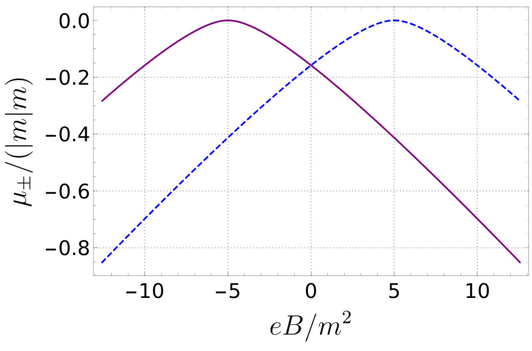 Figure 1
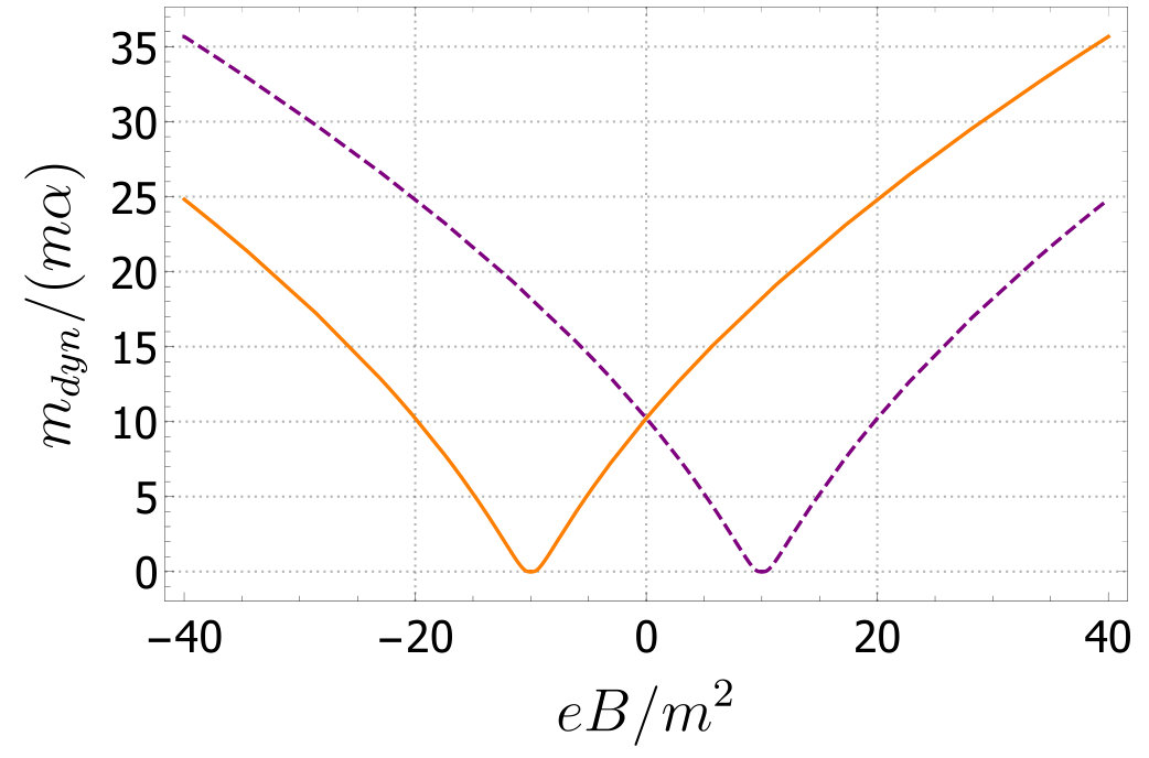 Figure 2
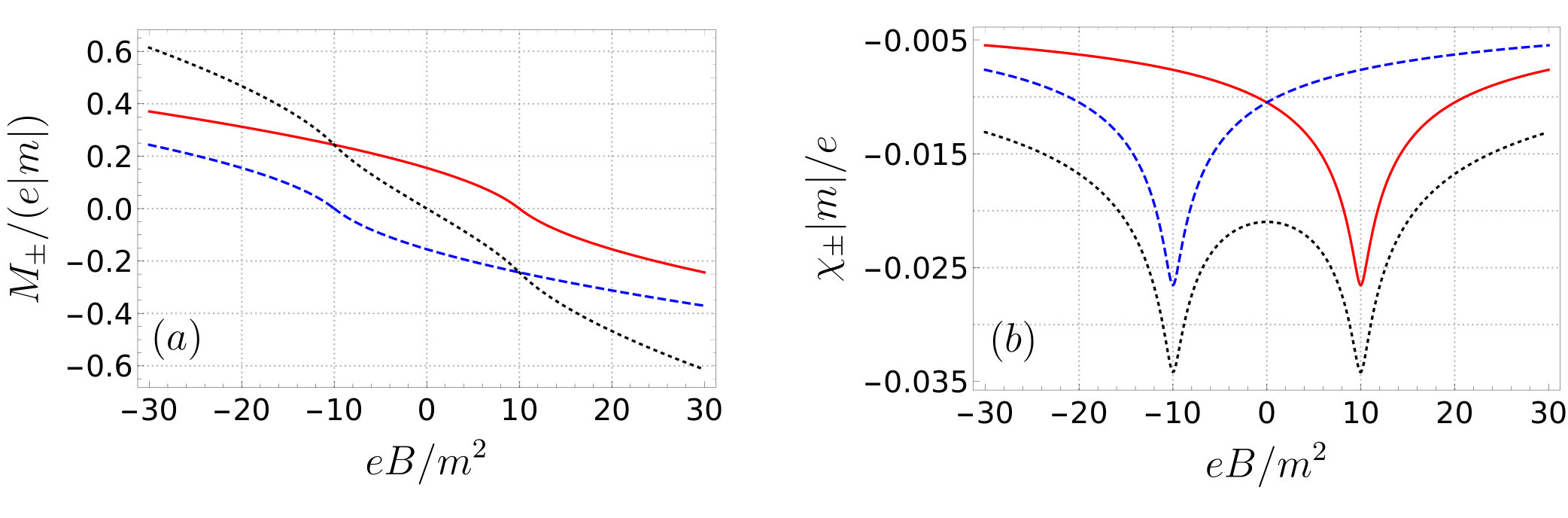 Figure 3
Peer Reviews
No public reviews on file for this paper yet. If you reviewed it on a platform where reviews are public (OpenReview, ICLR, NeurIPS, ICML), you can paste yours below so the community can read it here.
Videos
No videos yet. Explain this paper in a talk, walkthrough, or lecture? Add one.
Taxonomy
TopicsGraphene research and applications · Quantum and electron transport phenomena · Topological Materials and Phenomena
∎
\thankstext
e1e-mail: [email protected] \thankstexte2e-mail: [email protected]
11institutetext: Departamento de Física, Universidad Nacional de Colombia, Bogotá, D. C., Colombia 22institutetext: Instituto de Física, Universidade de São Paulo, 05508-090, São Paulo, SP, Brazil
Dynamical symmetry breaking, magnetization and induced charge in graphene: Interplay between magnetic and pseudomagnetic fields
J. A. Sánchez-Monroy
\thanksrefe1,addr1,addr2
C. J. Quimbay\thanksrefe2,addr1
Abstract
In this paper, we investigate the two competing effects of strains and magnetic fields in single-layer graphene to explore its impact on various phenomena of quantum field theory, such as induced charge density, magnetic catalysis, symmetry breaking, dynamical mass generation and magnetization. We show that the interplay between strains and magnetic fields produces not only a breaking of chiral symmetry, as it happens in QED2+1, but also parity and time-reversal symmetry breaking. The last two symmetry breakings are related to the dynamical generation of a Haldane mass term. We find that it is possible to modify the magnetization and the dynamical mass independently for each valley, by strain and varying the external magnetic field. Furthermore, we discover that the presence of a non-zero pseudomagnetic field, unlike the magnetic one, allows us to observe an induced “vacuum” charge and a parity anomaly in strained graphene. Finally, because the combined effect of real and pseudomagnetic fields produces an induced valley polarization, the results presented here may provide new tools to design valleytronic devices.
1 Introduction
In recent times, a number of materials for which quasiparticle excitations behave like relativistic two-dimensional fermions have appeared in condensed matter. One of the most fascinating examples of such materials is single-layer graphene, which is a material consisting of a single-layer of graphite. Graphene exhibits many interesting features, among which are the anomalous quantum Hall effect Zhang et al. (2005), a record high Young’s modulus Lee et al. (2008), ultrahigh electron mobility Bolotin et al. (2008), as well as very high thermal conductivity Faugeras et al. (2010). The band structure of single-layer graphene has two inequivalent and degenerate valleys, and , at opposite corners of the Brillouin zone. The possibility to manipulate the valley to store and carry information defines the field of “valleytronics”, in a analogous way as the role played by spin in spintronics.
One of the most exciting aspects of the physics of single-layer graphene is that several unobservable phenomena in experiments of high energy physics may be observed, such as Klein tunneling Katsnelson et al. (2006) and “Zitterbewegung” Katsnelson and Novoselov (2007). From the point of view of quantum field theory, graphene exhibits similar features with quantum electrodynamics in three dimensions (QED2+1)111Since the electrostatic potential between two electrons on a plane is the usual Coulomb potential instead of a logarithmic potential, which is distinctive of quantum electrodynamics in dimensions (QED2+1), the theory that describes graphene at low energies is known as reduced quantum electrodynamics (RQED4,3) Marino (1993); Gorbar et al. (2001); Teber (2012). In RQED4,3, the fermions are confined to a plane; nevertheless, the electromagnetic interaction between them is three-dimensional. in such a way that it is possible to explore sophisticated aspects of three-dimensional quantum field theory; for instance, magnetic catalysis, symmetry breaking, dynamical mass generation, and anomalies, among others. It is possible, in the first place, because the two valleys can be associated with two irreducible representations of the Clifford algebra in three dimensions. In the second place, because the low-energy regime quasiparticles behave like massless relativistic fermions, where the speed of light is replaced by the Fermi velocity , which is about 300 times smaller than the speed of light.
The presence of a mass gap may turn single-layer graphene from a semimetal into a semiconductor. This can be accomplished, for example, when a single-layer graphene sheet is placed on a hexagonal boron nitride substrate Giovannetti et al. (2007); Hunt et al. (2013), or deposited on a SiO2 surface Shemella and Nayak (2009). Additionally, it has been proposed that a bandgap can be induced by vacuum fluctuations Kibis et al. (2011). Significantly, a mass gap suppresses the Klein tunneling so that this fact could be useful in the design of devices based on single-layer graphene Navarro-Giraldo and Quimbay (2018).
The phenomenon known as magnetic catalysis appears when a dynamical symmetry breaking occurs in the presence of an external magnetic field, independent of its intensity Gusynin et al. (1994); Shovkovy (2013). Since in QED2+1 the mass term breaks the chiral symmetry in a reducible representation222Because the chiral symmetry cannot be defined for irreducible representations, it does not make sense to talk about chiral symmetry breaking., magnetic catalysis rise as . Dynamical symmetry breaking is a consequence of the appearance of a nonvanishing chiral condensate , which leads to the generation of a fermion dynamical mass Gusynin et al. (1994). In particular, when single-layer graphene is subjected to an external magnetic field, a nonvanishing chiral condensate ensures that there will be a dynamical chiral symmetry breaking Gusynin et al. (1994), as well as a dynamical mass equal for each valley Farakos et al. (1998); Raya and Reyes (2010).
When a sample of single-layer graphene presents strains, ripples or curvature, the dispersion relation is modified in such a way that an effective gauge vector field coupling is induced in the low energy Dirac spectrum (the so-called pseudomagnetic field Guinea et al. (2010a)). The mechanical control over the electronic structure of graphene has been explored as a potential approach to “strain engineering” Levy et al. (2010); Zhu et al. (2015). Originally, it was observed that strain produces a strong gauge field that effectively acts as a uniform pseudomagnetic field whose intensity is greater than T Guinea et al. (2010b), a pseudomagnetic field greater than T was experimentally reported later Levy et al. (2010). This pseudomagnetic field opens the door to previously inaccessible high magnetic field regimes.
In contrast to the case of a real external magnetic field, the pseudomagnetic field experienced by the particles in the valleys and have opposite signs. Hence, when a sample of strain single-layer graphene is placed in a perpendicular magnetic field, the energy levels suffer a different separation for each valley, which results in an induced valley polarization Low and Guinea (2010). The previous one is precisely the key requirement for valleytronic devices. Beyond theoretical calculations, the presence of Landau Levels in graphene has been experimentally observed in external magnetic fields Jiang et al. (2007), strain-induced pseudomagnetic fields Levy et al. (2010); Yan et al. (2012) and in the coexistence of pseudomagnetic fields and external magnetic fields Li et al. (2015). Moreover, the effects of the combination of an external magnetic field and a strain-induced pseudomagnetic field in different configurations were studied in order to construct a valley filter Zhai et al. (2010); Chaves et al. (2010); Fujita et al. (2010); Zhai et al. (2011).
In the first part of this paper, we study how an interplay between real and pseudomagnetic fields affects the symmetry breaking and the dynamical mass generation. As we will see, the presence of these two fields produces not only a breaking of chiral symmetry but also parity and time-reversal symmetry breaking. Furthermore, we will show that there will be a dynamical mass generation of two types, the usual mass () and another known as Haldane mass Haldane (1988), unlike QED2+1 where only the usual mass term is dynamically generated. As a result of this, the dynamical fermion masses will be different for each valley. In this paper, we will use a non-perturbative method based on the quantized solutions of the Dirac equation, the so-called Furry picture. The reason for using this method is to obtain nonperturbative results since the effective coupling constant in graphene is of order unity, , raising serious questions about the validity of the perturbation expansion in graphene Kolomeisky (2015). However, the latter has been a matter of controversy, since at low energy it was experimentally observed that the effective fine-structure constant approaches Reed et al. (2010).
In the second part, we investigate how the presence of real and pseudomagnetic fields affects the magnetization. In conventional metals, the magnetism receives contributions from spin (Pauli paramagnetism) and orbitals (Landau diamagnetism). In particular, the orbital magnetization of graphene in a magnetic field has shown a non-linear behavior as a function of the applied field Slizovskiy and Betouras (2012). In order to examine how the magnetization and the susceptibility behave for each valley in the presence of constant magnetic and pseudomagnetic fields, we will first obtain the one-loop effective action. The one-loop effective action without strains in dimensions had been previously calculated within the Schwinger’s proper time formalism Redlich (1984); Andersen and Haugset (1995); Dittrich and Gies (1997) and using the fermion propagator expanded over the Landau levels Ayala et al. (2010a). Taking into account that in static background fields the one-loop effective action is proportional to the vacuum energy Weinberg (1996), which can be calculated in a direct way employing the furry picture, we use this method to study the most general case. As we will show, the presence of magnetic and pseudomagnetic fields allows us to manipulate the magnetization and the susceptibility of each valley independently.
Finally, we study the parity anomaly and the induced vacuum charge in strained single-layer graphene. In quantum field theory, if a classical symmetry is not conserved at a quantum level, it is then said that the theory suffers from an anomaly. For instance, in QED2+1 if one maintains an invariant gauge regularization in all the calculations, with an odd number of fermion species, the parity symmetry is not preserved by quantum corrections, i.e. it has a parity anomaly Niemi and Semenoff (1983); Semenoff (1984); Redlich (1984). In this way, the quantum correction to the vacuum expectation value of the current can be computed to characterize the parity anomaly. As it was pointed out by Semenoff Semenoff (1984), external magnetic fields induce a current () of abnormal parity in the vacuum for each fermion species. Unfortunately, for a even number of fermion species, the total current is canceled: , and therefore the induced vacuum current is not directly observable. Therefore, it is possible to maintain the gauge and parity symmetries even at the quantum level Redlich (1984). In the literature, a number of scenarios were proposed to realize parity anomaly in dimensions. Haldane introduces a condensed matter lattice model in which parity anomaly takes place when the parameters reach critical values Haldane (1988). Obispo and Hott Obispo and Hott (2014, 2015) show that graphene coupling to an axial-vector gauge potentially exhibits parity anomaly and fermion charge fractionalization. Zhang and Qiu Zhang and Qiu (2017) show that in a graphene-like system, with a finite bare mass, a parity anomaly related -exciton can be generated by absorbing a specific photon. Alternatively, as Semenoff remarked Semenoff (1984), one could consider an “unphysical” field with abnormal parity coupled to the fermions, since for such field the total induced vacuum current should be different from zero and hence observable. As we will show, this field is physical, and it is just a pseudomagnetic field with a simple uniform field profile.
This paper is organized as follows: In section 2, we introduce the Dirac Hamiltonian and the symmetries for single-layer graphene in a finite mass gap. In section 3, we present the Furry picture for fermions in the presence of real and pseudomagnetic fields. In section 4, we compute the magnetic condensate and discuss how this characterizes the symmetry breaking and its connection with the dynamical mass of each valley. In section 5, the one-loop effective action and the magnetization are calculate for each valley. In section 6, we calculate the total induced vacuum charge density to show that graphene in the presence of a pseudomagnetic field exhibits a parity anomaly. In appendix A, we obtain the exact solution of the Dirac equation for uniform real and pseudomagnetic fields. In appendix B, we compare the calculation of fermionic condensate in the Furry picture with the method via fermion propagator and prove that the trace of the fermion propagator evaluated at equal space-time points must be understood as the expectation value of the commutator of two field operators. Finally, section 7 contains our conclusions.
2 Dirac Hamiltonian for graphene
In a vicinity of the Fermi points, the Dirac Hamiltonian in the presence of real () and pseudo () magnetic potentials reads () Herbut (2008); Kim et al. (2011)333The electric charge is multiplying the term only for dimensional reasons; strictly speaking, one could write to emphasize that it is independent of .
[TABLE]
where is a mass gap, , 444It turns out that one can identify as one component of a non-Abelian gauge field within the low-energy theory of graphene Roy (2011); Gopalakrishnan et al. (2012). The other two components of this non-Abelian gauge field are proportional to and , since they are off-diagonal in valley index mixing the two inequivalent valleys Roy (2011); Gopalakrishnan et al. (2012). In this case, the pseudo-gauge potential is . Assuming a smooth enough deformation in the graphene sheet, one can keep only the component , which does not mix the two inequivalent valleys Roy (2011). Hence, Eq. (1) captured the physics of low-energy strained graphene.. This Hamiltonian acts on the four-component “spinor”, , where the components take into account both two valleys ( and ) and the two sublattices (A and B) Katsnelson (2012), the quantum number associated with the two sublattices is usually referred to as pseudospin. If one wants to include the real spin, the spinor will have eight-components, and the Dirac Hamiltonian will be Roy (2011). For subsequent calculations, it is sufficient to consider , given that including the real spin only increases the degeneration of the Landau levels by two (). Since the difference between QED2+1 and RQED4,3 lies in the kinetic term of the gauge fields, and the magnetic field here is considered as an external field and the pseudomagnetic is a non-dynamical field. Then Eq. (1) is an appropriate description for strained graphene in the presence of an external magnetic field.
As a matter of convenience, we choose here the matrices as Charneski et al. (2009)
[TABLE]
so that , , and anticommute with , while commutes with and anticommutes with and . Note that () are block-diagonal, where each block is one of two inequivalent irreducible representations of the Clifford algebra in dimensions. For odd dimensions, there are two inequivalent irreducible representations of the Dirac matrices that we denote as and . The two inequivalent representations were chosen as and for and , respectively, where
[TABLE]
Given that there is no intervalley coupling, we can rewrite the Dirac Hamiltonian as , thus
[TABLE]
where and represent the Hamiltonian near of valley (representation ) and (representation ), respectively. acts in a two-component spinor that describes a fermion with pseudospin up and an antifermion with pseudospin down, while acts in a two-component spinor that describes a fermion with pseudospin down and an antifermion with pseudospin up. Thus, we obtain two decoupled Dirac equations in -dimensions
[TABLE]
Finally, we can write the Lagrangian density for this system as the sum of two Lagrangian densities for each valley
[TABLE]
where , which can be interpreted as a system describing two species of two-component spinors, one with mass and coupled to and the other with mass and coupled to . Hence, in the vicinity of the Fermi points, graphene monolayers constitute an ideal scenario to simulate the matter sector of QED2+1. In the following, we will neglect the corrections due to the effects of Coulomb interactions between the charge carriers. However, we point out that the model given by Eq. (1) is in good agreement with the experiments carried out in graphene in the presence of external magnetic fields Jiang et al. (2007); Novoselov and Geim (2007), pseudomagnetic fields Levy et al. (2010); Yan et al. (2012), and in the combination of magnetic and pseudomagnetic fields Li et al. (2015).
2.1 Symmetries in the irreducible and reducible representations
Irreducible representations: For irreducible representations, it is possible to define the parity (), charge conjugation (), and time-reversal () transformations as follows:
[TABLE]
Here and are unitary operators and is an anti-linear operator Peskin and Schroeder (1995), i.e. . One can check that the mass terms in the Dirac Lagrangian is not invariant under or . However, the combined transformation leaves the mass terms invariant, so is a symmetry of the Dirac Lagrangian Deser et al. (1982). Since the form three matrices and no other matrix anticommutes with them, the chiral symmetry cannot be defined for irreducible representations.
Reducible representation: For a reducible representation, let us take the four-component spinor . As it has been pointed out in Refs. Gomes et al. (1991); Charneski et al. (2009), because the free Lagrangian uses only three Dirac matrices, parity, charge conjugation and time-reversal transformations can be implemented by more than one operator
[TABLE]
where
[TABLE]
with and .
We present the transformation properties of some bilinears under , and transformations in Tab. 1 . Using these properties, one can easily prove that the massive (or massless) Dirac Lagrangian in dimensions for the reducible representation is invariant under , and , regardless of which transformation is used, i.e. the Dirac Lagrangian is invariant under and , and , and , or even a linear combination of this operator could be used, with some restrictions Gomes et al. (1991). In our Lagrangian, , there are bilinears given by , and , which are independent of . Therefore, any of the operators , and can be used to implement , and , respectively. Surprisingly, the transformation properties of , , and depends on . As a result, we find two non-equivalent realizations of parity, charge conjugation and time-reversal, which is unusual555In fact, there is an infinite number of non-equivalent realizations of , and since any linear combination of the two realizations found is an inequivalent realization.. For example, the terms and appear when a non-Abelian gauge field is introduced in graphene Roy (2011); Gopalakrishnan et al. (2012). In what follows we will be interested only in the Lagrangian density (20).
It should be noted that in the literature one can find two different transformations which are defined as time-reversal. One, , which acts as . The other, , which is the one considered here, Eq. (25), and is referred as Wigner time-reversal. The latter transformation was defined consistently with what has been done in four dimensions by Weinberg (Ch. 5. in Weinberg (1996)), and Peskin and Schroeder (Ch. 3. in Peskin and Schroeder (1995)). Moreover, the one that concerns the theorem is (for a detailed discussion, see sec. 11.6. in Schwartz (2014)).
The transformation properties of the electromagnetic potential are Deser et al. (1982)
[TABLE]
which leave the Lagrangian invariant. For pseudo-magnetic potential we should have
[TABLE]
so that the interaction in the Lagrangian is invariant.
For reducible representations, the transformation leaves invariant the kinetic term, where the generators are the generators of a global symmetry, with and the are taken as constants. The mass term breaks this global symmetry down to symmetry, whose generator are and Das (1997). However, when the mass vanishes, the quantum corrections generate a vacuum expectation value of (to be precise , see below), then, the symmetry would have broken down to .
It should be noted that besides the usual mass term , there is a mass term known as Haldane mass term Haldane (1988), which is invariant under the symmetry. However, this term breaks parity and time-reversal symmetries (see Tab. 1).
3 Furry picture
In this section we present the Furry picture based on the quantized solutions of the Dirac equation, and we generalize what has been done in Refs. Dunne and Hall (1996); Das and Hott (1996) for a Dirac equation in the presence of a real magnetic field to the case in which the Dirac equation is in the presence of real and pseudomagnetic fields. In static background gauge fields, the Dirac equation (19) can be rewritten as
[TABLE]
There are two possible solutions depending on the threshold states (). The positive-energy solutions () are
[TABLE]
where refers to the positive-energy solution in the representation and refers to the positive-energy solution in the representation . The negative-energy solutions () are
[TABLE]
where and are two functions such that
[TABLE]
Note that the threshold states and must be specified separately. When is a positive (negative) energy solution, the negative (positive) energy threshold is excluded, because of the factor Dunne and Hall (1996). For example, for the valley , or equivalently the representation , the positive-energy solutions for and are respectively
[TABLE]
where satisfies the first-order threshold equation
[TABLE]
and satisfies
[TABLE]
It turns out that if the solutions of (48) are normalizable, then the solutions of (49) are not, and vice versa Dunne and Hall (1996); Aharonov and Casher (1979). Now, in the absence of pseudo-magnetic field (), one has that . Thus, if is a positive-energy solution for the valley , then the valley only has the negative-energy solution . This leads to the well-known asymmetry in the spectrum of the states. Remarkably, this does not necessarily happen when there is a pseudo-magnetic field, since . Additionally, if the solutions of (48) are normalizable, this does not imply that the solutions of are not. Therefore, both valleys may have positive (or negative) energy states simultaneously. The Appendix (A) illustrates this point in the case of constant real and pseudomagnetic fields.
One can calculate the vacuum condensate (pairing between fermions and antifermions in the vacuum) in dimensions by expanding out the fermion field in a complete orthonormal set of the positive- and negative-energy solutions ()
[TABLE]
The solutions are labeled by two quantum numbers , in which the label refers to the eigenvalue , whilst the label distinguishes between degenerate states. In general, both and may take discrete and/or continuous values Dunne and Hall (1996). The and are the fermion annihilation operator and antifermion creation operator, respectively, which obey the anticommutation relations
[TABLE]
where , is the Kronecker delta if takes discrete values, or is the Dirac delta if it takes continuous values. Using the commutation relations (67), the vacuum expectation value can be written as
[TABLE]
i.e the fermion condensate is a sum over occupied negative-energy states. The tr is over the spinorial indices . Let us also write the condensate , which will be relevant to what follows, as
[TABLE]
i.e this condensate is a sum over occupied positive-energy states.
In the B, we compare the calculation of fermionic condensate in the Furry picture via fermion propagator. We prove that the trace of the fermion propagator evaluated at equal space-time points must be understood as the expectation value of the commutator of two field operators. Thus, the Schwinger’s choice Schwinger (1951), which is equivalent to perform the coincidence limit symmetrically on the time coordinate Dittrich and Reuter (1985), i.e.
[TABLE]
Besides, we argue that this must be the order parameter for chiral (or parity) symmetry breaking and not the fermionic condensate, as is commonly assumed in the literature.
4 Fermion condensate
Chiral symmetry breaking in ()- and ()-dimensional theories has been a subject of intense scrutiny over the past two decades Gusynin et al. (1994); Gusynin et al. (1995a, b, c); Gusynin et al. (1996, 1999); Dunne and Hall (1996); Dittrich and Gies (1997); Cea (1997); Cea and Tedesco (1998); Farakos and Mavromatos (1998); Farakos et al. (1998); Jona-Lasinio and Marchetti (1999); Cea and Tedesco (2000); Anguiano and Bashir (2005); Raya and Reyes (2010); Cea et al. (2012); Boyda et al. (2014); Ayala et al. (2006); Ferrer and de la Incera (2010); Ayala et al. (2010b); Khalilov and Mamsurov (2015). In the presence of a uniform magnetic field, the appearance of a nonvanishing chiral condensate in the limit , produce spontaneous chiral symmetry breaking Gusynin et al. (1994); Gusynin et al. (1995a, b). For example Gusynin et al. (1994); Gusynin et al. (1995c), in the Nambu-Jona-Lasinio (NJL) model, the spontaneous symmetry breaking occurs when the coupling constant exceeds some critical value, i.e. when . With an external uniform magnetic field , independent of the intensity of the magnetic field , the magnetic field is a strong catalyst of chiral symmetry breaking (see Ref. Shovkovy (2013) for review).
The exact expression for a fermion propagator in an external magnetic field in dimensions was found for the first time by Schwinger using the proper-time formalism Schwinger (1951). For dimensions, the fermion propagator was presented in the momentum representation by Gusynin et al. in Gusynin et al. (1994). In Gusynin et al. (1994); Gusynin et al. (1995a); Gusynin et al. (1996), the vacuum condensate was computed in the reducible representation (fourcomponent spinor) using the expression of the fermion propagator in the presence of an uniform magnetic field. On the other hand, Das and Hott introduced an alternative derivation of the magnetic condensate using the Furry Picture. This method has been used to calculate the magnetic vacuum condensate in dimensions de J. Anguiano-Galicia et al. (2007), at finite temperature Das and Hott (1996); Das (1997); Cea and Tedesco (1998, 2000), and as well as in the presence of parity-violating mass terms de J. Anguiano-Galicia et al. (2007). In appendix B.1, we compute the vacuum condensate in the presence of an external magnetic field for the two irreducible representations and show that these two methods are consistent if we take the definition of the propagator in equal times, as the one introduced by Schwinger in Schwinger (1951). Furthermore, we discuss why the vacuum expectation value of the commutator of two field operators is the appropriate order parameter to describe chiral (or parity) symmetry breaking.
In order to study the effect of strains, in the following we consider a sample of graphene in the presence of constant real () and pseudo () magnetic fields666We noted that the pseudomagnetic field study here is mathematically equivalent to considering a Dirac oscillator potential in -dimensions Quimbay and Strange (2013). Consequently, a constant pseudomagnetic field can be seen as a physical realization of the two-dimensional Dirac oscillator.. In this case, we choose and . The explicit solution can be found in the (A). In a similar way shown in B.1, we compute the vacuum expectation value of the commutator in the two irreducible representations for arbitrary values of , and , i.e.,
[TABLE]
with , here the sign refers to the representation (valley ), whereas refers to the representation (valley ). is the Hurwitz zeta function defined by
[TABLE]
The commutator can be rewritten in an integral representation as
[TABLE]
where we have used that
[TABLE]
which can be obtained after regularization with the integration technique Dittrich and Gies (2000). Although Eq. (4) is divergent, the divergences are already present for zero external field
[TABLE]
Therefore, by subtracting out the vacuum part, a finite result is obtained Dittrich and Gies (2000); Ayala et al. (2010b); Farakos et al. (1998)
[TABLE]
To evaluate in a simple form Eq. (109), first note that although this integral is divergent, Eq. (105) has a finite limit as if we used the analytic continuation of the Hurwitz zeta function so , which coincides with the regularization using the -integration technique Dittrich and Gies (2000). Henceforth, we will refer to as the condensates, which in terms of the analytically continue Hurwitz zeta function are given by777For numerical calculations, instead of utilizing the integral (110), the condensates can be evaluated in a much more efficient way using the Hurwitz zeta functions.
[TABLE]
One can show that there is no critical value of the fields in which the changes sign. Notably, if or , the values of the for each valley are different and when one of the two is zero, as showed in Fig. 1. Finally, let us take the limit
[TABLE]
As we will see below, this is related to a breaking of chiral, parity and time-reversal symmetries.
4.1 Dynamical mass
Dynamical mass generation in QED2+1 has been a subject of study in the past three decades Hoshino and Matsuyama (1989); Gusynin et al. (1994); Shpagin (1996); Farakos and Mavromatos (1998); Farakos et al. (1998); Raya and Reyes (2010); Khalilov (2019). As shown in Ref. Raya and Reyes (2010), the dynamical mass with a two-component fermion in a uniform magnetic field, in the so-called constant-mass approximation, is
[TABLE]
with the Euler constant, and the Lambert function. In the latter formula, it is necessary that for consistency. For weak magnetic fields, the dynamical mass has a quadratic behavior in the magnetic field, Farakos et al. (2000). Futhermore, the radiative corrections to the mass of a charged fermion when it occupies the lowest Landau level in RQED4,3 was recently computed in the one-loop approximation in Refs. Khalilov (2019); Machet (2018). Its associated equation reads
[TABLE]
with and where erfc and are the complementary error function and upper incomplete gamma function, respectively. Significantly, the dynamical mass does not vanish even at the limit of zero bare mass () Machet (2018); Khalilov (2019)
[TABLE]
In graphene, while the photon propagates in spatial dimensions, the fermions are localized on spatial dimensions, because of this, RQED4,3 is an appropriate model to describe the low-energy physics for this system. Nevertheless, as mentioned above, the coupling constant is large, hence, this perturbative result is not necessarily accurate Kolomeisky (2015); Khalilov (2019). In the following, because of the lack of a better estimate, we use this result to determine the dynamical mass in graphene.
In general, the dynamical mass should be given by , where is a general function. It is straightforward to extend this result to include the pseudomagnetic field. Hence, the dynamical mass would read as and we thus obtain
[TABLE]
with . According to these findings, the dynamical fermion mass is different for each valley, for and for (see Fig. 2). This is not surprising since the condensates, and , are different if a pseudomagnetic field is included. Furthermore, it is possible to construct a Lagrangian that describes two species of fermions, each with different mass, introducing the usual mass term () and a Haldane mass term ()
[TABLE]
In this case, the two masses will be and is taken as a four-component spinor. This result implies that the interplay between the real and pseudomagnetic fields allows us to dynamically generate these two terms. With the help of Eq. (112), one can realize that
[TABLE]
while in the limit , we have
[TABLE]
Therefore, the usual mass term is always generated independently of and , whereas the Haldane mass term is only generated if and simultaneously. Note that when (or ), one of the condensates is zero and the dynamical mass of this valley will be independent of and .
Finally, it is important to realize that for zero pseudomagnetic field, the mass term in irreducible representations breaks parity and time-reversal symmetries, while in a reducible representation chirality is broken. Thus, for irreducible representations, the condensate () is the order parameter of the dynamical parity and there is a time-reversal symmetry breaking. In contrast, dynamical symmetry breaking occurs in reducible representations. In reducible representations, however, non-zero magnetic and pseudo magnetic fields produce a dynamical symmetry breaking, not only of the chiral symmetry but also of the parity and time-reversal symmetries888In Ref. Herbut (2008), it had been suggested that the flux of the non-Abelian pseudomagnetic field catalyzes the time-reversal symmetry breaking.. The reason for this is that by including pseudomagnetic field, the dynamical mass is different for each valley since a Haldane mass term (which breaks parity and time reversal) is generated999The Haldane mass term, for example, can also be dynamically generated in graphene at sufficiently large strength of the long-range Coulomb interaction González (2013)..
5 One-loop effective action and magnetization
In this section we compute the effective action and the magnetization in the presence of uniform real and pseudomagnetic fields. We consider the fermionic part of the generating functional for each valley
[TABLE]
Then, we introduce the one-loop effective Lagrangian via . In the presence of a static background field, the one-loop effective action is proportional to the vacuum energy (Ch. 16. in Weinberg (1996)). The vacuum energy of the Dirac energy field can be computed using the formula Plunien et al. (1986)
[TABLE]
which depends upon the zero-point energies of both positive- and negative-energy states101010Provided that for each eigenvalue , there is an eigenvalue , then the two sums in Eq. (121) reduces to the sum over the Dirac sea
This equation is always satisfied by a charge conjugation invariant background; however, this is not our case. The use of this equation in a magnetic field background has led to erroneous conclusions in Ref. Cea (1985); Cea and Tedesco (2000).. In our case, it is straightforward to obtain the density vacuum energy for each valley
[TABLE]
where we have used that the Landau degeneracy per unit area is . In order to calculate the purely magnetic field effect, we need to subtract the zero-field part. Thus, the one-loop effective Lagrangian density is111111This approach is equivalent to compute an infinite series of one–loop diagrams with the insertion of one, two, …external lines (see for instance Ref. Dittrich and Reuter (1985)).
[TABLE]
Using Eq. (108), we can rewritten the one-loop effective Lagrangian in an integral representation such as
[TABLE]
For , the result is in agreement with what was found in Ref. Redlich (1984); Andersen and Haugset (1995); Dittrich and Gies (1997); Ayala et al. (2010a). In particular, when , we arrive to
[TABLE]
Here is the Riemann-zeta function. One can compute the orbital magnetization for each valley () employing the one-loop effective Lagrangian, namely . A straightforward calculation gives
[TABLE]
which can also be written as
[TABLE]
Therefore, the orbital magnetization displays nonlinear behavior in the magnetic and pseudomagnetic fields (see Fig. 3a). For , the result is in agreement with Refs. Andersen and Haugset (1995); Ayala et al. (2010a); Slizovskiy and Betouras (2012) and in the limit the magnetization is
[TABLE]
for each valley121212It should be noted that Eq. (128) also corresponds to the dominant term in the strong field expansion.. Notably, the value and sign of magnetization are different for each valley. Thus, they can be modified by the strains or varying the applied magnetic field. In particular, the magnetization of one valley could be zero while the other does not, as it can be seen in Fig. 3a.
Having calculated , one can compute the magnetic susceptibility for each valley in the presence of magnetic and pseudomagnetic fields, which is simply given by , thus
[TABLE]
In the presence of magnetic and pseudomagnetic fields, the total susceptibility has two minimums, see Fig. 3b, which is a distinctive feature compared with the case Slizovskiy and Betouras (2012). Finally, in the limit the susceptibility is
[TABLE]
which is divergent when . Since is finite, it can be concluded that the mass acts as a regulator.
6 Induced charge density
In this section, we derive an expression for the induced charge density in the presence of uniform real and pseudomagnetic fields. We first noticed, that as in the case of the fermionic condensate, the formula also deserves to be revised. The current must be understood as
[TABLE]
which is the correct definition of the current operator, where it has been subtracted an infinite charge of the vacuum state Dittrich and Reuter (1985). In an analogous way to what was done before, we can find that in the Furry picture the vacuum expectation value of the current operator is
[TABLE]
For constant real and pseudomagnetic fields, using the orthogonality of Hermite polynomials, one can show that
[TABLE]
i.e the induced current vanishes. A nonvanishing vacuum current would arise in the presence of an external electric field Andersen and Haugset (1995). On the other hand, the induced charge density is given by
[TABLE]
Curiously, in contrast to , the induced charge density only receives contributions from the lowest Landau level (LLL), even if . An alternative technique to compute the charge density is through spectral function. It can be shown that the induced charge is Reuter and Dittrich (1986); Dittrich and Reuter (1986)
[TABLE]
where
[TABLE]
is the invariant of Atiyah, Patodi, and Singer. Using the Landau degeneracy per unit area and noting that except for the LLL, for each eigenvalue there is an eigenvalue , then we obtain Eq. (151) as we should. Therefore, the total induced charge density is
[TABLE]
which is observable (and measurable) when taking a nonzero pseudomagnetic field. This is remarkable since this is not possible in the case of a pure magnetic field Semenoff (1984). Eq. (154) shows that in the presence of pseudomagnetic fields, the system has a parity anomaly, even with two fermionic species. Eqs. (150) and (151) are related with the Chern-Simons relation, which in the case of zero pseudomagnetic field reads Semenoff (1984)
[TABLE]
It is clear from this equation equation that when the two representations are present, the vacuum expectation value of the total current is always zero.
7 Conclusions
In summary, we have examined the Dirac Hamiltonian in dimensions and found an infinite number of non-equivalent realizations of parity, charge conjugation, and time-reversal transformations for the reducible representation. We have then explored how the interplay between real and pseudomagnetic fields affects some aspects of the three-dimensional quantum field theory. For the case of uniform magnetic and pseudomagnetic fields, by employing a non-perturbative approach we have found that: (i) The condensate is the appropriate order parameter for studying the breaking of chiral, parity and time-reversal symmetries. (ii) One can control the magnetization, susceptibility, and the dynamical mass independently for each valley by straining and varying the applied magnetic field. (iii) The dynamical mass generated is due to two terms, the usual mass term () and a Haldane mass term (), being the latter, for the case in which the two fields are simultaneously different from zero, the one that breaks parity and time-reversal symmetries. (iv) For non-zero pseudomagnetic field, the total induced “vacuum” charge density is not null. This last result implies that strained single-layer graphene exhibits a parity anomaly. Therefore, strained graphene in the presence of an external magnetic field has distinctive features compared with QED2+1, which lacks the aforementioned consequences (i)-(iv). Finally, it would be interesting to extend our calculations to include the effect of Coulomb interactions on the magnetic catalysis, symmetry breaking, dynamical mass generation, etc. See, for instance, the study of the magnetic catalysis in unstrained graphene in the weak-coupling limit Semenoff and Zhou (2011).
Acknowledgements.
J. A. Sánchez is grateful to F. T. Brandt, C. M. Acosta and J. S. Cortés for useful comments.
Appendix A Exact solutions of the Dirac equation in the presence of uniform real and pseudomagnetic fields
In the presence of a constant real () and pseudo () magnetic fields, one can choose the real potential and the pseudo-potential as and , respectively. For the valley and with , it is straightforward to find the spectrum and the solutions of Eq. (19). However, we need to find them independently for the cases and . For the first case , the spectrum and solutions are given by
[TABLE]
[TABLE]
[TABLE]
where
[TABLE]
[TABLE]
with and . Note that the lowest Landau level (LLL) describes particle (fermion) states with energy . In order to find the solutions for the case , one can use the charge-conjugate operator, Eq. (23), Abouelsaood (1985), so, the solutions are given by
[TABLE]
[TABLE]
Now the LLL describes hole (antifermion) states.
One can find the solution for the valley noting that the change of representation is equivalent to change and in the solutions (157), (158), (161) and (162). For the point , the LLL describes a hole (antifermion) state for and a particle (fermion) state for . Hence, we can have a fermion (antifermion) state in the LLL simultaneously to and if the condition () is satisfied.
Appendix B Magnetic condensate
In this Appendix, we will compare the calculation of fermionic condensate in the Furry picture with the method via fermion propagator. We then demonstrate that the method via the fermion propagator does not calculate the vacuum expectation value of the product of two field operators (magnetic condensate), but rather a vacuum expectation value of the commutator of two field operators. Finally, we show that the commutator is the order parameter is for chiral (or parity) symmetry breaking, instead of the magnetic condensate, as it is often asserted in the literature.
B.1 Magnetic condensate via furry picture
Let us consider the fermionic condensate via the Furry picture in a constant background magnetic field. The explicit solution can be found in the Appendix (A), taking . Inserting Eq. (158) into Eq. (85), we obtain that for the irreducible representation (valley ), for and , the fermion condensate is
[TABLE]
with and where we used that
[TABLE]
and that for all the terms are zero. Now, for , inserting Eq. (162) into Eq. (85) yields
[TABLE]
It is clear now that contribute to the condensate. In a similar way, the condensates in the irreducible representation (valley ) are
[TABLE]
for and , respectively. In the fermion condensates, the term is in general divergent. However, the results are understood by means of an appropriate analytic continuation.
Eqs. (163) and (168) are in agreement with what was found in Ref. Cea and Tedesco (2000). When , one just need to exchange results in Eq. (163) with the one of Eq. (167), and Eq. (168) with Eq. (169). In the limit , for massless fermions, the fermionic condensates are
[TABLE]
and
[TABLE]
Notably, only if the LLL has negative energy states there is a non-vanished magnetic condensate. The condensate in the reducible representation is simply the sum of the irreducible representations
[TABLE]
which is in agreement with the results of Refs. Dunne and Hall (1996); Das and Hott (1996); Das (1997); Farakos et al. (1998); de J. Anguiano-Galicia et al. (2007); Cea and Tedesco (2000).
B.2 Magnetic condensate via the fermion propagator
Now we consider the usual way to calculate the vacuum condensate using the fermion propagator Gusynin et al. (1994)
[TABLE]
where is the time-ordering operator
[TABLE]
with the Heaviside step function. In the presence of a magnetic field, can be calculated by using the Schwinger (proper time) approach Schwinger (1951)
[TABLE]
where the integral is calculated along the straight line, and the Fourier transform of (in Euclidean space) is ()
[TABLE]
with and the () identity matrix and the () -matrices in the reducible (irreducible) representations. The magnetic condensate has been calculated as Gusynin et al. (1994); Gusynin et al. (1995a); Gusynin et al. (1996)
[TABLE]
where the superscript emphasizes that the condensate is computed via the propagator. For the reducible representations, in the limit , the condensate reads Gusynin et al. (1994)
[TABLE]
which is in agreement with Eq. (176). However, for the irreducible representations the magnetic condensate is
[TABLE]
which is the same for both representations, but it differs from what was obtained previously in Eqs. (172) and (175). To explain why the condensates are different, let us critically review the calculation through propagator131313 Using the so-called Ritus eigenfunctions method, it has recently been found Eq. (183) Raya and Reyes (2010), however, this method also uses the propagator to calculate the condensate.. If one part of the definition of the propagator Eqs. (177) and (178), it is clear that depends on how one takes the limit, namely
[TABLE]
Using Eq. (103) one can show that, in the limit , the fermion condensates for the irreducible representations are
[TABLE]
and
[TABLE]
for the reducible representation. It is clear that for irreducible representations neither nor coincide with . The calculation of the condensate in Refs. Gusynin et al. (1994); Gusynin et al. (1995a) was actually calculated by taking . This will formally lead to calculate the propagator in , which depends on . In the literature there is not a consensus of what should be the value of . For instance, can be , [math] or (page 24 in Zee (2010)). However, the only consistent value with Eqs. (172), (175), (176), (188), (191) and (192) is the value of , since
[TABLE]
so,
[TABLE]
which gives us the correct value for all condensates. In fact this last choice was the Schwinger’s choice: “the average of the forms obtained by letting approach from the future, and from the past” Schwinger (1951). Therefore, the Heaviside step function in the fermion propagator should be understood as
[TABLE]
In summary, . We believe that this has not been noticed before since, in particular, when the condensate is computed in dimensions in a reducible representation, the two values match, which as we showed is just a coincidence141414One can show that in dimensions the two values also match, see Ref. Gusynin et al. (1995c) for the calculation via fermion propagator and reference de J. Anguiano-Galicia et al. (2007) for the calculation in the Furry picture..
B.3 Order parameter
It is widely claimed in the literature that in the reducible representations the fermion condensate is the order parameter of dynamical chiral symmetry breaking Gusynin et al. (1994); Gusynin et al. (1995a, b); Dunne and Hall (1996); Das and Hott (1996). However, as we have just showed, a part of the literature calculates and another part calculates as the order parameter, always assuming that is being calculated. Thus, we may ask what is the order parameter for chiral (or parity) symmetry breaking. Since in reducible representations the two values match, we will use the irreducible representations to solve this puzzle.
Although in irreducible representations we have not a chiral symmetry, as we mentioned above, the mass term breaks parity and time-reversal symmetry. If the fermion condensate is the order parameter of dynamical parity and time-reversal symmetry breaking, Eqs. (172) and (175) would lead us to conclude that these broken symmetries depend on the magnetic field orientation. Moreover, since the fermionic condensate is zero for () in the representation () there would not be a dynamical symmetry breaking in this case and therefore would not have a magnetically induced mass. However, if the order parameter is the commutator, which is independent of the orientation of the magnetic field and the representation, we would obtain a magnetically induced mass for .
In QED2+1 and RQED4,3 the dynamical mass generation has already been investigated Hoshino and Matsuyama (1989); Gusynin et al. (1994); Shpagin (1996); Farakos and Mavromatos (1998); Farakos et al. (1998); Raya and Reyes (2010); Khalilov (2019). In particular, the dynamical mass generation with a two-component fermion was examined in Hoshino and Matsuyama (1989); Raya and Reyes (2010); Khalilov (2019). From the results of these works, it can be concluded that there is no evidence that the dynamical mass depends on the orientation of the magnetic field. Moreover, under some assumptions, an explicit formula was found for the dynamical mass when it is much smaller than the magnetic field Raya and Reyes (2010). One can show that the dynamic mass found is independent of the orientation and the representation of the -matrices. Therefore, the order parameter for parity (or chiral) symmetry breaking is not the vacuum expectation value of the product of two field operators (magnetic condensate), but rather a vacuum expectation value of the commutator of two field operators. The latter is equivalent to the trace of the fermion propagator evaluated at equal space-time points.
The reference list from the paper itself. Each links out to its DOI / PubMed record.
- 1Zhang et al. (2005) Y. Zhang, Y.-W. Tan, H. L. Stormer, and P. Kim, Nature 438 , 201 (2005).
- 2Lee et al. (2008) C. Lee, X. Wei, J. W. Kysar, and J. Hone, Science 321 , 385 (2008).
- 3Bolotin et al. (2008) K. Bolotin, K. Sikes, Z. Jiang, M. Klima, G. Fudenberg, J. Hone, P. Kim, and H. Stormer, Solid State Communications 146 , 351 (2008).
- 4Faugeras et al. (2010) C. Faugeras, B. Faugeras, M. Orlita, M. Potemski, R. R. Nair, and A. Geim, ACS nano 4 , 1889 (2010).
- 5Katsnelson et al. (2006) M. Katsnelson, K. Novoselov, and A. Geim, Nature physics 2 , 620 (2006).
- 6Katsnelson and Novoselov (2007) M. Katsnelson and K. Novoselov, Solid State Communications 143 , 3 (2007).
- 7Marino (1993) E. Marino, Nucl. Phys. B 408 , 551 (1993).
- 8Gorbar et al. (2001) E. V. Gorbar, V. P. Gusynin, and V. A. Miransky, Phys. Rev. D 64 , 105028 (2001).