Manifolds pinned by a high-dimensional random landscape: Hessian at the global energy minimum
Yan V. Fyodorov, Pierre Le Doussal

TL;DR
This paper analyzes the spectral properties of the Hessian matrix at the energy minimum of a high-dimensional elastic manifold in a random landscape, revealing phase transitions and spectral gaps related to the confinement strength and replica symmetry breaking.
Contribution
It extends previous zero-dimensional results to finite internal dimensions, deriving the spectral density equations and analyzing the transition between replica-symmetric and RSB phases in high-dimensional systems.
Findings
For confinement curvature above a critical value, the Hessian spectrum is gapped.
The spectral gap vanishes quadratically at the transition point.
In the RSB phase, the spectrum can be gapless or have a zero edge depending on the RSB type.
Abstract
We consider an elastic manifold of internal dimension and length pinned in a dimensional random potential and confined by an additional parabolic potential of curvature . We are interested in the mean spectral density of the Hessian matrix at the absolute minimum of the total energy. We use the replica approach to derive the system of equations for for a fixed in the limit extending results of our previous work. A particular attention is devoted to analyzing the limit of extended lattice systems by letting . In all cases we show that for a confinement curvature exceeding a critical value , the so-called "Larkin mass", the system is replica-symmetric and the Hessian spectrum is always gapped (from zero). The gap vanishes quadratically at . For the replica…
Click any figure to enlarge with its caption.
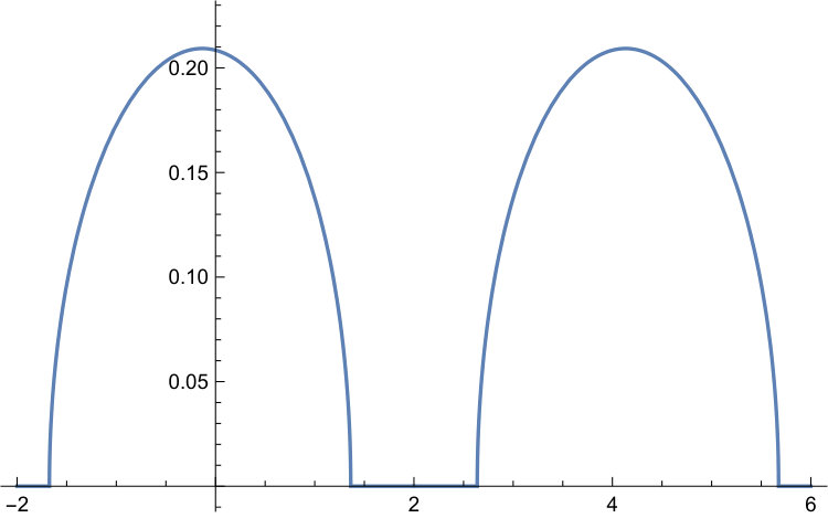 Figure 1
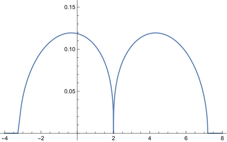 Figure 2
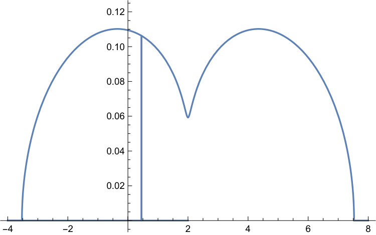 Figure 3
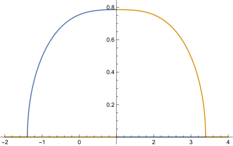 Figure 4
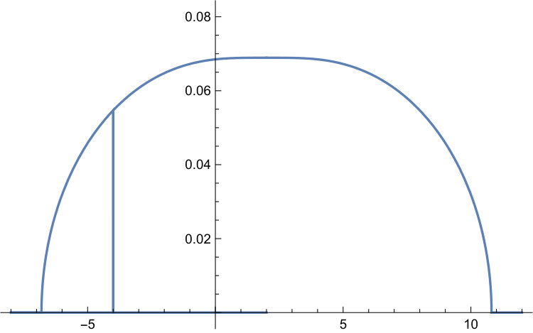 Figure 5
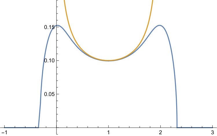 Figure 6
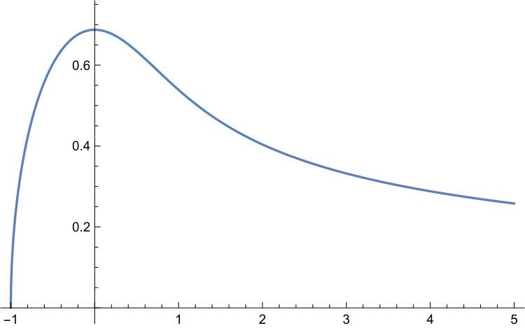 Figure 7
Peer Reviews
No public reviews on file for this paper yet. If you reviewed it on a platform where reviews are public (OpenReview, ICLR, NeurIPS, ICML), you can paste yours below so the community can read it here.
Videos
No videos yet. Explain this paper in a talk, walkthrough, or lecture? Add one.
Manifolds pinned by a high-dimensional random landscape: Hessian at the global energy minimum.
Yan V. Fyodorov
King’s College London, Department of Mathematics, London WC2R 2LS, United Kingdom
Pierre Le Doussal
Laboratoire de Physique de l’Ecole Normale Supérieure, PSL University, CNRS, Sorbonne Universités, 24 rue Lhomond, 75231 Paris, France
Abstract
We consider an elastic manifold of internal dimension and length pinned in a dimensional random potential and confined by an additional parabolic potential of curvature . We are interested in the mean spectral density of the Hessian matrix at the absolute minimum of the total energy. We use the replica approach to derive the system of equations for for a fixed in the limit extending results of our previous work [11]. A particular attention is devoted to analyzing the limit of extended lattice systems by letting . In all cases we show that for a confinement curvature exceeding a critical value , the so-called ”Larkin mass”, the system is replica-symmetric and the Hessian spectrum is always gapped (from zero). The gap vanishes quadratically at . For the replica symmetry breaking (RSB) occurs and the Hessian spectrum is either gapped or extends down to zero, depending on whether RSB is 1-step or full. In the 1-RSB case the gap vanishes in all as near the transition. In the full RSB case the gap is identically zero. A set of specific landscapes realize the so-called ”marginal cases” in which share both feature of the 1-step and the full RSB solution, and exhibit some scale invariance. We also obtain the average Green function associated to the Hessian and find that at the edge of the spectrum it decays exponentially in the distance within the internal space of the manifold with a length scale equal in all cases to the Larkin length introduced in the theory of pinning.
1 Introduction
1.1 The random manifold model and some known results
Numerous physical systems can be modeled by a collection of points or particles coupled by an elastic energy, usually called an elastic manifold, submitted to a random potential (see [1, 2, 3] for reviews). They are often called ”disordered elastic systems” and generically exhibit pinning in their statics and depinning transitions and avalanches in their driven dynamics [4, 9, 5, 6, 7, 8]. Their energy landscape is complex leading to glassy behavior.
The manifold is usually parameterized by a -component real displacement field , where belongs to an internal space . can be either a finite collection of points, such as a subset of an internal space of dimension , , for discrete models, or in a continous setting. The case corresponds to a line in dimensions and for was studied in the present context in [10]. The case usually refers below to being a single point, previously studied in [11] in the large limit, and the present study can be seen as its generalization to a manifold. There are two terms in the total energy. First the points in are coupled via an elastic energy, which is a quadratic form in the fields . We also include in this quadratic term a parabolic confining potential of curvature . The absolute minimum of this first term is thus the flat, undisturbed, configuration . The second term is the quenched disorder, modeled by a random potential energy which couples directly to . We thus consider the following model of an elastic manifold in a random potential given by its energy functional
[TABLE]
where here , is an appropriate identity operator, and the matrix is required to be positive definite. Here can be chosen as the discrete Laplacian in the hypercube with periodic boundary conditions. In that case its eigenmodes are plane waves and we denote its eigenvalues, i.e. in , with , . For general similar formula holds and must be positive, . All formula below extend immediately to more general functions , e.g. to more general elasticity (such as long range elasticity). They also extend to cases where is a quadratic form defined on any graph . Finally, they also extend to the limit of the continuum manifold model, e.g. with the standard Laplacian whose spectrum is given by . We thus use the notation so our main formula are valid both for discrete and continuum (in the continuum ). We see from (1) that acts as a “mass” which, for the continuum model, leads to reducing the fluctuations beyond the scale .
Here we will consider to be a mean-zero Gaussian-distributed random potential in with a rotational and translational invariant covariance (also called the correlator in the physical context) such that potential values are uncorrelated for different points in the internal space, but correlated for different displacements: 111We follow here the same notations as in [12, 13, 14, 15]. Note the factor of difference with the definition of in [11]. Noting the similar function there, we have . defined below is the same object in both papers.
[TABLE]
In Eq.(2) and henceforth the notation stands for the quantities averaged over the random potential.
The equilibrium statics of this model has been much studied. From the competition between the elastic and the disorder energy, the minimal energy configuration (ground state) is non trivial and exhibits interesting statistically self-affine properties characterized by a roughness exponent: . The sample to sample fluctuations of the ground state energy (and, at finite temperature, of the free energy) grow with the scale as , with as a consequence of the symmetries of the model (1)-(2). In addition the manifold is pinned, i.e. its macroscopic response to an external force is non-linear. The early (and partly phenomenological) theory of pinning is due to Larkin and Ovchinnikov (see [1] for a review). Below the so-called Larkin length scale , with for weak disorder (small ) the deformations are elastic, the response is linear, deformations can be calculated from perturbation theory, leading to the roughness exponent . Above metastability sets in, the response to perturbations involves jumps (shocks), with non-trivial roughness of minimal energy configurations. Describing that regime has been a challenge, and progress was later achieved using the bag of tools of the statistical mechanics of disordered systems, most notably replica methods. Exact results have been obtained, but in only a few analytically tractable cases. The first of such cases are mean field type models, notably the model (1) in the limit . Saddle point equations in replica space [17, 16, 15, 14] lead to solutions exhibiting replica symmetry breaking (RSB) for , which describe the glass phase where the manifold is pinned. The critical mass corresponds to the Larkin scale and the glass phase appears at scales exceeding . A second set of results were obtained using the functional renormalization group [2, 18, 20, 19] and are valid in an expansion around (for any ). While the resulting physical picture is somewhat different, these could be reconciled [14, 15]. Note also that the Larkin picture was fully confirmed by these studies. Finally, for the problem can be mapped to stirred Burgers and Kardar-Parisi-Zhang growth (see Ref. [21] for review of earlier works). For , a number of exact results were obtained recently from an emerging integrability structure of the theory, both in physics and mathematics. Besides proving the exact roughness and free energy fluctuation exponent, , it was shown, e.g., that the probability density of the free energy for a long polymer converges to the famous Tracy-Widom distribution both at zero temperature [22], and at finite temperature in the continuum [23, 24, 25, 26, 27]. Finally, note that the model (1)-(2) also arises in the study of the decaying Burgers equation with a random initial conditions in dimension , which exhibits interesting transitions and regimes, see e.g. for [28] and for large [29].
1.2 Motivation and goals of the paper
While these results predict large scale properties of the low energy configurations, little is known about the detailed statistical structure of the complex energy landscape of pinned manifolds. This relates to the broad effort of understanding the statistical structure of stationary points (minima, maxima and saddles) of random landscapes which is of steady interest in theoretical physics [30, 31, 32, 33, 34, 35, 36, 37, 38, 39], with recent applications to statistical physics [34, 35, 36, 38, 39, 40, 10, 41], neural networks and complex dynamics [42, 43, 44, 45, 46], string theory [47, 48] and cosmology [49, 50]. It is also of active current interest in pure and applied mathematics [51, 53, 54, 55, 52, 56, 57, 58, 59, 60], For the model (1)-(2) in the simplest case ( is a single point), the mean number of stationary points and of minima of the energy function was investigated in the limit of large in [35, 38, 39], see also [37, 52, 50]. It was found that a sharp transition occurs from a ’simple’ landscape for (the same as given by the onset of RSB, see above), with typically only a single stationary point (the minimum) to a complex (’glassy’) landscapes for with exponentially many stationary points. Similar transitions were found in related systems upon applying various external perturbations [40, 44, 41] in particular in the mean number of stationary points which was also studied recently for the case of an elastic string in dimension [10]. Relations with Anderson localization was discussed there in this context.
An important quantity which characterizes the stability of local equilibria, and is crucial both for equilibrium and slowly driven dynamics, is the Hessian matrix. In particular, the question of whether the spectrum of the Hessian at low lying local minima is gapped (away from zero) or not, the behavior of its mean density of eigenvalues near zero, and the nature of the associated low lying modes, has been identified as a crucial feature to describe classical [61, 62, 63] and quantum glasses [64, 65, 66, 67, 68]. Clearly, a ’gapless’ spectrum reflects the existence of very ’flat’ directions in configuration space along which moving away from the local minimum incurs very little ’cost’. This flatness, also known as a ’marginal stability’, is ubiquitous in various types of glasses [62, 63] and appears naturally in models exhibiting a hierarchical structure of the energy landscapes [69, 70]. The Hessian matrix was studied recently numerically in the context of the depinning of an elastic line in a one dimension random potential, , in an effort to identify the ”soft modes” which trigger the avalanches. It was found that in the stationary state reached upon quasi-static driving, the low-lying modes of the Hessian are localized, with a localization length directly related to the Larkin pinning length [71]. Although studying the Hessian at equilibrium, and specifically at the global minimum would be also very interesting, it is analytically challenging for or small.
Recently, by combining methods of random matrix theory with methods of statistical mechanics of disordered systems, we were able to study the Hessian at the absolute minimum for the particle model () in the limit of large [11]. The main goal of the present paper is to extend this study to the pinned elastic manifold. Hence we will study the Hessian matrix
[TABLE]
in particular its density of eigenvalues normalized as . An important feature of such matrix is its (block-)band structure visualized below:
(\mu+2t){\bf 1}_{N}$$-t{\bf 1}_{N}$$-t{\bf 1}_{N}$$+{\bf W}^{(1)}$$-t{\bf 1}_{N}$$(\mu+2t){\bf 1}_{N}$$+{\bf W}^{(2)}$$-t{\bf 1}_{N}$$-t{\bf 1}_{N}$$-t{\bf 1}_{N}$$-t{\bf 1}_{N}$$(\mu+2t){\bf 1}_{N}$$+{\bf W}^{(L)}$$-t{\bf 1}_{N}$$\mbox{\sf Structure of the}\,\,(NL\times NL)\,\,\mbox{\sf Hessian matrix }K in 1d discrete lattice model with internal sites and periodic boundary conditions.Only non-zero blocks are indicated.
where for we have introduced random matrices with entries {\bf W}^{(r)}_{ij}=\frac{\partial^{2}}{\partial u_{i}\partial u_{j}}V({\bf u}(x),x)\big{|}_{x=x_{r}}.
Our main focus here is the problem where the Hessian is chosen at the global minimal energy configuration . At the same time it is worth noting another interesting problem, where the Hessian is not conditioned by the global energy minimum, but instead chosen at a generic point in configuration space, i.e. at an arbitrary fixed . It is easy to see from (3) and from the statistical translational invariance of the correlator in (2) that the Hessian is then statistically independent of the choice of , i.e. we may as well chose it at . The covariance structure of the random potential (2) implies, after a simple differentiation that entries of the matrices are mean-zero Gaussian-distributed, independent for different and have the following covariance structure:
[TABLE]
The matrices of such block-band type, with in diagonal blocks replaced with GOE matrices with i.i.d. entries, were introduced by Wegner[72] in his famous studies of the Anderson localization, and are now known by the general name of Wigner orbital models. Various instances of the models kept attracting attention in Theoretical and Mathematical Physics literature over the years, see e.g. recent paper [73] and references therein. In particular, the mean eigenvalue density for such type of models as is known to be determined by the deformed semicircle equation rigorously derived in [74]. That equation naturally generalizes the so-called Pastur equation of random matrix theory [75]. We will see below that the difference between GOE covariance and our choice (4) is immaterial for the calculation of the mean eigenvalue density which will be found to satisfy exactly the same deformed semicircle equation. Moreover, when we condition the Hessian by being at the global energy minimum the equation retains its validity, albeit with the renormalized curvature parameter , which should be determined by a separate minimization procedure. The replacement is crucial in determining the global position of the support of the density of states, i.e. the position of the edge(s) and the value of the gap, for the Hessian at the global energy minimum, but the general form of the density can be already determined without that knowledge by studying the above mentioned equation.
An analysis of the density profile following from that equation hence comes naturally in our problem as by-product of its solution. Surprisingly, we were not able to trace it in the literature for the most interesting case of infinite system of size . As it may have a separate interest and is quite instructive, we are going to fill in that gap in the present paper and provide such an analysis for .
In the case of a continuous manifold the Hessian matrix becomes a matrix-valued differential operator acting in the space of component vectors where, e.g. , by the following rule:
[TABLE]
with appropriate boundary conditions (e.g. periodic, or Dirichlet).
Without conditioning by global minimum the covariance structure of is a natural analogue of (4):
[TABLE]
In particular, for the operator can be visualized in the following form of an matrix 222Note that in such a case the spectral density in the infinite-volume limit can not be normalized. E.g. recall the density for the disorder-free model with given by .:
[TABLE]
Models of such type are sometimes called the matrix Anderson models, and are essentially continuous versions of Wegner orbital models. Again, we will show below that the associated ’deformed semicircle’ equation for the mean eigenvalue density of such problem can be solved as long as and yields an explicit form of the density profile.
2 Summary of the main results
In this paper our main object of interest is the disorder-averaged resolvent (Green’s function) of the Hessian, calculated at the absolute minimum of the total energy:
[TABLE]
as well as its limit at coinciding points , which relates to the mean spectral density of the Hessian as
[TABLE]
Employing the replica trick, we first show that for (the limit being taken for a fixed value of ) the average Green’s function is given by
[TABLE]
where the value of the parameter is determined by the following self-consistent ’deformed semicircle’ equation for the diagonal part
[TABLE]
which is essentially of the same form as one for the orbital model with lattice Laplacian [74].
The only quantity which contains all the information about the optimization leading to the ground state is the parameter . Below will be calculated in the various cases (replica-symmetric, 1RSB and FRSB) in the framework of the replica theory. We recall that the notation applies both to the discrete models and the continuum limit . These equations are quite general and apply to basically arbitrary graph Laplacian matrices (even not translationally invariant ones, provided the formula are are generalized by replacing , i.e. the trace in internal space of the inverse matrix).
2.1 Spectral Density of the Hessian at a generic point
As has been already mentioned, with setting the above expressions (10, 11) provides the mean resolvent and the mean spectral density for the manifold Hessian around a generic point of the disordered landscape. Such object is interesting by itself and we study the shapes of the spectral density in detail for several examples. Its generic feature is the square-root singularity at the spectral edges, which is thus a universal characteristics of the mean-field type spectral densities for disordered elastic systems of any dimension . The shape as a whole is not universal and essentially depends on the dimension and the type of the Laplacian matrix (discrete or continuous).
As relatively few explicit formulas are available in the literature for eigenvalue densities of disordered matrices and operators beyond Wigner semicircular, Marchenko-Pastur and 1D chains ( see the book [76] for those and further examples) we want to emphasize that in our model it turns out to be possible to find explicitly the spectral density for the 1D matrix Anderson model (7), of infinite length and the Laplacian spectrum :
[TABLE]
where
[TABLE]
We have plotted in the Fig. 1 the parameter free scaling function . The spectral edge is given in this case by . The function reaches its maximum at and then decays at as . The latter regime corresponds to the spectral density of the disorder-free operator with the spectrum .
In the case of 1D disordered elastic discrete chain with the shape of the spectral density for the associated banded Hessian (and hence for the related Wegner orbital model) can be shown to be of the form
[TABLE]
but the function does not have a simple form for . However, in the limiting case of weak disorder a very explicit characterisation is again possible. In this case the graph has two spectral edges at and and the density profile in the vicinity of the edges is simply related to the density profile of continuous system. Namely, in the vicinity of the left edge
[TABLE]
and essentially the same profile in the vicinity of the upper edge . In between the edges, for any finite the profile for is given by the ”disorder-free” shape . The numerically calculated spectral density for is presented in Fig. 2 and shows all those features.
After this digression about the Hessian spectral densities at a generic point of the disordered landscape, we return to our main task of analysing the Hessian spectra conditioned by the requirement of sampling at the global minimum in the landscape, which requires the determination of . Before briefly summarizing our main results, we need to be more specific about the correlations of the landscape, i.e. the choice of in (2). The corresponding discussion is given below.
2.2 Correlations of the random landscape and main features of the phase diagram
For a general classification of the functions corresponding to allowed covariances of isotropic stationary Gaussian fields we refer to [11] and references therein. Here, for applications to elastic manifolds we mainly consider the power-law class when the derivative can be written as in [15] 333We follow the definitions and notations of [15] (section II A and B) which are consistent with the original paper [12]. The parameter is thus identical to the one defined in our previous work [11].:
[TABLE]
As special limiting cases this class also includes the (i) exponential as the limit , and (ii) the log-correlated case for . Here is the correlation length of the random potential which enters in Larkin’s theory, and has dimension of energy square. For notational simplicity we will consider
[TABLE]
hence choosing and .
Let us recall the main features of the replica solution [12, 15] for (restricting for simplicity to ). Let us first define the “Flory” roughness and the free energy fluctuation exponents
[TABLE]
Then it was found that for , full replica symmetry breaking, FRSB, occurs whenever , and 1-step replica symmetry breaking, 1RSB, occurs when . The first case, FRSB, thus always occurs for manifold of dimensions , whereas for it is possible whenever . In that case the exponents (which are defined in the limit ) are given by their Flory values. In the limit the system was shown to remain in the glass FRSB phase at any temperature (no transition). The second case, 1RSB, occurs for and . In that case there is a phase transition at which survives for . It is worth mentioning that in the marginal case this transition is of a continuous nature.
The exponents are and in both the high-T phase and the low-T 1RSB phase, with however different amplitudes 444This is an artefact of for 1RSB and may not survive for , except maybe in the boundary case (certainly it survives for , the log-correlated case).. The special case is called marginal and exhibits features of both 1RSB and FRSB. Note that it also includes as a special limit the case of and the disorder with exponential covariance.
In [11], for the case of a single particle , we have distinguished long-range correlated (Full RSB) , and short-range correlated (1-RSB) landscapes. For the manifold such as distinction thus also holds, however the critical value of is not unity anymore, but equal to . In particular for one is always in the LRC case 555Note however that for there is again a RS phase for weak disorder.. This is because the total energy now also includes the elastic energy, which increases the correlations of the effective random landscape seen by the manifold.
2.3 Hessian spectrum at the point of global energy minimum
Our results here extend the ones of [11], which are recovered in the special case of . There are many similarities with that case. The most important parameter in the theory is the ”Larkin mass” which controls the value of the parabolic confinement below which the replica symmetry breaking (RSB) occurs. Its value turns out to be given by the positive solution of
[TABLE]
which is controlled both by disorder strength and the elasticity matrix. For example, for continuous system a simple calculation gives . Our analysis shows that in the replica symmetric phase the lower spectral edge of the Hessian (which we associate with the spectral gap) as a function of is given by
[TABLE]
This formula immediately shows that for the Hessian spectrum is always gapped (from zero). Upon expanding for and using (19) one immediately finds the gap vanishing quadratically at . For the Hessian spectrum is either gapped or extends down to zero, depending if 1-step RSB or full-RSB occurs. In the first case, the gap vanishes as near the transition from below, with the super-universal exponent. For example, for the continuum model in dimension we get for
[TABLE]
In the second case of full RSB the gap is identically zero everywhere for .
We also obtain the average two point Green function (8) and we find that at the edge of the spectrum it decays exponentially as , with the characteristic length precisely equal in all cases to the Larkin length introduced in the theory of pinning. For the continuum model with short-range elasticity and weak disorder, . This is thus reminiscent of the results of [71] although obtained there in a slightly different context (depinning). Remarkably, this property holds also for , i.e. in the RS phase.
As a by product of these studies we arrived to a very precise criterion which allows to determine which types of covariance functions in a given manifold dimension will lead to the full-RSB solution. It reads
[TABLE]
which generalizes the criterion given in [77] for . Inserting for the power law models (16) gives a criterion in agreement with one given in [12], namely that the full RSB solution holds (i) for any value of if and (ii) for if .
Finally, for the above criterion specifies the covariance as the special marginal case which shares simultaneously the features of 1RSB and FRSB, and for the exponential plays a similar role. In particular, the Hessian spectrum is gapless in those potentials. We study both cases in much detail and show that for them the Parisi equations can be solved exactly and explicitly. Note that in class of models these cases play the same role for and as the logarithmically correlated case identified as marginal in [77]. It is worth mentioning here that due to marginality many special properties of logarithmically correlated potential in survive for finite , as was originally suggested in [78] and much studied in the last decade, see e.g. [79, 80, 81]. It would be interesting to investigate whether some universality holds for the finite- elastic disordered systems in the above marginally correlated cases for as well.
Let us mention here some works on related models, although they are more similar to the case , and not the manifold. In [41, 50] the Hessian statistics is sampled over all saddle-points or minima at a given value of the potential , a priori quite different from imposing the absolute minimum. The spectrum of the soft modes was also calculated in a mean-field model of the jamming transition, the ’soft spherical perceptron’. The Hessian matrix in that model has the shape of a (uniformly shifted) Wishart matrix, whose spectrum is given by the (shifted) Marchenko-Pastur law, while in [11] the Hessian spectrum is given by a shifted Wigner semicircle. The model has two phases: ’ RS simple’ and ’FRSB complex’ and the Marchenko-Pastur spectrum in that model was demonstrated to undergo a transition from gapped to gapless, similar to what we find here for Gaussian landscapes. Finally, it is worth mentioning a quite detailed recent characterization of the energy landscape of spherical spinglass in full-RSB phase close to the global minimum, see [82] and references therein.
The outline of this paper is as follows. In Section 3 we provide a derivation of the average Green function, resolvent and the spectral density of the Hessian using two sets of replica. The second set is necessary to specify that the Hessian is considered at the absolute energy minimum. We obtain the general saddle point equations which determine these quantities. In Section 4 we analyze the results. In the first subsection 4.1 we obtain the spectral density and the Green function keeping as a free parameter. The general results only weakly depend on this parameter, which simply globally shifts the support of the spectral density. In the second part 4.2 we complete the study by calculating from the explicit solution of the replica saddle point equations. This leads to the determination of the spectral edges and of the gap, in the three main distinct cases: replica symmetric, FRSB and 1RSB. The case of marginal 1RSB is given a special attention. Finally Section 5 contains the conclusion.
3 Derivation of the average Green function using replica
Below we use the following notational conventions. The sums over the internal points of the manifold are denoted as , the sum over the first set of replica indices are denoted , the sums over the second set of replica indices are denoted , and similarly for the products. The indices and the dot product is used in .
The notation is the trace over all indices and or , i.e. over or , e.g. . The notation is reserved for the traces over or only, i.e. over or , i.e. .
3.1 Green’s function and the first set of replica
As the starting point of our approach, we introduce the resolvent of the Hessian defined in (3), for a given generic configuration (not necessarily the minimum of the total energy) and in a given realization of the random potential . The associated Green’s function is then defined via
[TABLE]
Such Green’s function admits then the following representation in terms of replicated Gaussian integrals over component real-valued vector fields , with :
[TABLE]
[TABLE]
where we assumed that and set the factor for . From this we calculate the mean spectral density of the Hessian eigenvalues “at a temperature ”, defined as
[TABLE]
where the thermal averaged value of any functional of a configuration at a temperature is defined as , with being the Boltzmann-Gibbs weights associated with the configurations via the energy functional (1). Our final aim is then to obtain the mean spectral density of Hessian eigenvalues at the absolute minimum by setting temperature to zero:
[TABLE]
The problem therefore amounts to first calculating the disorder and thermal average
[TABLE]
[TABLE]
where
[TABLE]
and then, by performing the zero-temperature limit, to capture the contribution from the global minimum configuration only.
3.2 Average Green function and second set of replica
In the framework of the replica trick we represent the normalization factor in Eq.(28) formally as and treat the parameter before the limit as a positive integer. After this is done, averaging the product of integrals over the Gaussian potential is an easy task. The calculation is very similar to the one for in [11], (apart from an additional factor of for each derivative of arising due to a slightly different normalization of the covariance used in [11] ) and we simply quote the result referring to [11] for more details. We obtain
[TABLE]
with
[TABLE]
where the -independent part of the action is given by
[TABLE]
whereas both - and dependent part is
[TABLE]
We can thus rewrite
[TABLE]
[TABLE]
Now we introduce auxiliary fields and their conjugate fields. We define for each value of the argument (which we omit for brevity) the differentials
[TABLE]
and then define , etc. This allows us to use the formal identity
[TABLE]
where the contours of integration are duly chosen. This identity can be then inserted inside (33) effectively allowing to replace all scalar products , and by , and respectively inside , leaving a simple quadratic form in the fields and , which can be integrated out. Restricting for now, for simplicity, to the diagonal element of the resolvent we obtain
[TABLE]
where we have defined the action
[TABLE]
[TABLE]
[TABLE]
[TABLE]
[TABLE]
[TABLE]
The last piece is given in Appendix A. Since it vanishes at the saddle point we do not need to give it here.
We can now write the saddle point equations. It is easy to check that the equations admit an -invariant solution in all variables: i.e. , , , at the saddle point. We will consider only this solution on physical grounds. Let us define again the quantity
[TABLE]
Taking first the functional derivatives w.r.t. and we arrive at the saddle-point equations
[TABLE]
Moreover, similarly to case treated in detail in [11], it is easy to check that the invariance of the action under rotating matrices and in the replica space implies that the corresponding saddle point solutions must be actually proportional to the identity matrix: and . In the limit one then finds that satisfies the equation
[TABLE]
which when substituted to the corresponding equation for yields the closed self-consistency equation for the latter:
[TABLE]
This condition has exactly the form of the ’deformed semicircle’ equation derived in [74] for the block-banded Wegner orbital model, assuming the random matrices on the main diagonal to be of standard GOE type. To that end it is worth noting that in the action eq.(39) eventually responsible for fixing the shape of the self-consistency equation the difference between our choice for , see (4), and the GOE appears only via the term absent for GOE case. However for that term gives contribution of the order , hence is negligible in comparison with the dominant contributions of order . Hence, from the point of view of calculating the profile of the mean eigenvalue density the difference between our Hessians and the Wegner orbital model is immaterial. In particular, in the case of one recovers the self-consistency condition found in [11]
[TABLE]
whose solution is the genuine semicircular density as typical for random matrix problems. The analysis of the solution to the self-consistency equation (45) for higher , and especially for will be provided in detail below.
Along similar lines one can derive the average Green’s function at two different points . Starting from its definition and using a source term, it is not difficult to see that in the limit of large employing the same saddle point solutions one arrives at the following representation:
[TABLE]
where is an apriori complex number determined by the (self-consistent) equation for the diagonal part.
Finally, using this saddle point, we see that the term which couples and is proportional to and hence as can be neglected in the saddle point equation for . The resulting equations are identical to those obtained in [12, 14, 15] and we now briefly recall them here. Taking the functional derivatives w.r.t. and yields
[TABLE]
[TABLE]
where we define, as in [12, 14, 15]
[TABLE]
We will recall briefly the analysis of these equations below, as needed.
4 Analysis of the results
We now analyze the results from these saddle-point equations in two stages. First we analyse the general form of the average Green function and the spectral density by simply assuming that takes some value at . That gives the shape of the spectral density , up to a global shift of . In a second part, we recall the analysis leading to the various phases (RS, FRSB and 1RSB) and obtain from it the corresponding possible values of as a function of , which allows to determine the location of the edge of the spectrum.
4.1 The spectral density and Green’s function
4.1.1 General formula, Larkin mass and lower edge
We start with recalling the self-consistency equation for the diagonal part of the Green’s function, the parameter :
[TABLE]
There are usually multiple solutions for and we must choose the branch such that for one has . For a discrete model the spectrum of the perturbed Laplacian is bounded and large necessarily correspond to being outside of the spectrum. In the continuum model the same holds for large negative . In the range of outside of the spectrum, is necessarily pure imaginary. When reaches the edges of the spectrum and goes inside the spectral support, develops a real part proportional to the mean spectral density. Hence we can write for real
[TABLE]
which converts (52) after separating the real and imaginary parts, into two coupled equations which determine and as functions of :
[TABLE]
[TABLE]
The edge of the spectrum is for such that acquire a non zero value, hence it is determined by eliminating in the system
[TABLE]
since at the edge one can set . Note that there can be more than one edge, i.e. more than one solution to this system. Note also that assuming the right-hand-sides in (54) and (55) are analytic functions of all arguments and , a straightforward expansion in powers of shows that just above the lower edge
[TABLE]
implying a square-root singularity of the density of eigenvalues at the thresholdin the generic case (where neither the numerator or denominator vanishes in (58)).
To further analyze these equations we introduce the Larkin mass defined as the positive solution of
[TABLE]
Anticipating a little on the subsequent analysis, (59) precisely determines the range of curvatures when the replica-symmetric solution becomes unstable. Namely, it becomes unstable in the interval , with determined by (59). The Larkin mass exists whenever and when this is the case, it is unique. In the opposite case, the RS solution is stable for all values of . Note that depends only on and on the graph Laplacian elasticity matrix.
We now assume that we are in the first case and there exists a finite Larkin mass . It is then easy to find a solution for the spectral edge . One sees that is now determined in terms of and that (56) is equivalent to
[TABLE]
which determines as a function of . It turns out (see below) that this is always the lower edge, hence we denoted it . We discuss below how to obtain the other edge(s) when they exist.
4.1.2 Some examples: edges and the spectral density shape
Let us study some examples, remembering that we denote for either discrete or continuum models.
First recall that for a single-site (equivalently, zero dimensional ) system with the equation (52) gives
[TABLE]
Hence the Hessian spectral density from (53) is given by the semicircular law
[TABLE]
[TABLE]
where if and zero otherwise. This is precisely the result obtained in [11]. On the other hand we can determine the edge using (56)-(57). First let us examine the equation (59). In that case it reads
[TABLE]
The positive root is and from (60) we find
[TABLE]
and recover the lower threshold (1). If we now use the negative root of (63), we obtain instead , i.e. the upper edge !
It is easy to see that this is a general property. In other words the equation (59) may have several roots. Let us call the set on the real axis supporting the spectrum of . It is easy to see that for the continuum model, which has , Eq. (59) may have only a single root. In contrast, consider e.g. the infinite discrete lattice in with so that its spectrum is in . Clearly the r.h.s of (59) is infinite for and diverges at the edges of this interval. Hence one expects two roots, one for , and, by symmetry, one for . In the following we will always associate the positive root with the Larkin mass. If the set consists of several intervals, or several points, where the r.h.s. of (59) is infinite, there can be several additional solution to (59) besides one associated with the Larkin mass. That one we know must be the largest one since is required to be positive definite. Hence it corresponds to the lower edge of the Hessian. 2. 2.
As soon as we have the spectral density for the Hessian is not a semicircle as we now discuss. For a line with points and periodic boundary conditions the eigenvalues of are , . The equation (59) becomes
[TABLE]
It is easy to see that for very weak disorder, , there are roots to this equation, which we denote , with
[TABLE]
which can be found by considering successively all the quadratic divergences in each term in the sum in the left-hand side of (65) and approximating the sum accordingly. The formula (60) for the corresponding edge becomes
[TABLE]
Substituting here the values of found above we arrive, up to subdominant terms at weak disorder, to the corresponding edge values
[TABLE]
For the above approximation is exact and one recovers the formula (1) valid for any disorder. For there are edges and bands at weak disorder. It is easy to see why. When disorder is zero the Hessian is simply the Hessian of the elastic matrix and its spectrum is the set of delta peaks at (in that case ). As disorder increases, each of these delta peaks broadens, leading to a band, as described by (68). One can expect that these bands will remain well separated as long as their width is much smaller than their separations . This gives the criterion
[TABLE]
to have separated bands. It is reasonable to expect that in that situation each band will have a semi-circle form, since each basically solves independently the equation.
To study the merging of such bands, let us consider the case in more details (the eigenmodes are then ). The equation becomes
[TABLE]
Hence there are two cases. Either disorder is weak , and there are 4 real roots
[TABLE]
with and always. Or disorder is strong and only the two roots exist. These roots correspond to edges of the spectrum of the Hessian
[TABLE]
[TABLE]
There are thus 4 edges (weak disorder) and 2 edges (strong disorder). The lowest edge is located at
[TABLE]
We can now study the spectral density for the case . It is given by where satisfies the cubic equation
[TABLE]
The resulting density of states is plotted in Fig. 3 and 4. The evolution described above from disjoint supports (weak disorder) to a single support (strong disorder), as well as the transition at is clearly visible.
Our next example is the continuum line of infinite length . Since the Laplacian spectrum for such a system is given by with for such a case there is only one spectral edge in the system with disorder, the lower edge , determined from the Larkin mass , i.e. the unique positive solution of
[TABLE]
leading to
[TABLE]
The spectral density in the interval is then given by where the complex is obtained by solving the following equation:
[TABLE]
Introducing new scaled variables via
[TABLE]
and rescaling the integration variable as the equation (78) takes the form
[TABLE]
Taking the square and further introducing the variable and parameter by
[TABLE]
the equation for attains especially simple form:
[TABLE]
The general theory of cubic equations then dictates that for the equation has only real solutions, hence will be purely imaginary implying zero density of eigenvalues. This parameter range fully agrees with the position of lower spectral threshold found in (77), which in the new variables reads . As long as there is one real root given by the Cardano formula in the form
[TABLE]
which is positive and decreases from to [math] as increases from to . There are also two complex conjugated solutions and . To find their imaginary part we use the Vieta’s formulas:
[TABLE]
which gives and . It is then easy to see that the spectral density can be found explicitly and is given by:
[TABLE]
where we have to choose the sign of which ensures positivity of the mean density. Recalling that in terms of the original variables
[TABLE]
this finally implies
[TABLE]
We have plotted in the Fig. 1 the parameter free scaling function with given by (83) and . It has the following asymptotics for large and for near the edge :
[TABLE]
In particular, equation (84) then implies that
[TABLE]
showing the expected square-root singularity close to the spectral edge . Moreover, it is easy to see that for , hence corresponding according to (83) to . We conclude that is exactly the point of the maximum for the scaled density profile , which is readily seen from Fig. 1. 4. 4.
Our last example is an infinite discrete lattice with the number of sites . The Laplacian spectrum for such a system is given by with . To determine the spectral edges we use the integrals
[TABLE]
for real . This reduces finding the roots of (59) to solving the equation
[TABLE]
for or . Denoting and we rewrite the above equation as which implies a simple cubic equation for . Note that we have for all allowed choices of , hence need to look for a real positive solution of this equation. According to general properties of cubic equations, for our equation has only a single real root given by the Cardano formula:
[TABLE]
which is obviously positive as needed for our goals. For the parameter we then have two solutions. The positive one corresponds to the Larkin length:
[TABLE]
and the second solution as expected by symmetry.
In the case the cubic equations has all three real roots. Introducing the angle such that the roots can be conveniently written in the so-called trigonometric form:
[TABLE]
[TABLE]
so only can be used for the above procedure and yields .
Finally, this gives us the two spectral edges as
[TABLE]
Let us give a simple example: which gives , hence and which eventually gives for the Larkin length and .
To calculate the spectral density profile one needs the following generalization of (88):
[TABLE]
valid for any real and complex such that , excluding real in the interval .
The spectral density in the interval is then given by where the complex is obtained by solving the following equation, cf. (52):
[TABLE]
where we denoted . We define the scaled variables
[TABLE]
which brings Eq. (93) in the dimensionless form
[TABLE]
where with . The roots of (96) must satisfy the following equation for
[TABLE]
The spectral density is then given in terms of the function as
[TABLE]
The parameter reflects the strength of the disorder relative to the elasticity, so that the larger is the weaker is the disorder. For strong disorder (or vanishing elasticity), , the system decouples in non-interacting zero-dimensional units and the spectral density is given by the semicircular law, as can be seen e.g. setting in (93). For a moderate disorder the shape is not a semicircle any longer, but is qualitatively similar, as can be seen in Fig. 5 where the scaling function is plotted for . However with decreasing disorder/increasing elasticity the shape of the spectral density changes qualitatively and develops a characteristic form with two maxima and a minimum in between, see plot for in Fig.2.
Some hints towards the origin of such shape can be obtained by considering the limit of vanishing disorder , i.e. . In this limit one expects that the spectral density should in a certain sense converge to the one of the purely elastic system:
[TABLE]
[TABLE]
which implies that for , . The correspondence with the disorder-free result is visible on the Fig. 2. in the central part around the minimum.
To understand the two-maxima shape we investigate analytically the case of large but finite more accurately. Rescaling the equation (97) takes the form:
[TABLE]
Now it is obvious that letting for a fixed the above is reduced to the quadratic equation with purely imaginary roots . This solution yields precisely the density for the pure elastic case (99). However, it is also evident that in the vicinity of the points or such naive limit breaks down and requires a separate treatment. We illustrate it by providing analysis in the vicinity of , one for the region around being fully analogous. A simple scaling argument demonstrates that the relevant vicinity of is of the width so that it makes sense to introduce a new parameter and also introduce the scaled variable via . Substituting this into (100) and taking the limit one finds the equation for exactly given by the equation (82) studied by us in much detail above in our analysis of the disordered continuum problem. We therefore conclude that for and around the scaled spectral density profile for the discrete model is simply given in terms of the scaled density profile of the continuum model obtained in (84) as . In particular, recalling that in the continuum case, we find that the position of the left spectral threshold in the discrete case for is given by . Close to this threshold the density increases as the square root , eventually reaching its maximal value exactly at and then decaying for larger in agreement with the asymptotics (85) as
[TABLE]
which precisely matches the behaviour from the ’central part’ . This demonstrates that for weak disorder, , the shape of the spectral density for the infinite elastic lattice is given by (i) a central part which converges to the pure, ”disorder-free”, density of states (ii) two edge regions, and , where the divergent density of states of the pure system is converted into a finite profile, identical upon rescaling to the one of the disordered continuous elastic line.
4.2 Phases from replica, determination of and of the gap
In the previous section we have obtained the spectral density and its support, in particular the lower edge, for various cases. The formulas however contained a single as yet unknown parameter which corresponds to a global shift of the support of the Hessian spectral density.
In this section our aim is to determine , the missing information about the global position of the Hessian spectrum. As is varied the system can be in different phases (RS, 1RSB, FRSB) and the formula leading to must be detemined accordingly. In each case we first recall briefly the known replica saddle point solutions for the random manifold problem [12, 15], i.e. the solutions to the equations (48)-(50).
4.2.1 Replica-symmetric phase
Let us start with the replica symmetric (RS) phase, which occurs for . Let us look for a replica symmetric solution of the saddle point equations (48)-(50).
[TABLE]
Note that the condition in this parametrization reads which in the replica limit implies that we can choose . We also have and the inversion of the RS matrix gives:
[TABLE]
or equivalently in the replica limit
[TABLE]
with by definition. The saddle point equation (50) leads then to the explicit formula for , which determines completely the solution
[TABLE]
and . As is well known [12] the RS solution is valid for with (see Eq. (17) in [15])
[TABLE]
which gives, in the limit, , i.e. the Larkin mass determined by
[TABLE]
as anticipated in the previous Section.
We can now determine and the edges of the Hessian in the RS phase. From (41) we obtain (for )
[TABLE]
[TABLE]
Substituting this value of in (60) we thus obtain the final formula for the lower spectral edge of the Hessian (which we associate with the spectral gap) as a function of in the RS phase
[TABLE]
This formula immediately shows that the gap vanishes quadratically at , i.e. upon expanding for
[TABLE]
where the linear term cancels as a consequence of (106). In we recover the similar formula obtained in [11].
For the continuum model there is only one edge, the lower edge, which we just determined. However, as extensively discussed in the previous Section, for other models (e.g. discrete models) there may be several edges (and bands). As discussed there extensively all the edges are obtained by considering all the real roots of (106) and inserting them in the formula (108). We refer to that Section for details. Let us simply note the case of the discrete model, where by symmetry the two roots of (106) are and . That gives the upper edge for that model, and one can then write a single formula for both edges
[TABLE]
which gives simple formula for the midpoint and the band width.
4.2.2 Full RSB phase
Let us now discuss the full RSB solution. We choose not to give the finite- hierarchical structure here as it is relatively cumbersome, but rather simply follow the analysis 666in particular the Section VIII B of [14] (note the small misprint in the definition of at the very beginning of the section there, paragraph above (8.4): it should be ). Note that in [12] and we follow [12] for the definition of i.e. we do not absorb the inside it as done in [15, 14]. in [12, 13, 14, 15]. The off-diagonal part is represented by a Parisi function , , which usually is for , varies continously with for and is constant for . It is determined by
[TABLE]
where from RSB replica matrix inversion one has
[TABLE]
where is defined by
[TABLE]
Taking in (111) the derivatives w.r.t. and exploiting (112), one finds that for any interval of either (i) is constant or (ii) it satisfies the marginality condition
[TABLE]
In particular at the breakpoint one has
[TABLE]
which by comparison with RS stability condition (105) implies that
[TABLE]
and at , as a function of the Larkin mass determined by (106), one has
[TABLE]
For use here and in the next Section let us define the notations for
[TABLE]
and somewhat abusively
[TABLE]
One can calculate the solution for for arbitrary covariance (see e.g. formula (8.16) in [14]) as we now show. We assume that is a monotonous decreasing function (). Inverting the marginality condition (114) and inserting in (111) leads to
[TABLE]
Taking a derivative of the above w.r.t. with the help of the identities
[TABLE]
where is the functional inverse of , we obtain after rearranging and assuming the formula
[TABLE]
which determines by inversion as a function of , which must be an increasing function. It is now convenient to introduce
[TABLE]
and define the function via the relation
[TABLE]
As the result, the relation (121) can be rewritten as
[TABLE]
Taking yet another derivative w.r.t. and noticing that , this leads to the following condition for FRSB solution to exist
[TABLE]
where we used that . More precisely the condition for FRSB to hold in an interval is that (123) holds for .
One may now notice that for a dimensional continuum model with Laplacian spectrum and the behaviour of the integrals in (118) for is dominated by the infrared () limit and is given by . Taking we then see that (122) implies in the limit of small and small the behaviour
[TABLE]
The same behavior also holds for discretized models on an infinite dimensional lattice. Replacing in (123) with the small-argument asymptotics (124) leads then to the full-RSB condition, which we gave in the Introduction, see (22).
Note that the free energy fluctuation exponent and the FRSB self-energy behaves as at small (for ).
Let us now calculate for the FRSB solution. For this we first set in (112) and (113) and get the relations
[TABLE]
Now inserting the FRSB form into the definition (41) we get
[TABLE]
which can be further rewritten using (125) and the definition of in (111) as:
[TABLE]
In the limit , and recalling that we find
[TABLE]
This has the same form as the RS formula (107) where one replaces by the Larkin mass , i.e. it can be interpreted as the mass freezing at , that is retaining for its critical value.
Let us now determine the lower edge of the Hessian. From (60) we obtain upon inserting (130)
[TABLE]
Hence the lower edge of the Hessian remains frozen at zero within the FRSB phase for all values of . For models with more than one edge, their positions can be found from the other roots of the equation (59) as discussed in the previous Section. One should then insert them in (60) and use (130) without inserting them in (130), the latter being defined in terms of the Larkin length .
4.2.3 1-step replica symmetry breaking phase
We now study SRC potentials which exhibit the 1RSB solution. For the continuum models, the 1RSB solution holds for and .
Let us give a brief account of the 1RSB parametrization and the ensuing procedure. We start with introducing two parameters and in terms of which we construct a matrix with entries . The full matrix has identical diagonal blocks , all entries being equal to the value outside those blocks. The constraint then yields the relation in the limit:
[TABLE]
Inversion of the matrix produces matrix with the diagonal blocks having entries and outside those blocks has identical entries . The entries in the limit remembering (132) are given by relations:
[TABLE]
and
[TABLE]
which according to (51) leads to
[TABLE]
To determine the equilibrium values of the parameters involved we rely upon the expression for the free energy associated with the model given 777see Eq. (170) in Section III.D p17 or the arXiv version. in the paper [15] (up to an irrelevant constant).
[TABLE]
[TABLE]
Taking a derivative of the free energy w.r.t. leads to
[TABLE]
Let us consider the limit. Denoting
[TABLE]
in terms of the integrals defined in (118) and noticing that in this limit and one gets
[TABLE]
where we have defined
[TABLE]
with and .
Upon derivation of the zero-temperature free energy w.r.t. (cancelling the common factor ) and one obtains the following system of equations:
[TABLE]
which should be augmented with the definition of in (138). For small we have and substituting in (138) we then find that the transition to the phase with nonzero value of occurs at determined by
[TABLE]
which identifies with the definition of the Larkin mass, cf. (59).
We can now give the formula for in the 1RSB phase. From (41) we have, inserting the one-step RSB ansatz
[TABLE]
which in the limit yields
[TABLE]
Recalling from (60) that
[TABLE]
we finally obtain, within the 1RSB phase
[TABLE]
providing the expression for the position of the lower spectral edge in the 1RSB phase.
We now expand below and near the transition: we insert from the first equation in the second and third, which gives two coupled equations for and . In these equations we insert, with ,
[TABLE]
and solve order by order. It is convenient in the calculation to use that for . We give only the lowest order
[TABLE]
recalling that . To this order one finds that the edge vanishes to order . To find the first non-vanishing order, one needs to calculate iteratively. Performing the calculation using the Mathematica software we finally find, after some rearrangments using (143), up to terms
[TABLE]
This result is very general, for any discrete or continuum model. For the ’single particle’ model, for and (150) reduces exactly to the formula (76) obtained in our previous work [11].
We can now specify to the continuum model by setting (we set for simplicity) and recall that denotes . The equations (141) hold with
[TABLE]
[TABLE]
Restricting our consideration to one can see that and are defined by a UV convergent integral, so that we can set the UV cutoff to infinity.
We can check that the ratio entering in (150) are
[TABLE]
hence we obtain for the continuum model in dimension
[TABLE]
Let us study in more details. In for the continuum model we have
[TABLE]
and the transition occurs at
[TABLE]
From the last equation in (141) we find that , and substituting into the other two equations we obtain the system
[TABLE]
The second equation allows to obtain and reporting in the first one it leads to an equation for .
Let us now specify to the exponential case which we expect to be marginal at the boundary with full RSB. One finds that the solution is remarkably simple. For it reads
[TABLE]
Inserting into (147) we find, for the exponential case, that the edge of the spectrum of the Hessian is exactly at zero
[TABLE]
for all . This is the confirmation of the case being marginal for , i.e. it can be obtained as a limiting case from the FRSB side. It is interesting to note that its exact solution is also very simple.
Let us now consider the marginality for when
[TABLE]
and , leading to . Let us choose
[TABLE]
Then
[TABLE]
We must now solve the equations
[TABLE]
It is convenient to introduce the following variables and parameters:
[TABLE]
in terms of which the above system takes the form
[TABLE]
Substituting the last of those equations to the second one and remembering that for we have we see that the second equation takes the form implying further that . Substituting these relations into the first equation we see that it can be brought to the form
[TABLE]
The first solution is however not admissible since it corresponds to and therefore to . The only nontrivial solution as is decreased below is provided then by the remaining root and in the original variables finally yields the relations
[TABLE]
Substituting in (147) we again find , confirming marginality for this case.
4.3 Spatial structure of the Green function, pinning and localization
One of the interest in the manifold problem compared to the point () is the rich internal space structure. The hierarchical construction of the Gibbs measure encoded in the RSB solution was discussed in the context of the manifold in the Appendix of [12] (see also discussion in [3, 2]). In that picture the Gibbs measure is a superposition of Gaussians, with power law distribution of weights, each centered around distinct seed configurations , with fluctuations controled by an “effective mass” (each Fourier mode has its own decomposition into states). The picture is either one-step (1RSB) or is hierarchically repeated (FRSB). It was shown that the closeby states (at ) correspond typically to the scale of the Larkin length (with effective mass ), while the large scale statistics (e.g. of at large ) is controled, throughout the glass phase, by the small bevahior (with effective mass ). Hence in the FRSB phase it is the small behavior, corresponding to distant states, which to the non-trivial roughness exponent. Here we study the Hessian at the global minimum and its ”soft modes” contain information the structure of the states (we saw in particular that the gap is zero from the marginality condition).
We can thus now ask about the spatial structure contained in the averaged Green function. Let us examine again the formula (47). If we choose , i.e. at the lower edge we can write
[TABLE]
where we used (60). Hence we see that the averaged Green function decays exponentially , with the characteristic length given by the Larkin length . For the continuum model with short-range elasticity and weak disorder, . This is very reminiscent of the result found numerically in [71] in the context of depinning. Remarkably however, here this property holds also for , i.e. in the RS phase.
Note that in the standard interpretation of the localization theory the decay rate of the disorder-averaged Green’s function in the bulk of spectrum defines the so-called mean-free path and generically has little to do with the true localization length. The situation at the spectral edge may however be different as, in contrast to the bulk, in that region of spectrum the Green function is not expected to show fast oscillations with random phase in every disorder realization, whose averaging gives rise to the decaying mean. We therefore expect that the decay rate at the edge may have relation to the localization properties of the lowest eigenmode of the Hessian.
5 Conclusion
In this paper we have extended our previous work on the spectrum of the Hessian matrix at the global minimum of a high dimensional random potential, to the case of many points coupled by an elastic matrix. This is of interest in several contexts, in particular for disordered elastic systems pinned in a random environment. We have calculated the averaged Green function and its imaginary part, the spectral density, of the Hessian matrix. Technically this was achieved using a saddle point method and two sets of replica, one to express the Green function, the second to impose the constraint of global minimum. The latter requires a replica symmetry breaking solution for the saddle point equations, either of the 1 step kind (1RSB) or with full replica symmetry breaking (FRSB). We have derived the criterion according to which one has the former or the latter, which generalizes the concept of short range (leading to 1RSB) or long range (FRSB) disorder to the case of the elastic manifold.
The main difference with the case of the particle in a random potential is that the spectral density of the Hessian is not a semi-circle anymore. We have calculated its form in a number of examples and obtain the values of the edges. We have shown how it can evolve from a many band to a single band as the disorder is increased. In all generic cases however it retains a semi-circle shape near its edges. Especially complete and explicit characterisation of the arising spectral density has been achieved in the 1D continuous system of infinite length.
Concerning the position of the lower edge, we have shown that qualitatively the scenario found for the particle remains valid for the manifolds. For short range disorder cases and the Hessian spectrum is gapped away from zero. At the gap vanishes, i.e. the lowest eigenvalue is zero. For the saddle-point solution is 1RSB and we find that the gap is non zero and vanishes as near the transition. For long range disorder cases we find that the gap vanishes identically for , reflecting the marginality of the FRSB solution. We also identified and studied the cases of marginally correlated disorder in and which can be of separate interest.
A new feature which emerges in the study of the manifold is the information about the internal spatial dependence of the averaged Green function. We found that near the edge it decays over a length scale identical to the so-called Larkin length, related to , which plays a central role in the theory of pinning. Below the Larkin scale the system responds elastically, while above the Larkin scale, metastability sets in leading to glassy non linear response. Our result in the high embedding dimension limit, are reminiscent to what was found in numerical simulations for elastic strings at the depinning transition, where the localization length of the low lying modes of the Hessian was found to be equal to the Larkin length.
Many questions remain. One is to understand the statistics of the lowest eigenvalues. Clearly it cannot be of the Tracy Widom type since it is bounded by zero. The question of its universality remains open. One possible way to tackle this difficult problem is to study the large deviations for the minimal eigenvalue. Another interesting problem is to generalize counting analysis of the minima and saddle-points from the particle case [35, 38, 39] to the present manifold model with . Work is presently in progress in those directions.
Finally, the most interesting but very challenging problem is to study the present model by taking limits and in a coordinated way, and scaling the coupling accordingly to enter the regime when Anderson localization effects in Hessian spectrum should be dominant. It remains to be seen if field-theoretical/supersymmetric methods which proved to be instrumental in getting insights into spectra and eigenvectors of matrices of banded type [83, 84] could be used successfully in the present problem.
Acknowledgments: YVF is grateful to Mira Shamis for a helpful discussion about the ’deformed semicircle’ in the context of Wegner orbital model. This research was initiated during YVF visit to Paris supported by the Philippe Meyer Institute for Theoretical Physics, which is gratefully acknowledged. The research at King’s (YVF) was supported by EPSRC grant EP/N009436/1 ”The many faces of random characteristic polynomials”. PLD acknowledges support from ANR grant ANR-17-CE30-0027-01 RaMa-TraF.
Appendix A analysis of
We give here the last piece of the replicated action, omitted in the text.
[TABLE]
At the saddle point hence it vanishes. The main argument for that is very similar to the discussion in [11].
References
- [1]
G. Blatter, M. V. Feigel’man, V. B. Geshkenbein, A. I. Larkin, and V. M. Vinokur. Vortices in high-temperature superconductors, Rev. Mod. Phys. 66, 1125–1388 (1994).
- [2]
P. Le Doussal, Novel phases of vortices in superconductors, Int. J. Mod. Phys. B 24, 3855–3914 (2010), in BCS: 50 years, L. N. Cooper and D. Feldman (eds.), World Scientic, 2011.
- [3]
For review see, Statics and dynamics of disordered elastic systems, T. Giamarchi, P. Le Doussal. in “Spin glasses and Random fields” in Series on Directions in condensed matter physics vol 12, Editor A.P. Young, World Scientific (1998) [cond-mat/9705096]
- [4]
D. S. Fisher. Sliding charge-density waves as a dynamic critical phenomenon, Phys. Rev. B 31, 1396–1427 (1985).
- [5]
P. Le Doussal, K. J. Wiese, and P. Chauve. Two-loop functional renormalization group theory of the depinning transition, Phys. Rev. B 66, 174201 (2002).
- [6]
A. Rosso and W. Krauth. Roughness at the depinning threshold for a long-range elastic string, Phys. Rev. E 65, 025101 (2002).
- [7]
A. Rosso, P. Le Doussal, and K. J. Wiese. Avalanche-size distribution at the depinning transition: A numerical test of the theory, Phys. Rev. B 80, 144204 (2009).
- [8]
P. Le Doussal and K. J. Wiese. Avalanche dynamics of elastic interfaces. Phys. Rev. E 88 022106 (2013).
- [9]
T. Nattermann, S. Stepanow, L.-H. Tang and H. Leschhorn. Dynamics of interface depinning in a disordered medium, J. Phys. II (France) 2 1483-1488 (1992)
- [10] Y.V. Fyodorov, P. Le Doussal, A. Rosso, and C. Texier.
Exponential number of equilibria and depinning threshold for a directed polymer in a random potential
Annals of Physics 397, 1–64 (2018).
- [11]
Y. V Fyodorov and P. Le Doussal. Hessian spectrum at the global minimum of high-dimensional random landscapes. *J.Phys. A: Math. Theor.*51, 474002 (2018) [https://doi.org/10.1088/1751-8121/aae74f]
- [12] M. Mezard and G. Parisi.
Manifolds in random media: two extreme cases
J.Phys.I France 2, 2231 – 2242 (1992)
- [13]
T. Giamarchi, P. Le Doussal.
Elastic theory of flux lattices in presence of weak disorder.
Phys. Rev. B 52 1242 – 1270 (1995)
- [14]
Pierre Le Doussal, Kay Joerg Wiese.
Functional Renormalization Group at Large N for Disordered Elastic Systems, and Relation to Replica Symmetry Breaking,
Phys.Rev.B 68 17402 (2003)
- [15] P. Le Doussal, M. Mueller, K. J. Wiese.
Cusps and shocks in the renormalized potential of glassy random manifolds: How Functional Renormalization Group and Replica Symmetry Breaking fit together.
Phys. Rev. B 77, 064203 (2008) (39 pages)
- [16]
L. Balents, J.-P. Bouchaud, and M. Mezard. The large scale energy landscape of randomly pinned objects, J. Phys. I (France) 6, 1007 (1996).
- [17]
M. Mézard and G. Parisi. Replica field theory for random manifolds, J. Phys. I (France) 1, 809 (1991).
- [18]
D. S. Fisher, Interface Fluctuations in Disordered Systems: Expansion and Failure of Dimensional Reduction, Phys. Rev. Lett. 56, 1964–1967 (1986).
- [19]
P. Le Doussal, Exact results and open questions in first principle functional RG, Ann. Phys. 325 (1), 49–150 (2010).
- [20]
P. Le Doussal, K. J. Wiese, P. Chauve. Functional Renormalization Group and the Field Theory of Disordered Elastic Systems, Phys.Rev.E 69 026112 (2004)
- [21]
T. Halpin-Healy and Y.-C. Zhang. Kinetic roughening phenomena, stochastic growth, directed polymers and all that. Aspects of multidisciplinary statistical mechanics, Phys. Rep. 254(4–6), 215–414 (1995).
- [22]
K. Johansson, Shape Fluctuations and Random Matrices, Commun. Math. Phys. 209(2), 437–476 (2000).
- [23]
P. Calabrese, P. L. Doussal, and A. Rosso. Free-energy distribution of the directed polymer at high temperature, Europhys. Lett. 90, 20002 (2010)
- [24]
V. Dotsenko. Bethe ansatz derivation of the Tracy-Widom distribution for one-dimensional directed polymers, Europhys. Lett. 90, 20003 (2010)
- [25]
V. Dotsenko. Replica Bethe ansatz derivation of the Tracy-Widom distribution of the free energy fluctuations in one-dimensional directed polymers, J. Stat. Mech. P07010 (2010).
- [26]
T. Sasamoto and H. Spohn. One-dimensional Kardar-Parisi-Zhang equation: an exact solution and its universality. Phys. Rev. Lett. 104, 230602 (2010).
- [27]
G. Amir, I. Corwin, and J. Quastel. Probability distribution of the free energy of the continuum directed random polymer in dimensions, Commun. Pure Appl. Math. 64, 466–537 (2011).
- [28]
Y. V Fyodorov, P. Le Doussal, A. Rosso,
Freezing Transition in Decaying Burgers Turbulence and Random Matrix Dualities,
Europhys. Lett. 90 60004 (2010).
- [29]
P. Le Doussal, M. Mueller, K. Wiese,
Avalanches in mean-field models and the Barkhausen noise in spin-glasses
Europhys. Lett. 91 57004 (2010)
and to be published (detailed version).
- [30]
M. S. Longuet-Higgins,
Reflection and refraction at a random moving surface. II. Number of specular points in a Gaussian surface,
J. Opt. Soc. Am. 50, 845–850 (1960).
- [31]
B. I. Halperin and M. Lax.
Impurity-Band Tails in the High-Density Limit. I. Minimum Counting Methods,
Phys. Rev. 148, 722–740 (1966).
- [32]
A. Weinrib and B. I. Halperin.
Distribution of maxima, minima, and saddle points of the intensity of laser speckle patterns,
Phys. Rev. B 26, 1362–1368 (1982).
- [33]
I. Freund.
Saddles, singularities, and extrema in random phase fields,
Phys. Rev. E 52, 2348–2360 (1995).
- [34]
A. Annibale, A. Cavagna, I. Giardina, and G. Parisi,
Supersymmetric complexity in the Sherrington-Kirkpatrick model,
Phys. Rev. E 68, 061103 (2003).
- [35] Y.V. Fyodorov. Complexity of Random Energy Landscapes, Glass Transition, and Absolute Value of the Spectral Determinant of Random Matrices Phys. Rev. Lett. 92, issue 24 , 240601 (2004); Erratum ibid 93, Issue 14 , 149901(E)(2004)
- [36]
G. Parisi.
Computing the number of metastable states in infinite-range models,
in Les Houches summer school, Session LXXXIII, edited by A. Bovier and et al, volume 83, pages 295–329, Amsterdam, 2005, Elsevier.
- [37]
A. J. Bray and D. S. Dean.
Statistics of Critical Points of Gaussian Fields on Large-Dimensional Spaces,
Phys. Rev. Lett. 98, 150201 (2007).
- [38]
Y. V. Fyodorov and I. Williams,
Replica Symmetry Breaking Condition Exposed by Random Matrix Calculation of Landscape Complexity,
J. Stat. Phys. 129(5), 1081–1116 (2007).
- [39]
Y. V. Fyodorov and C. Nadal,
Critical Behavior of the Number of Minima of a Random Landscape at the Glass Transition Point and the Tracy-Widom Distribution,
Phys. Rev. Lett. 109, 167203 (2012).
- [40]
Y. V. Fyodorov and P. Le Doussal,
Topology Trivialization and Large Deviations for the Minimum in the Simplest Random Optimization,
J. Stat. Phys. 154(1), 466–490 (2014).
- [41] V. Ros, G. Ben Arous, G. Biroli, C. Cammarota.
Complex energy landscapes in spiked-tensor and simple glassy models: ruggedness, arrangements of local minima and phase transitions.
Phys. Rev. X 9, 011003 (2019)
- [42]
G. Wainrib and J. Touboul.
Topological and Dynamical Complexity of Random Neural Networks,
Phys. Rev. Lett. 110, 118101 (2013).
- [43]
Y. V. Fyodorov and B. A. Khoruzhenko.
Nonlinear analogue of the May-Wigner instability transition,
Proc. Natl. Acad. Sci. (USA) 113, no. 25, 6827–-6832 (2016).
- [44]
Y. V. Fyodorov,
Topology trivialization transition in random non-gradient autonomous ODEs on a sphere,
J. Stat. Mech.: Theor. Exp. 2016, no.12, 124003 (2016).
- [45] J.R. Ipsen. May-Wigner transition in large random dynamical systems. J Stat Mech: Theor.Exp. 2017, P093209 (2017)
- [46] J.R. Ipsen, P.J. Forrester. Kac-Rice fixed point analysis for single- and multi-layered complex systems. J. Phys. A: Math. Theor. 51 474003 (2018).
- [47]
M. R. Douglas, B. Shiffman, and S. Zelditch. Critical Points and supersymmetric vacua, I, Commun. Math. Phys. 252 no.1–3, 325–-358 (2004).
- [48]
M. R. Douglas, B. Shiffman, and S. Zelditch. Critical Points and supersymmetric vacua, III: String/M models, Commun. Math. Phys. 265 no.3, 617–-671 (2006).
- [49]
R. Easther, A. H. Guth, and A. Masoumi. Counting Vacua in Random Landscapes. preprint hep-th arXiv:1612.05224 (2016).
- [50]
M. Yamada and A. Vilenkin.
Hessian Eigenvalue distribution for a random Gaussian field.
J. High Energ. Phys. 2018: 29 (2018) [https://doi.org/10.1007/JHEP03(2018)029]
- [51]
J.-M. Azais and M. Wschebor.
Level Sets and Extrema of Random Processes and Fields,
John Wiley & Sons, 2009.
- [52]
Y. V. Fyodorov.
High-Dimensional Random Fields and Random Matrix Theory,
Markov Processes Related Fields 21, 483–518 (2015).
- [53]
A. Auffinger, G. Ben Arous, and J. Cerny.
Random matrices and complexity of spin glasses.
Commun. Pure. Appl. Math. 66 no.2, 165–201 (2013).
- [54]
A. Auffinger and G. Ben Arous.
Complexity of random smooth functions on the high-dimensional sphere.
Ann. Probab. 41 no.6, 4214–4247 (2013).
- [55]
L. I. Nicolaescu.
Complexity of random smooth functions on compact manifolds.
Indiana Univ. Math. J. 63 no. 4, 1037–-1065 (2014).
- [56]
E. Subag and O. Zeitouni.
The extremal process of critical points of the pure -spin spherical spin glass model,
Probab. Theory Related Fields 168, no. 3–4, 773–-820 (2017)
- [57] E. Subag. The complexity of spherical p-spin models in second moment approach. Ann. Probab., 45(5):3385-3450 (2017).
- [58] E. Subag. Free energy landscapes in spherical spin glasses. arXiv:1804.10576, 2018.
- [59]
V. Cammarota and I. Wigman. Fluctuations of the total number of critical points of random spherical harmonics. Stoch. Proc. Applic. 127(12), 3825–3869 (2017).
- [60]
D. Cheng and A. Schwartzman.
Expected number and height distribution of critical points of smooth isotropic Gaussian random fields.
Bernoulli 24, Number 4B, 3422–3446 (2018)
- [61] S. Franz, G. Parisi, P. Urbani.
Universal Spectrum of Normal modes in Low-Temperature Glasses: an Exact Solution.
Proc. Nat. Acad. Sci. (USA) 112 (47) 14539–14544 (2015)
- [62]
M. Mueller, M. Wyart. Marginal Stability in Structural, Spin and Electron Glasses. Annu. Rev. Condens. Matter Phys. 6, 9 (2015).
- [63]
L. Yan, M. Baity-Jesi, M. Mueller, M. Wyart. Dynamics and Correlations among Soft Excitations in Marginally Stable Glasses. Phys. Rev. Lett. 114, 247208 (2015)
- [64] A. Andreanov and M. Mueller.
Long-Range Quantum Ising Spin Glasses at : Gapless Collective Excitations and Universality.
Phys. Rev. Lett. 109, 177201 (2012)
- [65]
T. Giamarchi, P. Le Doussal.
Variational theory of elastic manifolds with correlated disorder and localization of interacting quantum particles
Phys. Rev. B 53 (22) 15206 (1996).
- [66]
L. F. Cugliandolo, T. Giamarchi, P. Le Doussal.
Dynamic Compressibility and aging in Wigner crystals and quantum glasses,
Phys. Rev. Lett. 96 (21), 217203 (2006)
- [67]
G. Schehr.
Low Temperature Specific Heat of some Quantum Mean Field glassy phases
Phys. Rev. B 71 (18), 184204 (2005).
- [68]
V. Gurarie, J.T. Chalker.
Bosonic Excitations in Random Media. Phys. Rev. B 68, 134207 (2003).
- [69] M. Mezard, G. Parisi, M. Virasoro. Spin glass theory and beyond: An Introduction to the Replica Method and Its Applications. (World Scientific Lecture Notes In Physics) World Scientific Publishing Company (1986)
- [70] M. Mueller, L. Leuzzi, and A. Crisanti.
Marginal states in mean-field glasses.
Phys. Rev. B 74 (13), 134431 (2006)
- [71]
X. Cao, S. Bouzat, A. B. Kolton, A. Rosso. Localization of soft modes at the depinning transition Phys. Rev. E 97 022118 (2018).
- [72] F. Wegner. Disordered system with n orbitals per site: limit. Phys. Rev. B 19, 783–792 (1979)
- [73] R. Peled, J. Schenker, M. Shamis, and S. Sodin. On the Wegner orbital model. Int. Math. Res. Notices 2019, Issue 4,1030–1058 (2019)
- [74]
A. M. Khorunzhy and L. A. Pastur. Limits of Infinite Interaction Radius, Dimensionality and the Number of Components for Random Operators with Off-Diagonal Randomness. Commun. Math. Phys. 153, 605–646 (1993)
- [75] L. A. Pastur. Spectra of Random Self Adjoint Operators. Russ. Math. Surv. 28 1–67 (1973)
- [76]
I. M. Lifshits, S. A. Gredeskul, and L. A. Pastur. Introduction to the theory of disordered systems, John Wiley & Sons, 1988.
- [77] Y.V. Fyodorov and H.-J. Sommers.
Classical particle in a box with random potential: Exploiting rotational symmetry of replicated Hamiltonian.
Nucl. Phys. B 764 No. 3, 128–167 (2007).
- [78] D. Carpentier and P. Le Doussal.
Glass transition of a particle in a random potential, front selection in nonlinear renormalization group, and entropic phenomena in Liouville and sinh-Gordon models.
Phys. Rev. E63 026110 (2001)
- [79] Y.V. Fyodorov and J.-P. Bouchaud.
Freezing and extreme-value statistics in a random energy model with logarithmically correlated potential.
J. Phys. A: Math. Theor. 41 372001 (2008)
- [80] Y.V. Fyodorov, P. Le Doussal, and A. Rosso.
Statistical mechanics of logarithmic REM: duality, freezing and extreme value statistics of noises generated by Gaussian free fields.
J Stat Mech. Theor. Exp. 2009, P10005 (2009)
- [81]
Y.V. Fyodorov and J.P. Keating.
Freezing transitions and extreme values: random-matrix theory, and disordered landscapes.
Phil. Trans. Roy. Soc. A 372 no.2007, 20120503 (2014).
- [82] E. Subag. Following the ground state of full-RSB spherical spin glasses. ArXiv:1812.04588
- [83] Y.V. Fyodorov, A.D. Mirlin. Scaling properties of localization in random band matrices: a model approach. Phys. Rev. Lett. 67, 2405–2409 (1991)
- [84] M Shcherbina, T Shcherbina. Universality for 1d random band matrices: sigma-model approximation J. Stat. Phys. 172 (2), 627–664 (2018)
The reference list from the paper itself. Each links out to its DOI / PubMed record.
- 1[1] G. Blatter, M. V. Feigel’man, V. B. Geshkenbein, A. I. Larkin, and V. M. Vinokur. Vortices in high-temperature superconductors, Rev. Mod. Phys. 66 , 1125–1388 (1994).
- 2[2] P. Le Doussal, Novel phases of vortices in superconductors, Int. J. Mod. Phys. B 24 , 3855–3914 (2010), in BCS: 50 years , L. N. Cooper and D. Feldman (eds.), World Scientic, 2011.
- 3[3] For review see, Statics and dynamics of disordered elastic systems, T. Giamarchi, P. Le Doussal. in “Spin glasses and Random fields” in Series on Directions in condensed matter physics vol 12, Editor A.P. Young, World Scientific (1998) [cond-mat/9705096]
- 4[4] D. S. Fisher. Sliding charge-density waves as a dynamic critical phenomenon, Phys. Rev. B 31 , 1396–1427 (1985).
- 5[5] P. Le Doussal, K. J. Wiese, and P. Chauve. Two-loop functional renormalization group theory of the depinning transition, Phys. Rev. B 66 , 174201 (2002).
- 6[6] A. Rosso and W. Krauth. Roughness at the depinning threshold for a long-range elastic string, Phys. Rev. E 65 , 025101 (2002).
- 7[7] A. Rosso, P. Le Doussal, and K. J. Wiese. Avalanche-size distribution at the depinning transition: A numerical test of the theory, Phys. Rev. B 80 , 144204 (2009).
- 8[8] P. Le Doussal and K. J. Wiese. Avalanche dynamics of elastic interfaces. Phys. Rev. E 88 022106 (2013).