A new analytical solution for the distance modulus in flat cosmology
Lorenzo Zaninetti

TL;DR
This paper derives a new analytical solution for the luminosity distance in flat $ m extLambda$CDM cosmology using elliptical integrals, enabling precise evaluation of key cosmological parameters.
Contribution
It introduces a novel analytical expression for luminosity distance in flat cosmology using elliptical integrals, improving computational efficiency and accuracy.
Findings
Hubble constant estimated as 69.77 km/s/Mpc
Matter density parameter $ m extOmega_m$ is 0.295
Cosmological constant $ m extLambda$ is approximately 1.194 x 10^{-52} m^{-2}
Abstract
A new analytical solution for the luminosity distance in flat CDM cosmology is derived in terms of elliptical integrals of first kind with real argument. The consequent derivation of the distance modulus allows evaluating the Hubble constant, , and the cosmological constant, .
Click any figure to enlarge with its caption.
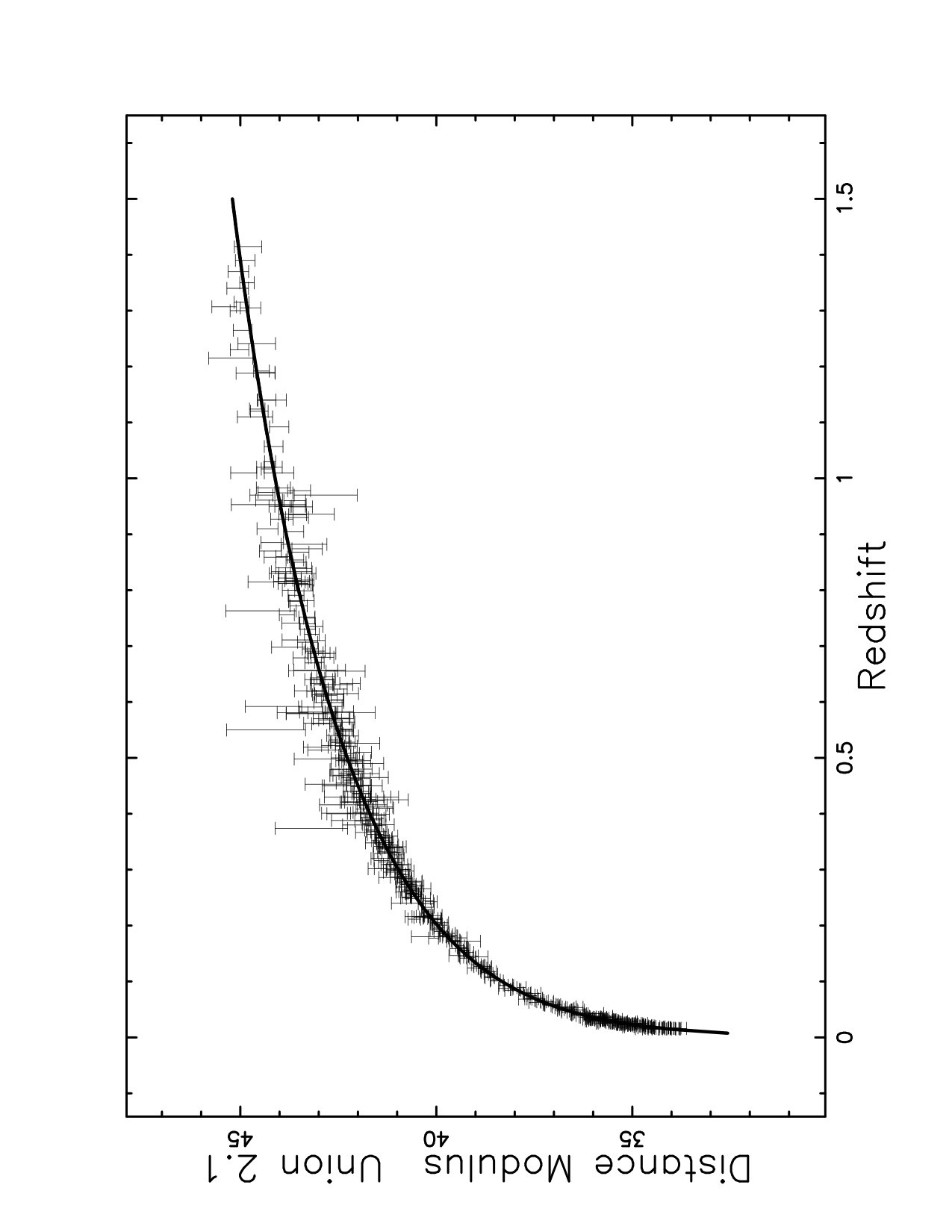 Figure 1
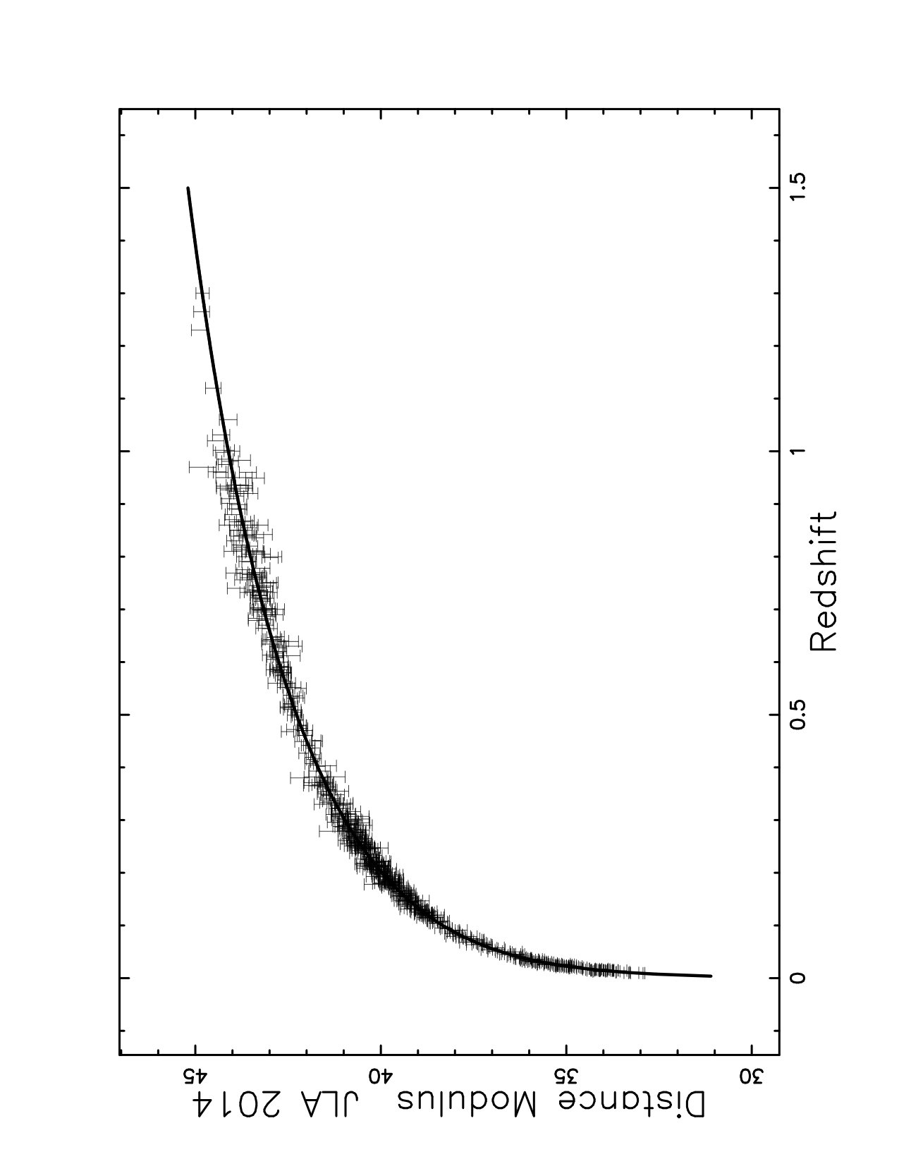 Figure 2
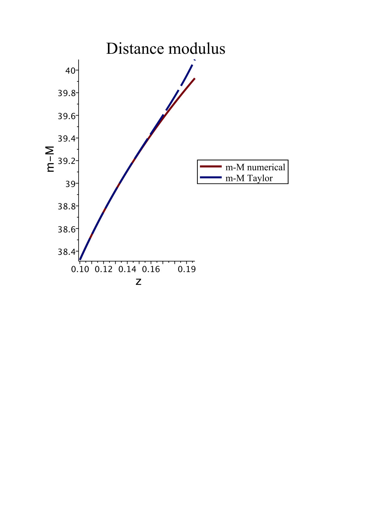 Figure 3
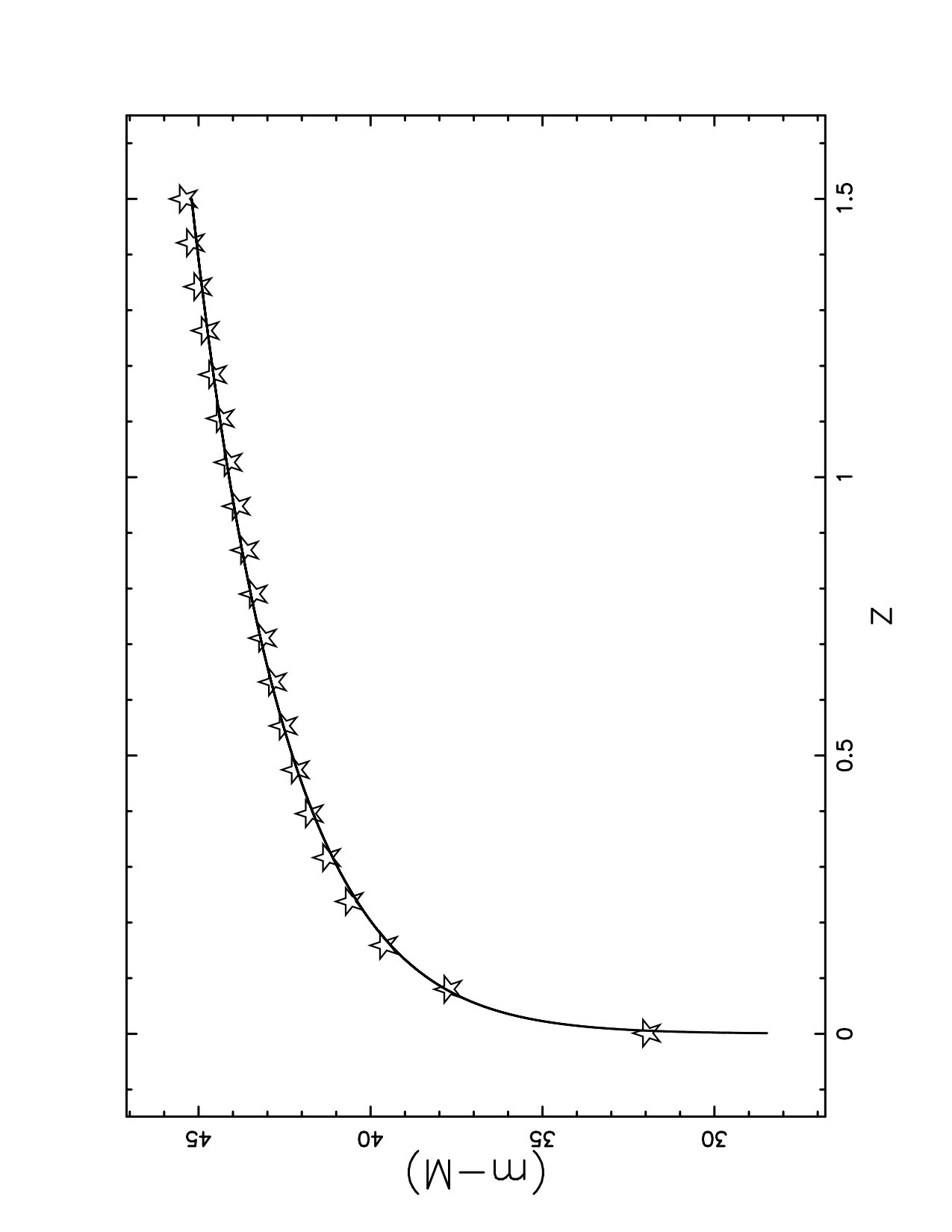 Figure 4
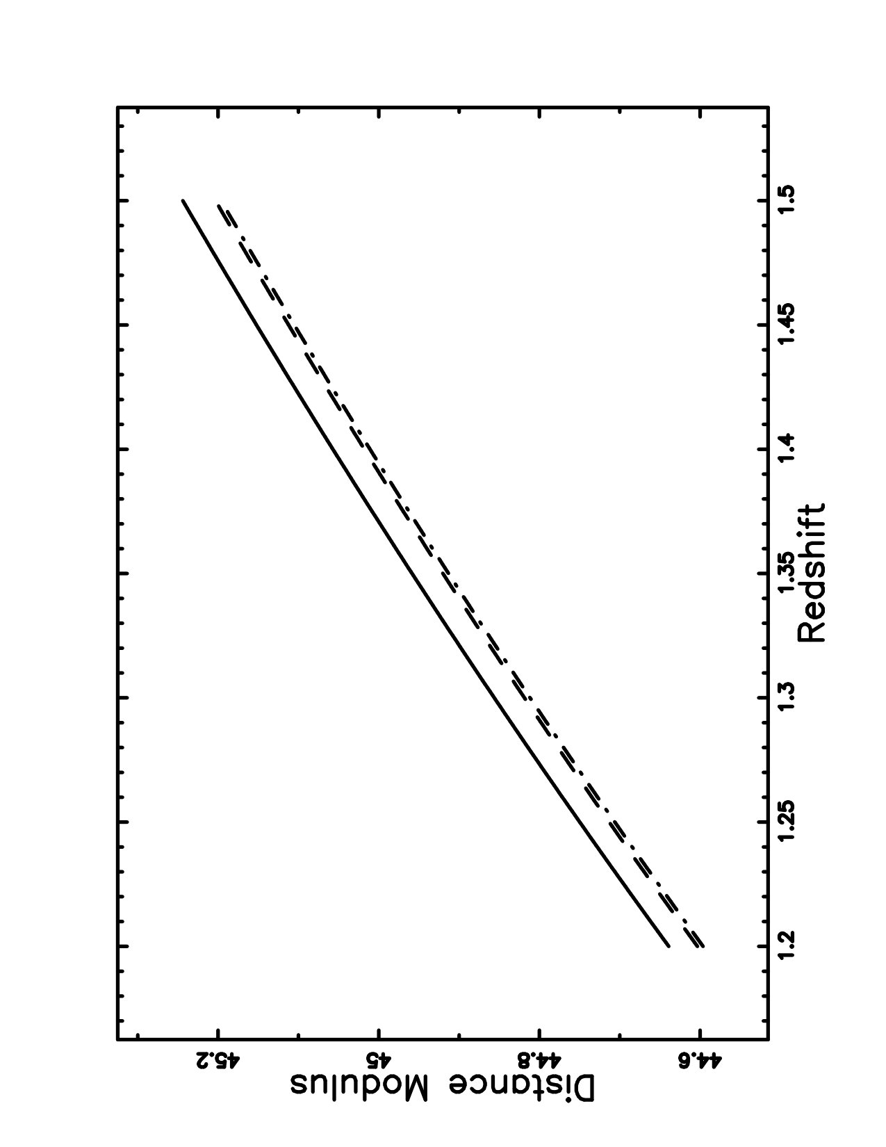 Figure 5
| Cosmology | SNs | parameters | ||||
|---|---|---|---|---|---|---|
| flat-FLRW | 580 | 2 | ; | 562.55 | 0.9732 | 0.66 |
| flat-FLRW-1 | 580 | 1 | ; | 563.52 | 0.9732 | 0.669 |
| CDM | 580 | 3 | = 69.81; ; | 562.61 | 0.975 | 0.658 |
| Cosmology | SNs | parameters | ||||
|---|---|---|---|---|---|---|
| flat-FLRW | 740 | 2 | ; | 627.91 | 0.85 | 0.998 |
| Name | value |
|---|---|
| maximum error | 2.28881836 |
| a | 0.981622279 |
| b | 19.6473351 |
| c | 1.08210218 |
| d | 0.0309164915 |
| e | 0.462291896 |
Peer Reviews
No public reviews on file for this paper yet. If you reviewed it on a platform where reviews are public (OpenReview, ICLR, NeurIPS, ICML), you can paste yours below so the community can read it here.
Videos
No videos yet. Explain this paper in a talk, walkthrough, or lecture? Add one.
A new analytical solution for the distance modulus in flat cosmology
Lorenzo Zaninetti
Physics Department, via P.Giuria 1,
I-10125 Turin,Italy
Abstract
A new analytical solution for the luminosity distance in flat CDM cosmology is derived in terms of elliptical integrals of first kind with real argument. The consequent derivation of the distance modulus allows evaluating the Hubble constant, , and the cosmological constant, .
Keywords : galaxy groups, clusters, and superclusters; large scale structure of the Universe; Cosmology
1 Introduction
The release of two catalogs for the distance modulus of Supernova (SN) of type Ia, namely, the Union 2.1 compilation, see [1], and the joint light-curve analysis (JLA), see [2], allows matching the observed distance modulus with the theoretical distance modulus of various cosmologies. In this fitting procedure, the cosmological parameters are derived in a scientific and reproducible way.
We now focus our attention on the flat Friedmann-Lemaître-Robertson-Walker (flat-FLRW) cosmology. A first fitting formula has been derived by [3] and an approximate solution in terms of Padé approximant has been introduced by [4]. The presence of the elliptical integrals of the first kind in the integral for the luminosity distance in flat-FLRW cosmology has been noted by [5, 6, 7]. As a practical example the luminosity distance can be expanded into a series of orthonormal functions and the two cosmological parameters turn out to be and , see [8]. This paper first introduces in Section 2 a framework useful to build a new solution for the luminosity distance in flat-FLRW cosmology, which will be derived in Section 3.
2 Preliminaries
This section reviews the adopted statistical framework, the CDM cosmology, and an existing solution for the luminosity distance in flat-FLRW cosmology.
2.1 The adopted statistics
In the case of the distance modulus, the merit function is
[TABLE]
where is the number of SNs, is the observed distance modulus evaluated at redshift , is the error in the observed distance modulus evaluated at , and is the theoretical distance modulus evaluated at , see formula (15.5.5) in [9]. The reduced merit function is
[TABLE]
where is the number of degrees of freedom, is the number of SNs, and is the number of parameters. Another useful statistical parameter is the associated -value, which has to be understood as the maximum probability of obtaining a better fitting, see formula (15.2.12) in [9]:
[TABLE]
where GAMMQ is a subroutine for the incomplete gamma function.
The goodness of the approximation in evaluating a physical variable is evaluated by the percentage error
[TABLE]
where is an approximation of .
2.2 The standard cosmology
We follow [10], where the Hubble distance is defined as
[TABLE]
The first parameter is
[TABLE]
where is the Newtonian gravitational constant and is the mass density at the present time. The second parameter is
[TABLE]
where is the cosmological constant, see [11]. These two parameters are connected with the curvature by
[TABLE]
The comoving distance, , is
[TABLE]
where is the ‘Hubble function’
[TABLE]
The above integral does not have an analytical solution but a solution in terms of Padé approximant has been found, see [12].
2.3 A first formula for a flat-FLRW universe
The first model starts from equation (2.1) in [4] for the luminosity distance, ,
[TABLE]
where is the Hubble constant expressed in , is the speed of light expressed in , is the redshift and is the scale-factor. The indefinite integral, , is
[TABLE]
The solution is in terms of , the Legendre integral or incomplete elliptic integral of the first kind, and is given in [13].
The luminosity distance is
[TABLE]
where means the real part. The distance modulus is
[TABLE]
3 A new formula for a flat-FLRW universe
The second model for the flat cosmology starts from equation (1) for the luminosity distance in [14]
[TABLE]
The above formula can be obtained from formula (9) for the comoving distance inserting and the variable of integration, , denotes the redshift.
A first change in the parameter introduces
[TABLE]
and the luminosity distance becomes
[TABLE]
The following change of variable, , is performed for the luminosity distance which becomes
[TABLE]
Up to now we have followed [14] which continues introducing a new function ; conversely we work directly on the resulting integral for the luminosity distance: which is
[TABLE]
where is given by Eq. (16) and is Legendre’s incomplete elliptic integral of the first kind,
[TABLE]
see [15]. The distance modulus is
[TABLE]
and therefore
[TABLE]
where
[TABLE]
and
[TABLE]
with as defined by Eq. (16).
3.1 Data Analysis
In recent years, the extraction of the cosmological parameters from the distance modulus of SNs has become a common practice, see among others [8, 16, 17]. The best fit to the distance modulus of SNs is here obtained by implementing the Levenberg–Marquardt method (subroutine MRQMIN in [9]). This method requires the fitting function, in our case Eq. (22), as well the first derivative , which has a simple expression, and the first derivative , which has a complicated expression. A simplification can be introduced by imposing a fiducial value for the Hubble constant, namely , see [18, 2]. We call this model ‘flat-FLRW-1’, where the ‘1’ stands for there being one parameter. Table 1 presents and for the Union 2.1 compilation of SNs and Figure 1 displays the best fit. The reading of this table allows to evaluate the goodness of the approximation, see (4), in the derivation of the Hubble constant in going from the supposed true value () to the deduced value (), which is . The JLA compilation is available at the Strasbourg Astronomical Data Centre (CDS), and consists of 740 type I-a SNs for which we have the heliocentric redshift, , the apparent magnitude in the B band, the error in , , the parameter , the error in , , the parameter , the error in , , and . The observed distance modulus is defined by equation (4) in [2]:
[TABLE]
The adopted parameters are , and
[TABLE]
see line 1 in Table 10 of [2]. The uncertainty in the observed distance modulus, , is found by implementing the error propagation equation (often called the law of errors of Gauss) when the covariant terms are neglected, see equation (3.14) in [19],
[TABLE]
The parameters as derived from the JLA compilation are presented in Table 2 and the fit is presented in Figure 2.
As an example the luminosity distance for the Union 2.1 compilation with data as in the first line of Table 1 is
[TABLE]
and the distance modulus is
[TABLE]
We now derive some approximate results without Legendre integral for the flat-FLRW case and Union 2.1 compilation with data as in Table 1, first line. A Taylor expansion of order 6 around =0 of the luminosity distance as given by Eq. (19) for the flat-FLRW case and Union 2.1 compilation gives
[TABLE]
The upper limit in redshift, 0.197, is the value for which the percentage error , see equation (4), is . The asymptotic expansion of the luminosity distance with respect to the variable to order 5 for the flat-FLRW case and Union 2.1 compilation gives
[TABLE]
At the lower limit of the percentage error is . The two above approximations at low and high redshift have a limited range of existence but does not contain the Legendre integral as solutions (28) and (29) which cover the overall range .
A Taylor expansion of order 6 of the distance modulus as given by Eq. (22) around for the flat-FLRW case and Union 2.1 compilation gives
[TABLE]
The upper limit in redshift, 0.197, is the value at which the percentage error is . Figure 3 reports both the numerical and the Taylor expansion of distance modulus in the above range.
The asymptotic expansion of the distance modulus with respect to the variable to order 5 for the flat-FLRW case and Union 2.1 compilation gives
[TABLE]
The lower limit in redshift, 1.27, is the value at which the percentage error is . The ranges of existence in for the analytical approximations here derived have the percentage error , see Eq. (4).
We now introduce the best minimax rational approximation, see [20, 21, 15], of degree (2, 1) , for the distance modulus ,
[TABLE]
In the case in which the distance modulus is represented by Eq. (29) and given the interval , the coefficients of the best minimax rational approximation are presented in Table 3; the maximum error for the fit is . Figure 4 displays the data and the fit.
4 Conclusions
We have presented an analytical approximation for the luminosity distance in terms of elliptical integrals with real argument. The fit of the distance modulus of SNs of type Ia allows finding the parameters and for the two compilations in flat-FLRW cosmology
[TABLE]
A first comparison with [8] in the case of the Union 2.1 compilation gives a percentage error for the derivation of and for the derivation of . A second comparison can be done with equation (13) in [22]
[TABLE]
In the case of the Union 2.1 compilation, the percentage error for the derivation of and for . A Taylor expansion at low redshift and an asymptotic expansion are presented both for the luminosity distance and the distance modulus. A simple version of the distance modulus is determined through the best minimax rational approximation. Adopting the cosmological parameters found here, the cosmological constant turns out to be, for the Union 2.1 compilation,
[TABLE]
or introducing and the Planck time, ,
[TABLE]
The statistical parameters of the fits are given in Tables 1 and 2 where the other two models are presented. The values of the in the above table say that for the Union 2.1 compilation the flat cosmology produces a better fit than the CDM does, but the situation is the reverse for the JLA compilation. As a concluding remark we point out that, thanks to the calibration on the distance modulus of SNs, the differences between the solutions here analyzed are minimum. Therefore a restricted range in redshift should be adopted in order to visualize the diverseness, see Figure 5.
The reference list from the paper itself. Each links out to its DOI / PubMed record.
- 1[1] Suzuki N, Rubin D, Lidman C, Aldering G, Amanullah R, Barbary K and Barrientos L F 2012 The Hubble Space Telescope Cluster Supernova Survey. V. Improving the Dark-energy Constraints above z greater than 1 and Building an Early-type-hosted Supernova Sample Ap J 746 85
- 2[2] Betoule M, Kessler R, Guy J and Mosher J 2014 Improved cosmological constraints from a joint analysis of the SDSS-II and SNLS supernova samples A&A 568 A 22
- 3[3] Pen U L 1999 Analytical Fit to the Luminosity Distance for Flat Cosmologies with a Cosmological Constant Ap JS 120 , 49
- 4[4] Adachi M and Kasai M 2012 An Analytical Approximation of the Luminosity Distance in Flat Cosmologies with a Cosmological Constant Progress of Theoretical Physics 127 , 145
- 5[5] Eisenstein D J 1997 An Analytic Expression for the Growth Function in a Flat Universe with a Cosmological Constant Ar Xiv Astrophysics e-prints ( Preprint astro-ph/9709054 )
- 6[6] Liu D Z, Ma C, Zhang T J and Yang Z 2011 Numerical strategies of computing the luminosity distance MNRAS 412 , 2685 ( Preprint 1008.4414 )
- 7[7] Mészáros A and Řípa J 2013 A curious relation between the flat cosmological model and the elliptic integral of the first kind A&A 556 A 13
- 8[8] Benitez-Herrera S, Ishida E E O, Maturi M, Hillebrandt W, Bartelmann M and Röpke F 2013 Cosmological parameter estimation from SN Ia data: a model-independent approach MNRAS 436 , 854 ( Preprint 1308.5653 )