Compiler-assisted Adaptive Program Scheduling in big.LITTLE Systems
Marcelo Novaes, Vin\'icius Petrucci, Abdoulaye Gamati\'e, Fernando, Quint\~ao

TL;DR
This paper introduces Astro, a compiler-assisted adaptive scheduling system for big.LITTLE architectures that leverages program structure and reinforcement learning to optimize hardware configuration, outperforming existing schedulers.
Contribution
It presents a novel approach combining compiler analysis and reinforcement learning to improve program scheduling in heterogeneous architectures.
Findings
Astro outperforms GTS on Rodinia and Parsec benchmarks.
Using program phases improves scheduling decisions.
Reinforcement learning effectively maps program features to hardware configs.
Abstract
Energy-aware architectures provide applications with a mix of low (LITTLE) and high (big) frequency cores. Choosing the best hardware configuration for a program running on such an architecture is difficult, because program parts benefit differently from the same hardware configuration. State-of-the-art techniques to solve this problem adapt the program's execution to dynamic characteristics of the runtime environment, such as energy consumption and throughput. We claim that these purely dynamic techniques can be improved if they are aware of the program's syntactic structure. To support this claim, we show how to use the compiler to partition source code into program phases: regions whose syntactic characteristics lead to similar runtime behavior. We use reinforcement learning to map pairs formed by a program phase and a hardware state to the configuration that best fit this setup. To…
Click any figure to enlarge with its caption.
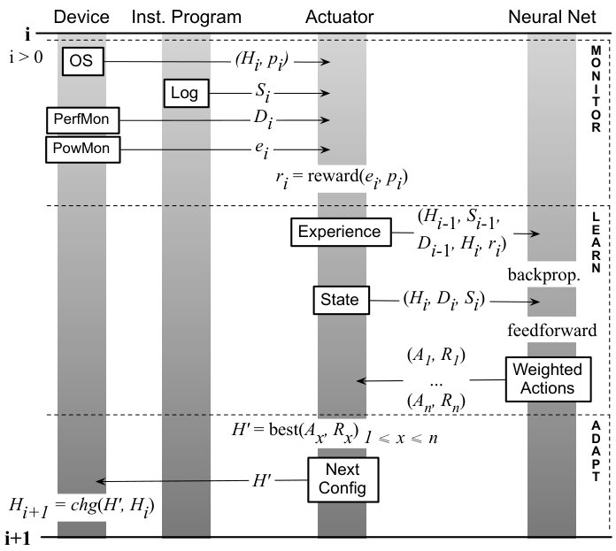 Figure 1
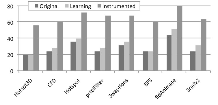 Figure 2
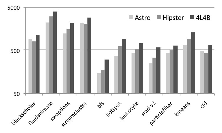 Figure 3
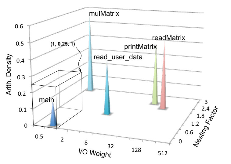 Figure 4
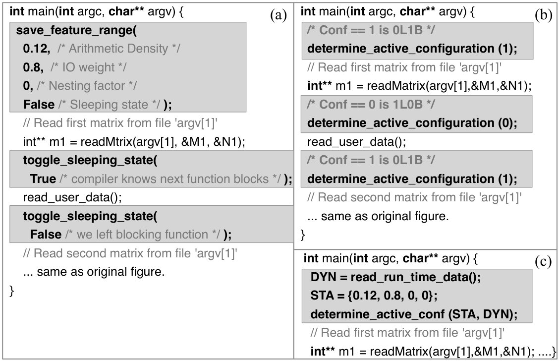 Figure 5
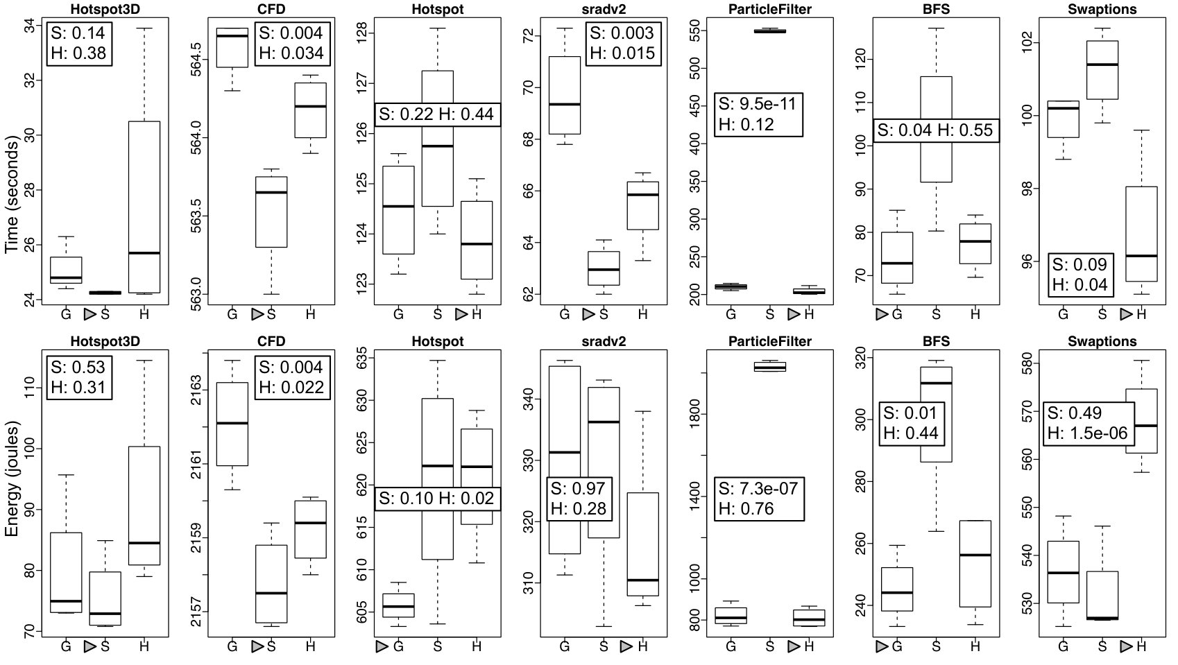 Figure 6
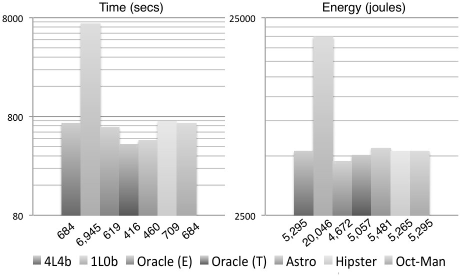 Figure 7
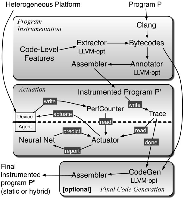 Figure 8
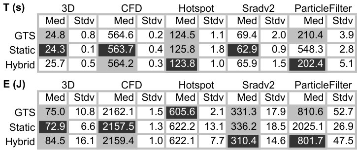 Figure 9
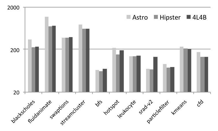 Figure 10
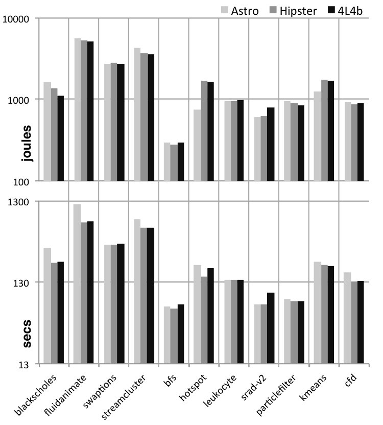 Figure 11
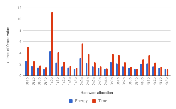 Figure 12
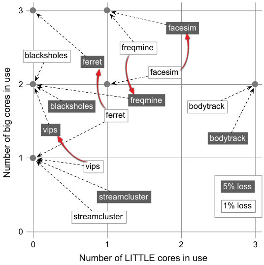 Figure 13
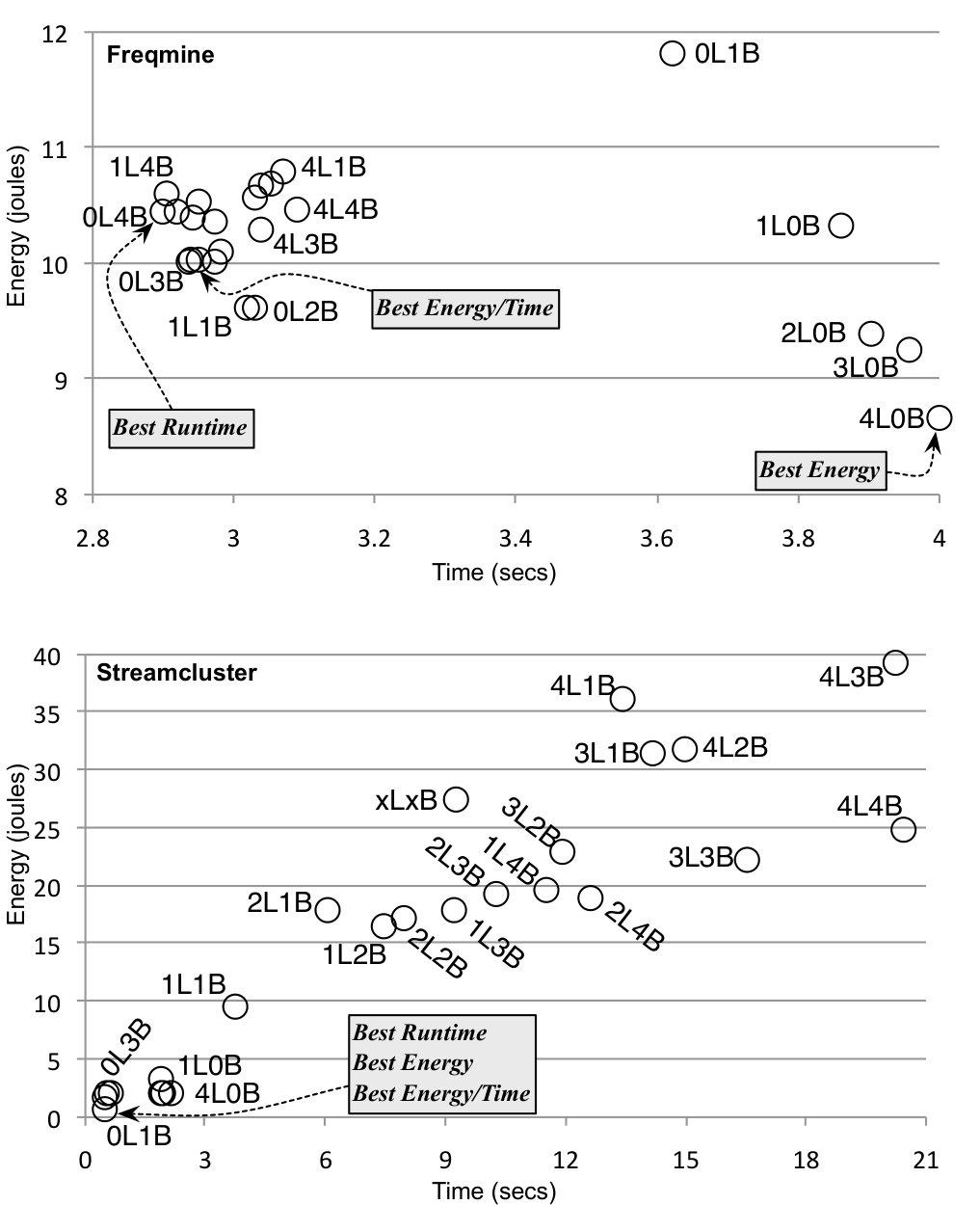 Figure 14
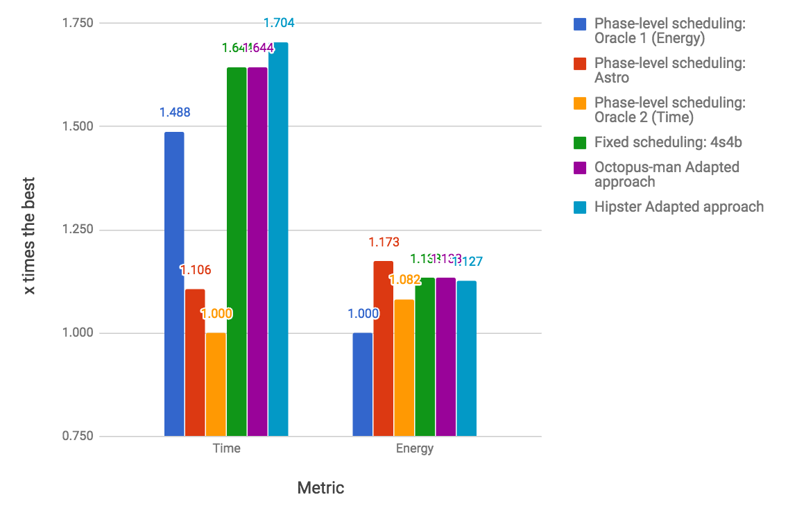 Figure 15
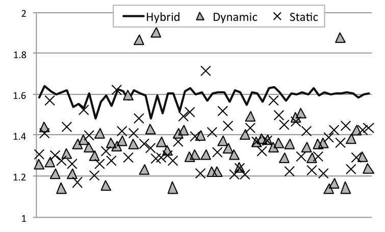 Figure 16
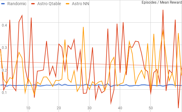 Figure 17
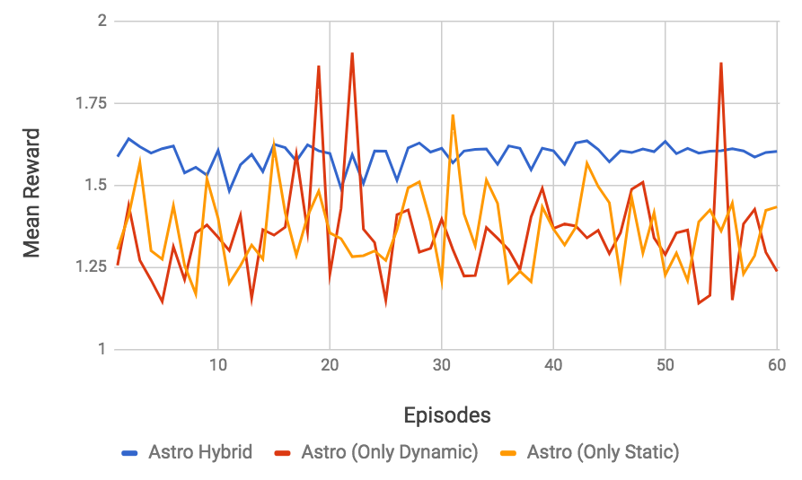 Figure 18
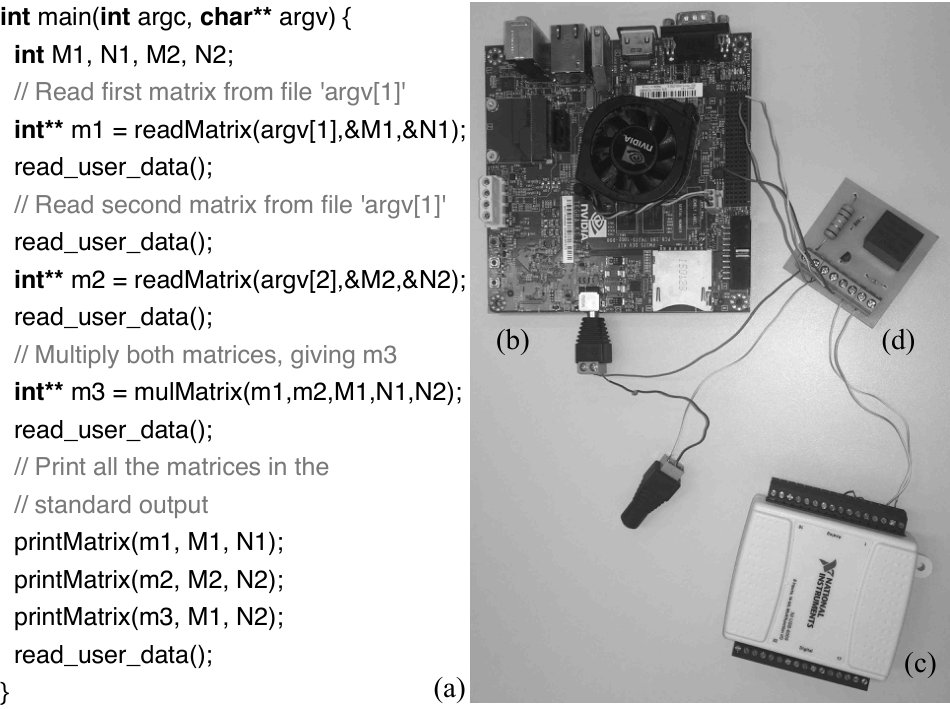 Figure 19
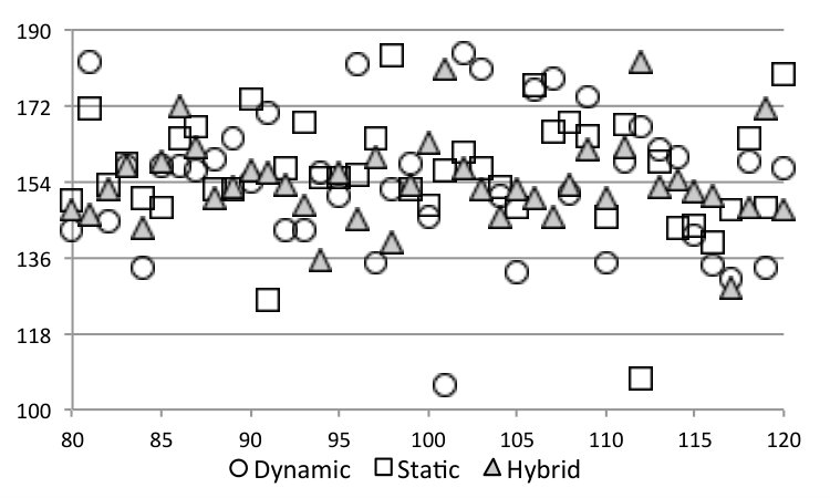 Figure 20
 Figure 21
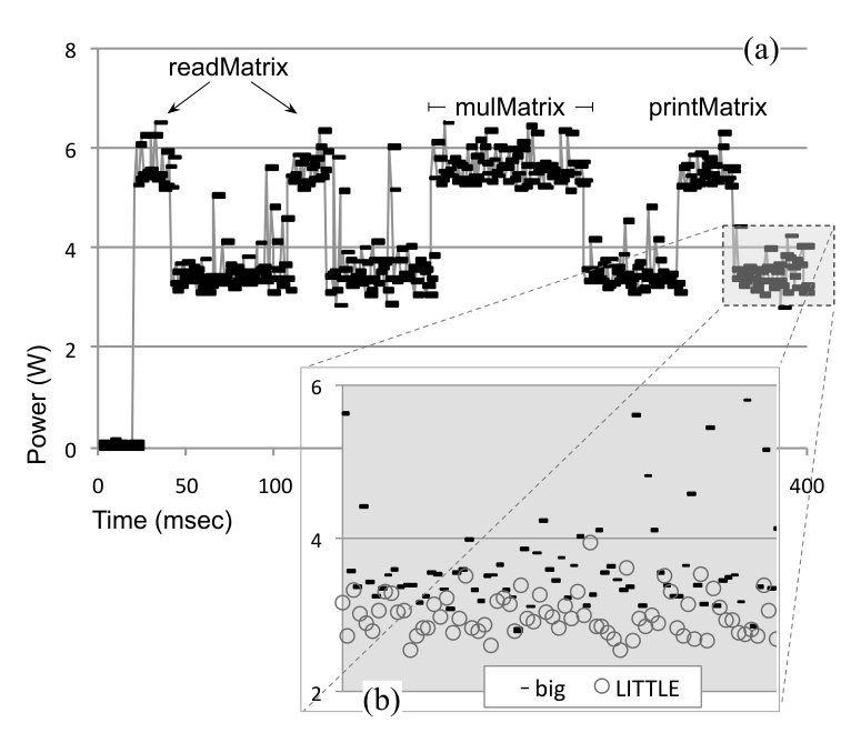 Figure 22
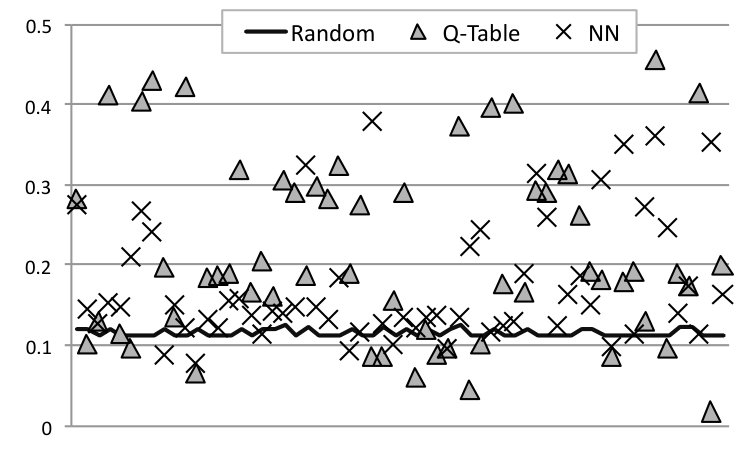 Figure 23
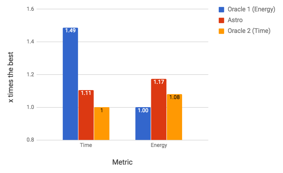 Figure 24
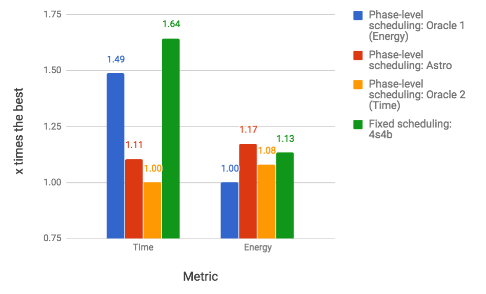 Figure 25
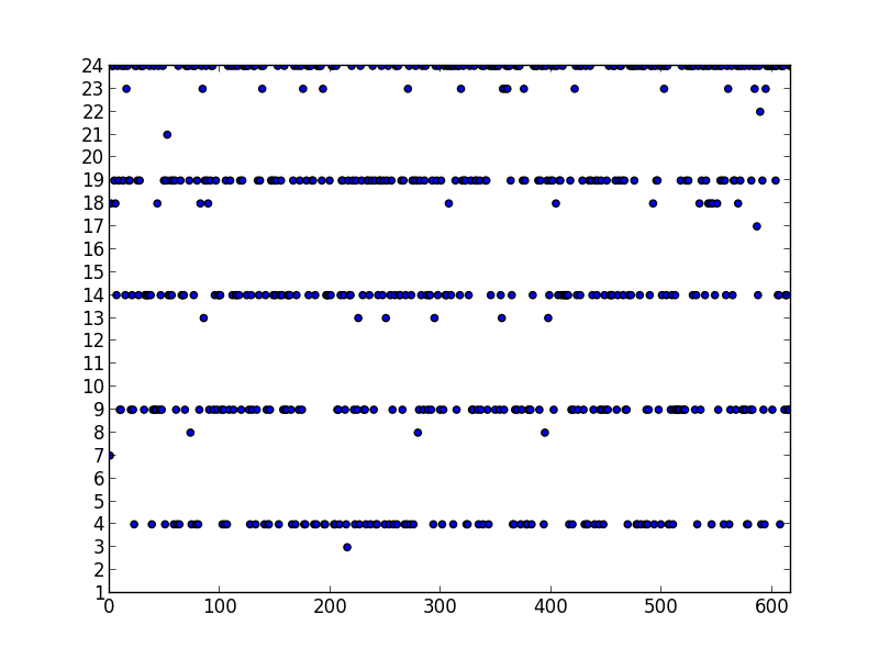 Figure 26
 Figure 27
 Figure 28
| Work | Level | Source | Auto | Runtime | Learn |
|---|---|---|---|---|---|
| (Poesia et al., 2017) | C | Yes | Yes | No | Yes |
| (Barik et al., 2016) | C | Yes | Yes | Yes | No |
| (Rossbach et al., 2013) | C/L | Yes | No | Yes | No |
| (Luk et al., 2009) | C/L | Yes | No | Yes | No |
| (Joao et al., 2012) | A/L | Yes | No | No | No |
| (Lukefahr et al., 2016) | A | No | Yes | No | No |
| (Van Craeynest et al., 2012) | A | No | Yes | No | No |
| (Nishtala et al., 2017) | O | No | Yes | Yes | Yes |
| (Petrucci et al., 2015) | O | No | Yes | Yes | No |
| (Augonnet et al., 2011) | L | Yes | No | No | No |
| (Piccoli et al., 2014) | O/C | Yes | Yes | Yes | No |
| (Tang et al., 2013) | O/C | Yes | Yes | Yes | No |
| (Cong and Yuan, 2012) | O/C | Yes | Yes | Yes | No |
| Astro | O/C | Yes | Yes | Yes | Yes |
Peer Reviews
No public reviews on file for this paper yet. If you reviewed it on a platform where reviews are public (OpenReview, ICLR, NeurIPS, ICML), you can paste yours below so the community can read it here.
Videos
No videos yet. Explain this paper in a talk, walkthrough, or lecture? Add one.
Taxonomy
TopicsParallel Computing and Optimization Techniques · Cloud Computing and Resource Management · Advanced Data Storage Technologies
1
Compiler-assisted Adaptive Program Scheduling in big.LITTLE Systems
Marcelo Novaes
Department of Computer ScienceUFMGBrazil
,
Vinícius Petrucci
Department of Computer ScienceUFBABrazil
,
Abdoulaye Gamatié
LIRMMCNRSFrance
and
Fernando Quintão
Department of Computer ScienceUFMGBrazil
Abstract.
Energy-aware architectures provide applications with a mix of low (LITTLE) and high (big) frequency cores. Choosing the best hardware configuration for a program running on such an architecture is difficult, because program parts benefit differently from the same hardware configuration. State-of-the-art techniques to solve this problem adapt the program’s execution to dynamic characteristics of the runtime environment, such as energy consumption and throughput. We claim that these purely dynamic techniques can be improved if they are aware of the program’s syntactic structure. To support this claim, we show how to use the compiler to partition source code into program phases: regions whose syntactic characteristics lead to similar runtime behavior. We use reinforcement learning to map pairs formed by a program phase and a hardware state to the configuration that best fit this setup. To demonstrate the effectiveness of our ideas, we have implemented the Astro system. Astro uses Q-learning to associate syntactic features of programs with hardware configurations. As a proof of concept, we provide evidence that Astro outperforms GTS, the ARM-based Linux scheduler tailored for heterogeneous architectures, on the parallel benchmarks from Rodinia and Parsec.
big.LITTLE architecture, Adaptation, Compiler
††conference: ; ††journalyear: ;††isbn: ††doi: ††copyright: none††ccs: Software and its engineering General programming languages††ccs: Social and professional topics History of programming languages
1. Introduction
Contemporary hardware found in mobile phones and data centers sport multiple ways to reduce energy consumption. Two of these techniques are the combination of low and high power cores (the so called big.LITTLE architectures) (Chung et al., 2012), and the ability to adjust power and speed dynamically (DVFS) (Le Sueur and Heiser, 2010). This design gives us the possibility to allocate to each parallel application the hardware configuration that best suits it. A hardware configuration consists of a number of cores, their type and their frequency level. We say that a configuration suits a program better than another configuration if runs said program more efficiently than , according to some metric such as runtime or energy consumption. Nevertheless, even though we have today the possibility of choosing among several configurations, the one that better fits the needs of a certain program, we still have no clear technique to perform this choice seamlessly.
We call the task of allocating parts of a parallel program to processors the code placement problem. State-of-the-art approaches solve this problem dynamically or statically. Dynamic solutions (Margiolas and O’Boyle, 2016; Nishtala et al., 2017; Petrucci et al., 2015) are implemented at the runtime level, at the operating system, or via a middleware. Static approaches (Grewe and O’Boyle, 2011; Mendonça et al., 2017; Nugteren and Corporaal, 2014; Verdoolaege et al., 2013) are implemented at the compiler level. The main advantage of the dynamic approach is the fact that it can use runtime information to weight the choices it makes. Static techniques, in turn, provide reduced runtime cost and better leverage of program characteristics. In this paper, we claim that it is possible to join these two approaches, achieving a synergy that, otherwise, could not be attained by each technique individually.
To fundament this claim, we start from a technique that has been proven effective to schedule computations in big. LITTLE architectures: Reinforcement learning. Nishtala et al. (Nishtala et al., 2017) showed that reinforcement learning helps to find good hardware configurations to applications subject to varying dynamic conditions. The beauty of this approach is adaptability: it provides the means to explore a vast universe of states, formed by different hardware setups and runtime data changing over time. Given enough time, well-tuned heuristics find a set of scheduling decisions that suits the underlying hardware. Yet, “enough time” can be too long. The universe of runtime states is unbounded, and program behavior is hard to predict without looking into its source code. To speedup convergence, we resort to the compiler.
The compiler gives us two benefits. First, it lets us mine program features, which we can use to train the learning algorithm. Second, it lets us instrument the program. This instrumentation allows the program itself to provide feedback to the scheduler, concerning the code region currently under execution. Based on previous knowledge, collected statically, about characteristics of that region, the scheduler can take immediate action. An action consists in choosing a new state to represent program behavior, and collecting the reward related to that choice. Such feedback is then used to fine-tune and improve scheduling decisions. As we show in Section 4, convergence is faster, and runtime shorter.
To validate our ideas, we have materialized them into a framework to instrument and execute applications in heterogeneous architectures: the Astro System. Astro collects syntactic characteristics from programs and instruments them using LLVM (Lattner and Adve, 2004). Experiments in programs from Parsec (Bienia et al., 2008) and Rodinia (Che et al., 2009) running on an Odroid XU4 show that we can obtain speedups of more than 10% over the default GTS scheduler used in ARM-based systems. Such numbers result from the following contributions:
**Observations:: **
in Section 2, we demonstrate that the performance of a program running on a heterogeneous architecture vary depending on which part of its text we consider. This observation points us to the key insight: the possibility of augmenting an adaptive runtime apparatus with awareness of program characteristics.
**Compiler:: **
in Section 3.1, we explain how to collect and discretize program features, and in Section 3.2, we explain how to instrument a program, so to use said features to fine-tune an adaptive code placement algorithm.
**Runtime:: **
in Section 3.3, we show how to integrate the static information that we collect with an adaptive runtime environment. Once we train a program, we generate code that maps different parts of it to suitable hardware configurations.
2. Empirical Observations
This section motivates our work through three empirical observations. First, different hardware configurations yield very different tradeoffs between power consumption and runtime speed for a program (Figure 1). Second, this behavior happens because programs have power phases: depending on the operations that they perform, they might consume more or less power per time unit (Figure 2). Third, the best hardware configuration for a program might not suit the needs of a different application (Figure 4). Central to the discussion in this section is the notion of a hardware configuration:
Definition 2.1 (Hardware Configuration).
A heterogeneous architecture is formed by a set of processors. A hardware configuration is a function . If , then processor is said to be active in , otherwise it is said to be inactive.
First Observation. The same application might benefit differently from different hardware configurations. This benefit is measured in terms of processing time and energy consumption. Figure 1 shows how two benchmarks from the PARSEC suite – Freqmine and Streamcluster – fare on an Odroid XU4 board featuring 4 Cortex-A15 2.0Ghz cores and 4 Cortex-A7 1.4Ghz cores. Following a nomenclature adopted by ARM, we shall call the A15 cores bigs, and the A7 cores LITTLEs. By switching on and off the different cores, we have 24 different hardware configurations111We have configurations, because we do not count the setup in which all cores are off.
Each dot in the figure represents the average of 10 executions on the same configuration, using the smallest222This experiment would take 12 days using the largest inputs. input available in PARSEC. Variance is almost negligible, staying under 1% in every sample, for the two benchmarks. The X-axis shows the sum of the execution times of processors active in a particular configuration; hence, it is not clock time. Energy is measured with the Odroid XU3 on-board power measurement circuit and refers to work performed within the processors only; thus, peripherals are not considered.
Figure 1 lets us conclude that the energy and runtime footprint of applications vary greatly across different hardware configurations. For instance, the most time efficient configuration for Freqmine is 0L4B, i.e., four bigs and no LITTLEs (2.90secs, 10.43J). However, the most energy efficient configuration is 4L0B (4.01secs, and 8.65J). Results are not the same for Streamcluster. The best energy configuration is 0L1B (0.48secs, 0.69J). This is also the most time efficient configuration. Freqmine shows more parallelism than Streamcluster; therefore, it benefits more from a larger number of cores. This diversity of scenarios happen because programs have phases. Energy and runtime behavior are similar within the same phase, and potentially different across different phases.
Second Observation. The instantaneous power consumed by a program is not always constant. In other words, a program has power phases. Figure 2 (a) shows a program which we have crafted to emphasize the different phases that a program undergoes during its execution. This program performs the following actions: (i) read two matrices from text files; (ii) multiply them and (iv) prints all the matrices in the standard output. In between each of these actions we have interposed commands to read data from the standard input.
Figure 3 shows the power profile of this program. This chart has been produced with JetsonLeap (Bessa et al., 2016), an apparatus that let us measure the energy consumed by programs running on the Nvidia TK1 Jetson board333In this section we use two different experimental setups: Odroid XU4 and Tegra TK1. The former gives us the richness of configurations seen in Figure 1. This diversity is absent on the latter, that has only one LITTLE core. However, the TK1 board gives us access to JetsonLeap, and, consequently, the ability to measure energy per programming events.. JetsonLeap is formed by three components: the target Nvidia board (Figure 2 (b)), a data acquisition device, which reads the instantaneous power consumed by the board (Figure 2 (c)), and a synchronization circuit, which lets us communicate to the power meter which program event is running at each instant (Figure 2 (c)).
Distinct phases exist within the same program because it might use the hardware resources differently, depending on which part of it is running. By reading performance counters, we know that during matrix multiplication, CPU is at is maximum usage. During the input/output operations, this utilization drops slightly, and other components of the hardware, such as its serial port, are more exercised instead. This fall is steep once the program is waiting for user inputs. The CPU is not the only hardware component that accounts for power dissipation. The JetsonLeap apparatus measure energy for the entire hardware. Thus, the under utilization of the CPU does not mean that overall power consumption will decrease. Nevertheless, variations in the CPU usage are likely to cause variations in the power profile of the program.
Discovering such program phases by means of purely dynamic techniques is possible, yet difficult. As we shall demonstrate in Section 4, we can use profiling techniques, à la Hipster (Nishtala et al., 2017), to identify variations in program behavior. However, this approach has two shortcomings. First, distinct program parts, with very different resource demands in terms of memory, CPU, disk and such, can display similar dynamic characteristics. For instance, we could imagine a scenario in which function read_user_data, in Figure 2 is implemented via busy waiting. In this case, instead of the valleys observed in Figure 3, we would encounter a power line similar to that produced by CPU-intensive functions like mulMatrix. Second, profiling-based techniques face a tradeoff between precision and overhead. Fast detection asks for high sampling rates; thus burdening the application which originally we intended to optimize. On the other hand, purely static approaches are not better either. Although likely to yield lower adaptation overhead, they fail to account for information only available at runtime such as varying input sizes. For instance, a static scheduler might decide always run mulMatrix and read_user_data in different configurations. However, when operating on matrices that are too small, the cost of changing the hardware configuration might already overshadow the possible gains available through more parsimonious usage of the architecture’s resources.
Third Observation. The best architecture configuration, in terms of runtime or energy consumption, differs among programs. Figure 4 shows the best configurations that we have found on the Odroid XU4 setup, for six PARSEC applications. We define the best configuration as the one that spends less energy, given a certain slowdown compared to the fastest configuration. Clearly, there is not a single winner. Configurations vary among programs, and even within the same program, given different acceptable slowdowns.
In the rest of this paper, we shall describe a general methodology, henceforth called the Astro system, which mixes static and dynamic analyses, to find good hardware configurations for the functions invoked during the execution of a program. In this section, we have highlighted key motivation behind our design: (i) a modern heterogeneous hardware exposes a number of different configurations that is too large to be evaluated manually; (ii) a program presents power phases, which can be more easily detected by methods that are aware of structural properties of the code. Thus, we claim that effective adaptation demands knowledge of program characteristics. Such information is readily available to the compiler; however, it is hard to be precisely acquired by techniques unaware of the program’s structure.
3. The Astro System
This section describes the design and implementation of our approach to solve the problem of finding good hardware configurations for programs. We state this problem as follows:
Definition 3.1.
Scheduling of Programs in Heterogeneous Architectures* (SPha)
Input: a program , its input , hardware configurations , energy threshold , and performance threshold .
Output: , a new version of , which switches between configurations, and process using % less energy, with a slowdown of no more than %.*
In this paper, we solve SPha using an assortment of techniques, which give us the means to generate code that is well adapted to different architectures and workloads. Figure 5 provides a general overview of these techniques, emphasizing the different stages over which we go in the process of solving SPha. Section 3.1 describes program instrumentation, a necessary step to partition a program into phases. Section 3.2 goes over actuation; and Section 3.3 discusses the generation of the final program. However, before we move into the particulars of our solution to SPha, we provide a brief introduction to Q-Learning, the flavour of reinforcement learning that we have adopted.
Q-Learning.
Q-learning is a reinforcement learning algorithm (Sutton and Barto, 1998). Given some notion of state (Definition 3.2) and reward (Definition 3.7), it finds an optimized policy to perform the best action (Definition 3.9). Q-learning is attractive because there is no need to know in advance the precise results of the actions before we perform them; that is, we learn about the environment as we perform actions on it. A Markov Decision Process (MDP) drives Q-learning. A MDP is given by a set of states , a set of possible actions , a reward function , and a state transition mapping that describes the effects of taking each action in each state of the environment. The Markov property says that the results of an action depends only on the state where the action was taken, regardless of any other prior states.
3.1. Phase Partitioning
A running program might cause the hardware to go over an infinite number of different states. Because this universe is unbounded, Definition 3.2 discretizes the notion of a State. In that definition, is a Program Phase and is a Hardware Phase. Program phases are discussed in Section 3.1.1, and hardware phases are discussed in Section 3.1.2.
Definition 3.2 (State).
A state is a triple representing a hardware configuration , a program phase and a hardware phase .
3.1.1. Program Phases
Static Program Phases depend only on the syntax of a program. Definition 3.3 formalizes this notion. A static program phase is not equivalent to a program region, because different regions can present the same set of feature ranges. Example 3.4 clarifies the meaning of these definitions.
Definition 3.3 (Program Phase).
A code-level feature (also called code feature or simply feature) is a syntactic characteristic of a program, such as number of n-nested loops or instruction mix. A feature range is a contiguous interval of values that a feature can assume, and that partitions the feature space into equivalence classes. A program phase is a group of feature ranges, covering different features.
Example 3.4.
The density of arithmetic and logical instructions is a code-level feature, which we obtain by dividing the number of such opcodes by the total number of program instructions. We can define different feature ranges covering this metric, such as , and . The number of nested loops yields another feature. In this case, possible ranges are , and . Finally, an expectation on the number of I/O routines called in a function gives us a third feature. A heuristic to estimate it is: , for every I/O call nested into loops. Potential intervals for this metric are , , and . The possible combinations of these ranges gives us 36 program phases. If we collect these features for each function in the program code, then we can map any of them to one of these program phases.
In this paper, we mine (e.g., collect) features from the intermediate program representation that the compiler manipulates before producing executable code. We have implemented a Phase-Extractor using the LLVM compiler. The result of mining program features is a map that assigns phases to program regions. This map depends on the choice of program region. Many different granularities of regions are possible, such as instruction, basic block, loop, Single-Entry-Single-Exit block (Ferrante et al., 1987), etc. We have chosen to work mostly at the granularity of functions. The “mostly” in this case, refers to the fact that we also change phases before and after library calls that cause the program to block waiting for some event (see the Barrier phase, in the discussion that follows). Pragmatically, this amounts to say that the instrumented program adds logic to change phases at the entry point of functions, and around certain library calls.
Example 3.5.
Figure 6 shows the five functions in Figure 2, classified according to features seen in Example 3.4. We are assigning these functions hypothetical values. Because we have three features, we can map them into a three-dimensional space. Each phase corresponds to a cube in this space. Figure 6 shows the sub-space that corresponds to the phase: , and . Function main, in our example, fits in this phase.
Our Choice of Program Phases. In our implementation, we combine four code features to determine program phases. These features are all “densities”, i.e., they represent a certain quantity of instructions normalized by the total of instructions in the target function. We use the following features:
- •
IO-Dens: proportion of library calls that perform I/O operations;
- •
Mem-Dens: proportion of instructions that access memory (loads and stores);
- •
Int-Dens: proportion of arithmetic and logic instructions that operate on integer types.
- •
FP-Dens: proportion of arithmetic and logic instructions that operate on floating point types.
- •
Locks-Dens: proportion of lock instructions.
- •
Barrier: true when the program invokes a multi-thread barrier that forces it to wait for some blocking event.
- •
Net: true when the program invokes a library call that forces it to wait for some network-related event.
- •
Sleep: true when the program invokes a sleep library call that forces it to wait unconditionally.
We have defined four program phases, which appear as combinations of the features above. This choice is arbitrary. We have opted for a simple partitioning, involving only a handful of features for convenience, as this choice already lets us support the main thesis of this paper: that static features greatly enhance the dynamic scheduling of computations in heterogeneous hardware. The program phases that we shall consider in Section 4 are:
- •
Blocked: Barrier = true or Net = true or Sleep = true or Locks-Dens ;
- •
I/O Bound: IO-Dens + Mem-Dens and not(Blocked) and Locks-Dens = 0;
- •
CPU Bound: Int-Dens + FP-Dens and not(Blocked);
- •
Other: in case none of the previous relations hold.
3.1.2. Hardware Phases
While the program phases seen in Section 3.1.1 depend only on syntactic program characteristics, hardware phases depend on the dynamic state of the hardware:
Definition 3.6 (Hardware Phase).
A Performance Counter is any monitor that collects dynamic information about the hardware state, such as CPU performance and cache miss rate. The domain over which the performance counter ranges can be partitioned into phases. Given a collection of performance counters , where each is partitioned into phases, then a hardware phase is any combination within the product .
The monitoring of hardware phases does not require program instrumentation. Instead, an actuator reads the state of hardware performance counters periodically. Modern architectures already provide an array of performance counters that can be queried. In this paper, we consider four kinds of counters to define hardware phases:
- •
IPC: instructions per cycle in the ranges ;
- •
CMA: cache misses per cache accesses in the ranges ;
- •
CMI: cache misses per instruction executed, in the ranges ;
- •
CPU: utilization of the CPU, in the ranges .
Each counter is partitioned in three buckets. Therefore, we consider a total of hardware phases.
3.2. Actuation
The heart of the Astro system is the Actuation Algorithm outlined in Figure 7. Actuation consists of phase monitoring, learning and adapting. These three steps happens at regular intervals, called check points, which, in Figure 7, we denote by i and i+1. The rest of this section describes these events.
3.2.1. Monitoring
To collect information that will be later used to solve SPha, Astro reads four kinds of data. Figure 7 highlights this data:
- •
From the Operating System (OS): current hardware configuration and instructions executed since last check point.
- •
From the Program (Log): the current program phase .
- •
From the device’s performance counters (PerfMon): the current hardware phase .
- •
From the power monitor (PowMon (Walker et al., 2016)): the energy consumed since the last checkpoint.
The monitor collects this data at periodic intervals, whose granularity is configurable. Currently, it is 500 milliseconds. The recording of the program phase is aperiodic, following from instrumentation inserted in the program by the compiler. As discussed in Section 3.1.1, information is logged at the entry point of functions, and around library calls that might cause the program to enter a dormant state. The hardware configuration is updated whenever it changes. The metrics and lets us define the notion of reward as follows:
Definition 3.7 (Reward).
The reward is the set of observable events that determine how well the learning algorithm is adapting to the environment. The reward is computed from a pair , formed by the Energy Consumption Level , measured in Joules per second (Watt), and the CPU Performance Level , measured in number of instructions executed per second.
The metric used in the reward is given by a weighted form of performance per watt, namely , where is a design parameter that gives a boosting performance effect in the system. This is usually a trade-off between the performance and energy consumption. To optimize for energy, we let . A value of emphasizes performance gains: the reward function optimizes (in fact, maximizes the inverse of) the energy delay product per instruction, given by ; letting we have . This aims to minimize both the energy and the amount of time required to execute thread instructions (Brooks et al., 2000).
Example 3.8.
Continuing with Example 3.5, Figure 8 (a) shows the instrumentation of function main (Figure 2) to log program phases.
3.2.2. Learning
The learning phase uses the Q-learning algorithm. As illustrated in Figure 7, a key component in this process is a multi-layer Neural Network (NN) that receives inputs collected by the Monitor. The NN outputs the actions and their respective rewards to the Actuator so that a new system adaptation can be carried out. Following common methodology, learning happens in two phases: back-propagation and feed-forwarding. During back-propagation we update the NN using the experience data given by the Actuator (Figure 7). Experience data is a triple: the current state, the action performed and the reward thus obtained. The state consists of a hardware configuration , static features and dynamic features at check points i-1. The action performed at check point i-1 makes the system move from hardware configuration to . The reward is given by , received after the action is taken. The NN consists of a number of layers including computational nodes, i.e., neurons. The input layer uses one neuron to characterize each triple . The output layer has one neuron per action/configuration available in the system. During the feed-forward phase, we perform predictions using the trained NN. Each node of the NN is responsible to accumulate the product of its associated weights and inputs. Given as input a state at check point i, the result of the feed-forward step is an array of pairs , where is an action, and is its reward, estimated by NN. Actions determine configuration changes; rewards determine the expected performance gain, in terms of energy and time, that we expect to obtain with the change. We use the method of gradient descent to minimize a loss function given by the difference between the reward predicted by the NN, and the actual value found via hardware performance counters.
3.2.3. Adaptating
At this phase, Astro takes an action. Together with states and rewards, actions are one of the three core notions in Q-learning, which we define below:
Definition 3.9 (Action).
Action is the act of choosing the next hardware configuration to be adopted at a given checkpoint.
An action may change the current hardware configuration; hence, adapting the program according to the knowledge inferred by the Neural Network. Following Figure 7, we start this step by choosing, among the pairs , the action associated with the maximal reward . determines, uniquely, a hardware configuration . Once is chosen, we proceed to adopt it. However, the adoption of a configuration is contingent on said configuration being available. Cores might not be available because they are running higher privilege jobs, for instance. If the Next Configuration is accessible, Astro enables it; otherwise, the whole system remains in the configuration active at check point i. Such choice is represented, in Figure 7, by the function . Regardless of this outcome, we move on to the next check point, and to a new actuation round.
3.3. Code Scheduling
After we have trained a program to a given architecture, we imprint this knowledge directly in that program’s code. In Figure 5, this step is named Final Code Generation. Code generation consists in inserting instrumentation into the target program. Instrumentation is inserted in the same regions modified to mark program phases (see Section 3.1.1): at the entry point of functions, and around particular library calls. Example 3.10 illustrates this instrumentation.
Example 3.10.
Figure 8 shows the final actuation code for the program in Figure 2. Function determine_active_configuration tries to move the program to the configuration that has produced the largest rewards for that program phase. We consider two versions of instrumentation: static, as in Figure 8(b), and hybrid, as in Figure 8 (c). The latter can read hardware status to improve the decision making process.
The static scheduling discussed in Example 3.10 always maps the same program region to the same hardware configuration. Hybrid scheduling might change decisions, given enough runtime information. As we show in Section 4, the static scheduling yields lower runtime overhead than Astro’s hybrid scheduling. However, this modus operandi is unable to adapt the program to its workload; and cannot recover from bad decisions. A striking example is the benchmark ParticleFilter (see Fig. 10 in Section 4.2). In this case, even with the runtime overhead, the flexibility of hybrid instrumentation paid off in terms of energy and speed.
4. Evaluation
This section presents an experimental evaluation of the Astro system over several parallel benchmarks running on a big.LITTLE system. In the process of evaluating Astro, we shall provide answers to the following research questions:
- •
RQ1: How close can Astro be from an optimal oracle?
- •
RQ2: How does Astro compare against fixed and immutable best configuration choices?
- •
RQ3: How does Astro compare against state-of-the-art schedulers?
- •
RQ4: How does Astro behave on an actual device?
- •
RQ5: How much does Astro increase code size?
Experimental Setup. We use two experimental setups: program traces, henceforth called simulation; and an actual device, the Odroid XU4. Experiments in Section 4.1 use simulation because they involve testing exhaustively every hardware configuration. Experiments in Section 4.2 run on an actual device: the Odroid XU4 development board with a big.LITTLE ARM processor (Samsung Exynos 5422) featuring 4 big cores (Cortex-A15 2.0 Ghz) and 4 LITTLE cores (Cortex-A7 1.4 Ghz), running on Linux odroid 3.10.63, using the “performance” frequency governor, with cores at maximum speed. This device was also used to produce the simulation traces. We report CPU power consumption via PowMon (Walker et al., 2016). Astro is implemented on LLVM 3.8.
Benchmarks. The simulation traces used in Section 4.1 were produced on Parsec’s FluidAnimate (Bienia et al., 2008). Experiments on Section 4.2 use eight benchmarks from Rodinia and Parsec. These are the only programs that we can currently instrument, as our LLVM module does not recognize mangled C++ routines yet (to discover program phases such as I/O density – Sec. 3.1.1). We used FluidAnimate to obtain the initial learning parameters; hence, we do not use it for validation.
4.1. Results in the Simulated Environment
In this section we report results that are hard to obtain on an actual device, because they involve exhaustive search on the universe of valid hardware configurations. We have approximated the exhaustive execution of configurations by generating traces for every hardware configuration. These traces lets us simulate different behaviors, by choosing, at each checkpoint, the reward offered by one of them. Different policies can guide this choice: optimal, best fixed and random for instance. Producing such traces is time consuming, thus, we have produced them only for fluidanimate. We took between 410 seconds to up to 7,000 seconds to produce each trace, depending on the hardware configuration. Figure 9 compares seven different scheduling strategies built on top of this simulator, applied on fluidanimate.
RQ1: how close is Astro to an optimal oracle? The data collected for every possible configurations lets us know, for each part of the program, which configuration consumes less energy and has the best performance. We then combine these 24 traces into a single trace, choosing, at each check point, a particular configuration. This “optimal” trace is what we call the Oracle. Our oracle is not an optimal global solution to SPha. Rather, it is a greedy approximation: given that at check-point we are at configuration , what is the configuration that gives us the best reward at check-point . Figure 9 shows two oracles: (E) and (T). The former yields optimal energy consumption; the latter yields optimal execution time. Astro’s reward function prioritizes time over energy; hence, it leads to execution times close to T. If we schedule Fluidanimate with Astro, its final runtime is only 10% slower than T. However, it is more energy hungry: it uses 8% more energy than T, and 15% more energy than E.
RQ2: How does Astro compare against immutable best configuration choices? If we fix the hardware configuration, then 4b4L (4 bit, 4 LITTLE cores) gives us the best runtime and the best energy consumption for the simulation of Fluidanimate. This configuration is 45% slower than Astro, yet it is 4% more energy efficient. The fact that Astro, and the energy oracle, could beat 4b4L is surprising. We have found out that 4b4L tends to slowdown programs at critical sections, due to an excess of conflicts between threads. Astro eventually learns to use configurations with less cores at these program phases; hence, speeding up execution. Figure 9 also shows the configuration that yields the slowest and more power hungry execution: 1b0L. It is almost 15 times slower than Astro, and spends 3.6x more energy.
RQ3: How does Astro perform when compared with state-of-the-art program schedulers? We tried to implement, on the simulator, two well-known schedulers for big. LITTLE architectures: Hipster (Nishtala et al., 2017) and Octopus-Man (Petrucci et al., 2015). The implementation of Hipster used in Figure 9 differs slightly from the original description of Nishtala et al, although we have reused much of their code base. Hipster was originally conceived to deal with cloud workloads; hence, we had to customize its state and reward function for multithreaded programs. In this experiment, both, Hipster and Astro use the same reward function. Octopus-Man is the profiling mechanism used in Hipster; hence, it does not use the notion of reward. Astro produces code that runs 17% faster than Hipster, and 15% faster than Octopus-Man. However, Astro uses 6% more energy than the former, and 4% more than the latter.
4.2. Results in an Actual Device
RQ4: How does Astro behave on an actual device? Figure 10 shows the runtime (5 samples) of three different solutions to SPha: Astro (purely static or hybrid), and Global Task Scheduling (GTS). GTS is a scheduling algorithm developed by ARM. This scheduler is aware of the different compute capabilities of big and LITTLE cores in the system. It uses historical data of the running tasks and active cores to determine where each individual thread will run. By tracking the load information at runtime, GTS migrates tasks that are compute-intensive to big cores and those that are less intensive to little cores. Load balancing heuristics are periodically executed to minimize concentrating compute-intensive threads excessively on big cores and letting little cores underutilized. Numbers reported for Astro include all the overhead of monitoring and adapting the target application.
Astro, in its static or hybrid flavours, yields faster code than GTS in six benchmarks, and more energy efficient code in five. We show two p-values next to each plot: S and H. The former is the probability that the static and purely dynamic (GTS) samples come from the same distribution. The latter relates the hybrid and purely dynamic distributions. The closer to zero, the more statistically significant are our results. We emphasize that GTS is a state-of-the-art approach, widely used in operating systems running on ARM hardware, and the fact that Astro can consistently outperform it testifies in favour of the benefits of syntax awareness when taking scheduling decisions. There is no clear winner between the hybrid and static versions of Astro. We observer that the former tends to be better in more regular (kernel-like) applications, such as CFD and sradv2. We also observe strong correlation between runtime and energy consumption, except for Swaptions. In that case, the Static version of Astro tends to avoid using the high-frequency cores, a fact that leads to slower runtime, but also to less power dissipation. In ParticleFilter the static version was penalized for a wrong scheduling decision: it stays in 1b2L, and the lack of runtime information prevents it from fixing this choice.
RQ5: How much does Astro increase code size? There are three different versions of instrumented programs: those used during Astro’s learning phase; the programs that use static instrumentation; and the programs that use hybrid instrumentation. The binary size of the last two is the almost the same: it consists of code that collects data, plus the Astro library. The only different between static and dynamic instrumentation is the code used to collect dynamic data in the latter version. This different is too small; hence, in Figure 11 we include both types of binaries in the same bar: Instrumented. As the figure shows, most of the size overhead imposed by Astro is due to its dynamic library. This increase is constant across benchmarks. The amount of instrumentation in binaries grows linearly with the program size. This growth tends to be very small. As evidence to this small growth, in the Learning phase, binaries do not use any dynamically linked library; thus, code size expansion is due to instrumentation only, and it is small, as seen in Figure 11.
5. Related Work
The problem of scheduling computations in heterogeneous architectures (Definition 3.1) has attracted much attention in recent years. Table 1 provides a taxonomy of previous solutions to this problem. We group them according to how they answer each of the following four questions:
- •
Source: is the program’s code modified?
- •
Auto: is user intervention required?
- •
Runtime: is runtime information exploited?
- •
Learn: is there any adaptation to runtime conditions?
Perhaps the most important difference among the several strategies proposed to solve SPha concerns the moment when they are used: at compilation time, at runtime, or both.
Purely static approaches work at compilation time. They might be applied by the compiler, either automatically, i.e., without user intervention (Cong and Yuan, 2012; Jain et al., 2016; Luk et al., 2009; Rossbach et al., 2013; Poesia et al., 2017; Tang et al., 2013), or not. In the latter case, developers can use annotations (Mendonça et al., 2017), domain specific programming languages (Luk et al., 2009; Rossbach et al., 2013) or library calls (Augonnet et al., 2011) to indicate where each program part should run. In Table 1, techniques implemented at either the compiler or library levels are purely static. Purely dynamic approaches take into account runtime information. They can be implemented at the architecture level (Rangan et al., 2009; Lukefahr et al., 2016; Joao et al., 2012; Van Craeynest et al., 2012; Yazdanbakhsh et al., 2015), or at the virtual machine (VM)/OS level (Petrucci et al., 2015; Nishtala et al., 2017; Zhang and Hoffmann, 2016; Gaspar et al., 2015; Somu Muthukaruppan et al., 2014; Barik et al., 2016). By leveraging runtime information, the system can use environment information, unknown at compilation time, to solve SPha. However, there may be some overhead on accurately collecting and processing runtime data. Besides, because scheduling decisions are taken on-the-fly, usually the scheduler cannot spend much time weighting choices. Thus, even though these algorithms use runtime information, they might still take suboptimal decisions. Approaches that mix static and dynamic techniques are called hybrid. Astro is a hybrid method. Other hybrid approaches to this problem exist (Piccoli et al., 2014; Cong and Yuan, 2012; Tang et al., 2013). None of these previous work use any form of learning technique to adapt the program to runtime conditions, as Table 1 indicates in the column Learn. Once guards are created, they always behave on the same way. That is the main difference between these previous approaches and the Astro method.
6. Conclusion
This paper has presented Astro, a program scheduler for big.LITTLE architectures. Astro uses machine learning to adapt a program to runtime conditions. However, it departs from previous approaches, also based on machine learning, because it takes program characteristics into consideration. Astro relies on the compiler to identify program regions that contain similar syntactical features. We classify these features in sets called program phases, and track, at runtime, which program phase is currently valid. When combined with dynamic data, this information lets a neural network train the program, so to maximize some metric of efficiency, such as energy or runtime. By combining static and dynamic information, we are, effectively, building architecture-aware code optimizations for parallel programs.
The reference list from the paper itself. Each links out to its DOI / PubMed record.
- 1(1)
- 2Augonnet et al . (2011) Cedric Augonnet, Samuel Thibault, Raymond Namyst, and Pierre-Andre Wacrenier. 2011. Star PU: A Unified Platform for Task Scheduling on Heterogeneous Multicore Architectures. Concurr. Comput. : Pract. Exper. 23, 2 (2011), 187–198.
- 3Barik et al . (2016) Rajkishore Barik, Naila Farooqui, Brian T. Lewis, Chunling Hu, and Tatiana Shpeisman. 2016. A Black-box Approach to Energy-aware Scheduling on Integrated CPU-GPU Systems. In CGO . ACM, 70–81.
- 4Bessa et al . (2016) Tarsila Bessa, Pedro Quintão, Michael Frank, and Fernando Magno Quintão Pereira. 2016. Jetson Leap: A Framework to Measure Energy-Aware Code Optimizations in Embedded and Heterogeneous Systems. In SBLP . Springer, 16–30.
- 5Bienia et al . (2008) Christian Bienia, Sanjeev Kumar, Jaswinder Pal Singh, and Kai Li. 2008. The PARSEC Benchmark Suite: Characterization and Architectural Implications. In PACT . ACM, 72–81.
- 6Brooks et al . (2000) David M. Brooks, Pradip Bose, Stanley E. Schuster, Hans Jacobson, Prabhakar N. Kudva, Alper Buyuktosunoglu, John-David Wellman, Victor Zyuban, Manish Gupta, and Peter W. Cook. 2000. Power-Aware Microarchitecture: Design and Modeling Challenges for Next-Generation Microprocessors. IEEE Micro 20 (November 2000), 26–44. Issue 6.
- 7Che et al . (2009) Shuai Che, Michael Boyer, Jiayuan Meng, David Tarjan, Jeremy W. Sheaffer, Sang-Ha Lee, and Kevin Skadron. 2009. Rodinia: A Benchmark Suite for Heterogeneous Computing. In IISWC . IEEE, 44–54.
- 8Chung et al . (2012) Hongsuk Chung, Munsik Kang, and Hyyun-Duk Cho. 2012. Heterogeneous Multi-Processing Solution of Exynos 5 Octa with ARM big.LITTLE Technology . Technical Report. Samsung.