Topp-Leone generated q-exponential distribution and its applications
Nicy Sebastian, Rasin R. S., Silviya P. O

TL;DR
This paper introduces a new family of lifetime distributions called the Topp-Leone generated q-exponential family, providing methods for parameter estimation and demonstrating its flexibility and effectiveness with real data.
Contribution
It presents a novel distribution family based on Topp-Leone and q-exponential, with estimation techniques and empirical validation.
Findings
The new distribution model is flexible and effective for lifetime data.
Maximum likelihood and Bayesian methods are used for parameter estimation.
Empirical analysis shows the model's applicability to real data.
Abstract
Topp-Leone distribution is a continuous model distribution used for modelling lifetime phenomena. The main purpose of this paper is to introduce a new framework for generating lifetime distributions, called the Topp-Leone generated q-exponential family of distributions. Parameter estimation using maximum likelihood method and simulation results to assess effectiveness of the distribution are discussed. Different informative and non-informative priors are used to estimate the shape parameter of q extended Topp-Leone generated exponential distribution under normal approximation technique. We prove empirically the importance and flexibility of the new model in model building by using a real data set.
Click any figure to enlarge with its caption.
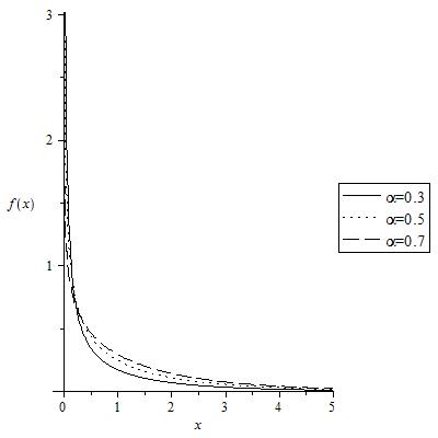 Figure 11
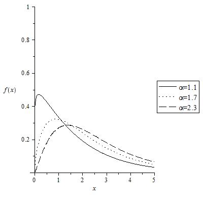 Figure 12
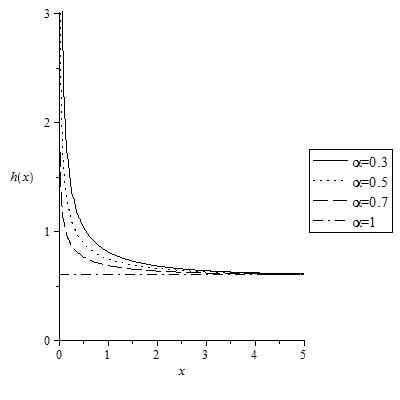 Figure 13
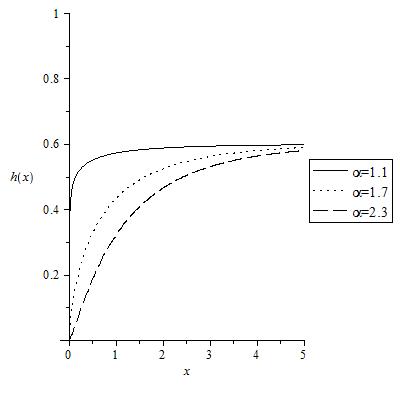 Figure 14
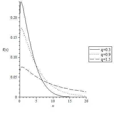 Figure 21
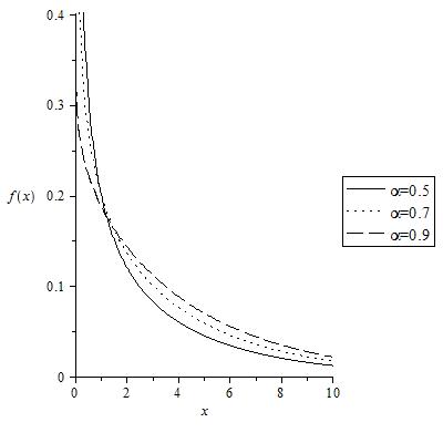 Figure 22
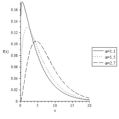 Figure 23
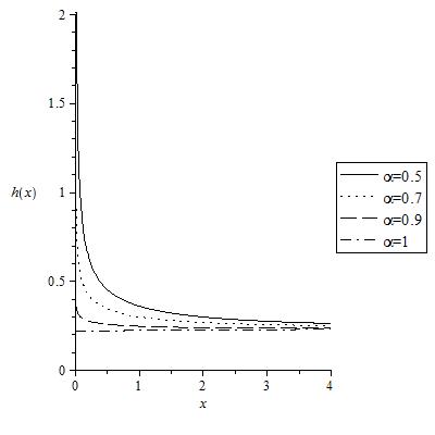 Figure 24
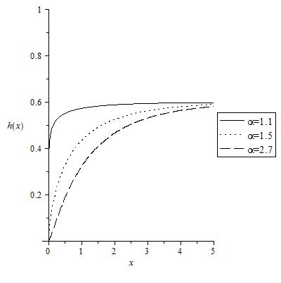 Figure 25
Peer Reviews
No public reviews on file for this paper yet. If you reviewed it on a platform where reviews are public (OpenReview, ICLR, NeurIPS, ICML), you can paste yours below so the community can read it here.
Videos
No videos yet. Explain this paper in a talk, walkthrough, or lecture? Add one.
Taxonomy
TopicsStatistical Distribution Estimation and Applications · Probability and Risk Models · Financial Risk and Volatility Modeling
**Topp-Leone generated q-exponential distribution and its applications **
Nicy Sebastian, Rasin R. S. and Silviya P. O.
Department of Statistics, St.Thomas College, Thrissur, Kerala, India-680001
e-mail: [email protected], [email protected]
Abstract
Topp-Leone distribution is a continuous model distribution used for modelling lifetime phenomena. The main purpose of this paper is to introduce a new framework for generating lifetime distributions, called the Topp-Leone generated q-exponential family of distributions. Parameter estimation using maximum likelihood method and simulation results to assess effectiveness of the distribution are discussed. Different informative and non-informative priors are used to estimate the shape parameter of q extended Topp-Leone generated exponential distribution under normal approximation technique. We prove empirically the importance and flexibility of the new model in model building by using a real data set.
Keywords: Topp-Leone distribution, beta-generated, generalized exponential, parameter estimation, simulation.
MSC (2010) 60E05, 33B20, 62G05, 62N05, 68U20.
1 Introduction
There are many statistical distributions which plays an important role in modeling survival and life time data such as exponential, weibull, logistic etc. Almost all these distributions with unbounded support. But there are situations in real life, in which observations can take values only in a limited range such as percentages, proportions or fractions. Papke and Wooldridge (1996) claims that in many economic settings, such as fraction of total weekly hours spent working, pension plan participation rates, industry market shares, fraction of land area allocated to agriculture etc., the variable bounded between zero and one. Thus it is important to have models defined on the unit interval in order to have reasonable results. Also different authors refer to continuous models with finite support in order to describe life time data, in reliability analysis. It is well known that beta distribution is the most used distribution to model continuous variables in the unit interval. This distribution is popular in the field of engineering, economics, biology, ecology etc. due to the great flexibility of its density function. But due to the fact that its distribution function cannot be expressed in closed form and it involves the incomplete beta function, the mathematical formulation is found to be difficult. However, several authors have proposed alternatives to the beta distribution by recovering the distribution proposed by Kumaraswamy in 1980.
A new distribution was introduced in 1955, called Topp Leone (TL) distribution, defined on finite support, proposed Topp and Leone and used it as a model for failure data. A random variable is distributed as the TL with parameter denoted by , with a cumulative distribution function
[TABLE]
The corresponding probability function is
[TABLE]
Topp Leone distribution provides closed forms of cumulative density function (cdf) and the probability density function (pdf) and describes empirical data with J-shaped histogram such as powered tool band failures, automatic calculating machine failure. The Topp Leone distribution had been received little attention until Nadarajah and Kotz (2003) discovered it. They studied about some properties of TL distribution and provided its moments, central moments and characteristic function. Ghitany et al. (2005) provided some reliability measures of TL distribution such as a hazard function, mean residual life, reversed hazard rate, expected inactivity time, an its stochastic orderings. A discussion on kurtosis of the TL distribution was reported by Kotz and Seier (2002).
Lifetime data plays an important role in a wide range of applications such as medical, engineering an social sciences. When there is a need for more flexible distributions, almost all researchers are about to use the new one with more generalization. An excellent review of Lee et al.(2013) has provided through knowledge of several methods for generating families of continuous univariate distributions. They classify these methods by years before and after 1980. According to their work, there are some general methods introduced prior to 1980, and they may be summarized as the method of differential equation, method of transformation (also known as translation), method of quantile. Since 1980, methodologies of generating new distribution shifted to adding new parameters to an existing distribution. According to Lee et al.(2013) some noticeable developments after 1980, are method of generating skew distributions, beta generated method, method of adding parameters, transformed-transformer method, and composite method.
The beta generated (BG) family of distributions belongs to a parameter adding mathod (Lee et al., (2013)). For an arbitrary distribution with a cumulative distribution function (cdf) and a probability density function (pdf) , this method generates it by letting where is the beta function, (see Alexander et al., 2012). Some existing distributions incorporated with BG family will have two additional parameters, which are the parameters of beta distribution. The cdf of beta generated random variable is defined as
[TABLE]
where is the pdf of beta random variable and is the cdf of any arbitrary random variable. Thus the cdf of beta generated random variable is
[TABLE]
The pdf corresponding to 3) is given by
[TABLE]
where is the beta function and is the gamma function.
Instead of using beta distribution as generator, we use TL distribution, as generator distribution, and we obtain TLG family of distribution. Then relation of a random variable having the TLG distribution and a random variable having TL distribution is with . This relation demonstrates that the pdf of TL distribution, (2), is transformed into a new pdf through the function
[TABLE]
By differentiating, we get the corresponding pdf,
[TABLE]
In reliability analysis, a frequently used distribution is exponential distribution having the characterizing property of constant hazard function. Due to this, exponential distribution is sometimes not suitable for analyzing data. This implies the need for more generalization. In such situations we use distribution called Topp-Leone Exponential distribution (TLE). TLE distribution comes as the combination of TL distribution and exponential distribution. Here TL distribution is the generator and exponential is the parent distribution. For creating TLE distribution, we need cdf G(x) and pdf g(x) of exponential distribution,
[TABLE]
and
[TABLE]
The TLE distribution is obtained by taking (7) and (8) into (5) and (6). Sangsanit and Bodhisuwan (2016) presented the Topp-Leone generated exponential (TLE) distribution as an example of the Topp-Leone generated distribution. A random variable possessing TLE distribution having cdf and probability function defined respectively as
[TABLE]
and
[TABLE]
Where is the shape parameter and is the scale parameter. The survival and hazard function of TLGE distribution is given as
and
.
respectively. It will be useful to consider the shape of the hazard function, in reliability analysis, to select appropriate distribution since it is an important measure of aging. For TLE distribution, depending on the values of the parameters, it can have constant, increasing, and decreasing hazard function. Plots of probability function and hazard function are respectively given in Figure 1 and Figure 2.
2 q-Exponential Distribution
Various entropy measures have been developed by mathematicians and physicists to describe several phenomena, depending on the field and the context in which it is being used. In statistical mechanics, Maxwell-Boltzmann distribution maximizes the Boltzmann-Gibbs entropy under appropriate constraints (Gell-Mann and Tsallis (2004)). Given a probability distribution with representing the probability of the system to be in the th microstate, the Boltzmann-Gibbs entropy is
[TABLE]
where is the Boltzmann constant and the total number of microstates. If all states are equally probable it leads to the Boltzmann principle . Boltzmann-Gibbs entropy is equivalent to Shannon’s entropy if . If we consider such a system in contact with a thermostat then we obtain the usual Maxwell-Boltzmann distribution for the possible states by maximizing the Boltzmann-Gibbs entropy with the normalization and energy constraints. However, in nature many systems show distributions which differ from the Maxwell-Boltzmann distribution. Tsallis (1988), introduced a generalization of the Boltzmann-Gibbs entropy. The -entropic function is of the form
[TABLE]
By maximizing Tsallis entropy, subject to certain constraints, leads to the Tsallis distribution, also known as -exponential distribution, which has the form where is the normalizing constant. Various applications and generalizations of the -exponential distribution are given in Picoli et al (2003). In the limit , -entropy converges to Boltzmann-Gibbs entropy.
An important characteristic of -exponential distribution is that it has two parameters and providing more flexibility with regard to its decay, differently from exponential distribution. The exponential distribution is defined by its pdf and cdf as,
[TABLE]
[TABLE]
The parameter is known as entropy index. As -exponential distribution becomes exponential distribution. In that sense -exponential distribution is a generalization of exponential distribution. The parameters and determine how quickly the pdf decays. In the reliability context, an important characteristic of the -exponential distribution is its hazard rate. It is given as
[TABLE]
For -exponential distribution, the hazard rate is not necessarily constant as in exponential distribution. For , is a decreasing monotonic function, while for , increases monotonically.
3 Topp-Leone q-Exponential Distribution
In this section we introduce the Topp-Leone generated q- exponential(TLqE) distribution by combining the TL distribution with q-exponential distribution. Substituting (10) and (11) in (5) and (6)respectively we will get the distribution function and density function of TLqE distribution as
[TABLE]
and
[TABLE]
In Figure 3 and Figure 4, we can see the plots of density function of TLqE for different values of the shape parameters and . The survival function, the probability density function and the Hazard function are the three important functions that characterize the distribution of the survival times. Here
,
and
respectively are the survival and the hazard function of TLqE distribution. Figure 5, gives the plots of of TLqE distribution for (left) and for (right) with . The cumulative hazard function is given as
[TABLE]
3.1 Maximum Likelihood Estimation
Here we derive the maximum likelihood estimate of the unknown parameter vector . Suppose be a random sample of size taken from TLqE distribution. We have the pdf of TLqE distribution is
[TABLE]
Then the likelihood function is written as
[TABLE]
and the log likelihood function is
[TABLE]
Let and . Thus can be written as
[TABLE]
Now differentiating with respect to and we get,
[TABLE]
Now setting , , and , and solving these system of equations simultaneously, we get the maximum likelihood estimate of . For solving these non-linear equations we can use any iteration method such as Newton-Raphson technique.
3.2 Bayesian Estimation
In this section our focus is to obtain the estimates of shape parameter of TLGqE distribution using Bayesian paradigm techniques by normal approximation. Large sample Bayesian methods are primarily based on normal approximation to the posterior distribution of . As the sample size increases, the posterior distribution approaches normality under certain regularity conditions and hence can be well approximated by an appropriate normal distribution if is sufficiently large. When is large, the posterior distribution becomes highly concentrated in a small neighborhood of the posterior mode, , for more details see Ghosh et al. (2006). If the posterior distribution is unimodal and roughly symmetric, it is convenient to approximate it by a normal distribution centered at the mode, and the logarithm of the posterior is approximated by a quadratic function, yielding the approximation
[TABLE]
If the mode, is in the interior parameter space, then is positive; if is a vector parameter, then is a matrix. The estimation of shape parameter of TL distribution using various Bayesian approximation techniques like normal approximation, Tierney and Kadane (T-K) Approximation are given by Sultan and Ahmad (2015).
In our study the normal approximations of Topp-Leone distribution under different priors is obtained as under: The likelihood function of (14) for a sample of size is given as
[TABLE]
where . Under uniform prior , the posterior distribution for is given as
[TABLE]
and
[TABLE]
where K is a constant. Then
[TABLE]
Hence the posterior mode is obtained as and . Thus, the posterior distribution can be approximated as
[TABLE]
Under extension of Jeffrey’s prior then the posterior distribution can be approximated as
[TABLE]
Under gamma prior then the posterior distribution can be approximated as
[TABLE]
3.3 Random Variate Generation
By using inversion method, we can generate a randon variate from TLqE distribution. We have already seen that the relationship between a random variable , having TLqE distribution, and a random variable , having the TL distribution, is
[TABLE]
where is related to inversion of the -exponential cdf. The quantile function of the TL distribution is
[TABLE]
where is picked from the uniform distribution over . Then the quantile function of TLqE distribution is obtained by substituting equation (17) into equation (16),
[TABLE]
For example, if =0.7235, 0.9690, 0.5374, 0.8221, 0.1961, then TLqE(0.3,1.5,1.2) can be generated respectively as
[TABLE]
Thus using this technique we can simulate random variates for any values of the parameters.
3.4 Application
In this section, we consider a real data set and try to find the distribution that fits better to the data among the TLqE distrubution and TLE distribution. For the purpose of model selection, we use the Akaike Information Criterion (AIC), and the Bayesian Information criterion (BIC). The real data set that we consider, is the ball bearing data, which says the number of revolutions before failure for ball bearing (Crowder et al.,1994).
The data is 33.00, 68.64, 173.40, 41.52, 42.12, 68.64, 68.88, 45.60, 48.48, 84.12, 93.12, 98.64, 105.12, 105.84, 51.84, 51.96, 54.12, 17.88, 55.56, 127.92, 128.04, 67.80, 67.80, 28.92. We provide the values of estimated parameters, AIC and BIC values for ball bearing data in the table given below.
[TABLE]
The AIC and BIC values of the TLqE distribution is the smallest ones among the three considered distributions. As expected TLqE is more appropriate for this data than the TLE distribution because of its shape of hazard function.
The reference list from the paper itself. Each links out to its DOI / PubMed record.
- 1[1] Alexander, C., Cordeiro, G.M., Ortega and Sarabia,J. M. (2012). Generalized beta generated distribution. Computational Statistics and the Data Analysis 56,1880- 1897.
- 2[2] Alzaatreh, A.,Lee, C.and Famoye,F. (2013). A new method for generating families of continuous distributions. METRON 71, 63-79.
- 3[3] Crowder, M. J., Kimber, A. C., Smith, R. L. and Sweeting, T. J. (1991). Statistical Analysis of Reliability Data. New York, NY: Chapman and Hall.
- 4[4] Gell-Mann, M. and Tsallis C. (Eds.). (2004). Nonextensive Entropy: Interdisciplinary Applications. Oxford University Press, New York,
- 5[5] Ghitany M. E. , Kotz S. And Xie, M. (2005) .On some reliability measures and their stochastic orderings for the Topp-Leone distribution, Journal of Applied Statistics, 32(7), 715-722.
- 6[6] Ghosh, J. K., Delampady, M. and Samanta, T. (2006). An Introduction to Bayesian Analysis Theory and Methods, Springer-Verlag New York.
- 7[7] Kotz, S. and Seier, E. (2007). Kurtosis of the Topp-Leone distributions. Interstat, 2007 (July).
- 8[8] Lee, C.,Famoye,F. and Alzaatreh, A.Y.(2013). Methods of generating families of univariate continuous distributions in the recent decades. WIR Es Comput Stat 5, 219-238.