This paper develops rate-optimal, robust nonparametric estimators for the leading coefficient of linear SPDEs using localized continuous observations, with theoretical analysis and numerical validation.
Contribution
It introduces new nonparametric estimation methods for linear SPDEs from local measurements, achieving parametric rates and robustness to perturbations.
Findings
01
Establishes asymptotic properties of estimators in fixed time and shrinking spatial resolution regimes.
02
Provides scaling limits of the PDE and SPDE on expanding domains.
03
Demonstrates estimator robustness to lower order operator perturbations.
Abstract
The coefficient function of the leading differential operator is estimated from observations of a linear stochastic partial differential equation (SPDE). The estimation is based on continuous time observations which are localised in space. For the asymptotic regime with fixed time horizon and with the spatial resolution of the observations tending to zero, we provide rate-optimal estimators and establish scaling limits of the deterministic PDE and of the SPDE on growing domains. The estimators are robust to lower order perturbations of the underlying differential operator and achieve the parametric rate even in the nonparametric setup with a spatially varying coefficient. A numerical example illustrates the main results.
No public reviews on file for this paper yet. If you reviewed it on a platform where reviews are public (OpenReview, ICLR, NeurIPS, ICML), you can paste yours below so the community can read it here.
Videos
No videos yet. Explain this paper in a talk, walkthrough, or lecture? Add one.
Full text
Nonparametric estimation for linear SPDEs
from local measurements
Randolf Altmeyer, Markus Reiß
Humboldt-Universität zu Berlin 111Institut für Mathematik, Humboldt-Universität zu Berlin, Unter den Linden 6, 10099 Berlin, Germany. Email: [email protected], [email protected].
We are grateful to Sylvie Roelly, Nicolas Perkowski, Josef Janák and two anonymous referees for very helpful comments and questions.
This research has been partially funded by Deutsche Forschungsgemeinschaft (DFG) - SFB1294/1 - 318763901.
*
Abstract
The coefficient function of the leading differential operator is estimated from observations of a linear stochastic partial differential equation (SPDE). The estimation is based on continuous time observations which are localised in space. For the asymptotic regime with fixed time horizon and with the spatial resolution of the observations tending to zero, we provide rate-optimal estimators and establish scaling limits of the deterministic PDE and of the SPDE on growing domains. The estimators are robust to lower order perturbations of the underlying differential operator and achieve the parametric rate even in the nonparametric setup with a spatially varying coefficient. A numerical example illustrates the main results.
While there is a large amount of work on probabilistic, analytical
and recently also computational aspects of stochastic partial differential
equations (SPDEs), many natural statistical questions are open. With
this work we want to enlarge the scope of statistical methodology
in two major directions. First, we consider observations of a solution
path that are local in space and we ask whether the underlying differential
operator or rather its local characteristics can be estimated from
this local information only. Second, we allow the coefficients in
the differential operator to vary in space and we pursue nonparametric
estimation of the coefficient functions, as opposed to parametric
estimation approaches for finite-dimensional global parameters in
the coefficients. Naturally, both directions are intimately connected.
As a concrete model we consider the parabolic SPDE
[TABLE]
with the second-order differential operator Aϑz:=div(ϑ∇z)+⟨a,∇z⟩+bz
on some bounded domain Λ⊆Rd with Dirichlet boundary conditions, see Section 2
for formal details. The coefficient functions ϑ,a,b are unknown
on Λ and we aim at estimating ϑ:Λ→R+,
which models the diffusivity in a stochastic heat equation. The functions
a,b as well as the operator B in front of the driving space-time
white noise process dW form an unknown nuisance part. Linear SPDEs of this form appear in many applications, including neuroscience (Walsh, [38]), oceanography (Frankignoul, [14]), geostatistics (Sigrist et al., [36]), surface growth (Edwards & Wilkinson, [10]) and finance (Cont, [8]).
Measurements of a solution process X necessarily have a minimal
spatial resolution δ>0 and we dispose of the observations
⟨X(t),Kδ,x0⟩, where the solution is integrated in the spatial domain against
a kernel function Kδ,x0 with support of diameter
δ around some x0∈Λ. We keep the time span T
fixed and construct an estimator, called proxy MLE, which
for the resolution asymptotics δ→0 converges at rate δ
to ϑ(x0) and satisfies a CLT, which we derive in the case of a local multiplication covariance operator B in the SPDE. Another estimator, the so-called
augmented MLE, will even converge under far more general
conditions and exhibit a smaller asymptotic variance, but requires
a second local observation process ⟨X(t),ΔKδ,x0⟩
in terms
of the Laplace operator Δ. Clearly, if we have access to these
observations around all x0∈Λ, then both estimators can
be used to estimate the diffusivity function ϑ nonparametrically
on all of Λ.
These results are statistically remarkable. First of all, even for
the parametric case that ϑ is a constant, it is not immediately
clear that ϑ is identified (i.e., exactly recovered) from
local observations in a shrinking neighbourhood around some x0∈Λ
only. Probabilistically, this means that the local observation laws
are mutually singular for different values of ϑ. What is more,
the bias-variance trade-off paradigm in nonparametric statistics does
not apply: asymptotic bias and standard deviation are both of order
δ and the CLT provides us even with a simple pointwise confidence
interval for ϑ. The robustness of the estimators to lower
order parts in the differential operator and unknown B is very
attractive for applications. The rate δ is shown to be the
best achievable rate in a minimax sense even for constant ϑ
without nuisance parts.
The fundamental probabilistic structure behind these results is a
universal scaling limit of the observation process for δ→0.
At a highly localised level, the differential operator Aϑ
behaves like ϑ(x0)Δ, as expressed in Corollary 3.6
below, and the construction of the estimators shows a certain scaling
invariance with respect to B. To study these scaling limits, we
need to consider the deterministic PDE on growing domains via the
stochastic Feynman-Kac approach and to deduce tight asymptotics for
the action of the semigroup and the heat kernels. Further tools like
the fourth moment theorem or the Feldman-Hajek Theorem rely on the
underlying Gaussian structure, but extensions to semi-linear SPDEs
seem possible.
Let us compare our localisation approach to the spectral approach,
introduced by Huebner et al., [18] and then in Huebner & Rozovskii, [20] for parametric estimation. In
the simplest case Aϑ=ϑΔ for some ϑ>0
and B commuting with Aϑ, the SPDE solution can be expressed
in the eigenbasis of the Laplace operator Δ. If the first
N coefficient processes (Fourier modes of X) are observed, then
a maximum-likelihood estimator for ϑ is asymptotically efficient
as N→∞. This approach has turned out to be very versatile,
allowing also for estimating time-dependent ϑ(t) nonparametrically
(Huebner & Lototsky, [19]) or to cover nonlinear SPDEs (Cialenco & Glatt-Holtz, [6],
Pasemann & Stannat, [31]). In particular, it helps to understand that the coefficient in the leading order of the differential operator
can be estimated with better rates than lower order coefficients. The methodology, however, is intrinsically
bound to observations in the spectral domain and to operators Aϑ
whose eigenfunctions, at least in the leading order, are independent
of ϑ. In contrast, we work with local observations in space
and the unknown spectrum of the operators Aϑ does not harm
us. More conceptually, we rely on the local action of the differential
operator Aϑ, while the spectral approach also applies to
an abstract operator in a Hilbert space setting.
Our case of spatially varying coefficients has been considered first
by Aihara & Sunahara, [3] (with a=b=0) in a filtering problem.
The corresponding nonparametric estimation problem is then addressed
by Aihara & Bagchi, [2] with a sieve least squares estimator, but
they achieve consistency only for global observations with a growing
time horizon T→∞. In a stationary one-dimensional setting
Bibinger & Trabs, [4] ask whether the parameter ϑ>0 can be
estimated when observing the solution only at x0 over a fixed
time interval [0,T]. Interestingly, in the case B=σ2I
the parameter ϑ cannot be recovered if the level σ
of the space-time white noise is unknown (see also lower bounds of Hildebrandt & Trabs, [17]). For a recent and exhaustive
survey on statistics for SPDEs we refer to Cialenco, [5].
In Section 2 the SPDE and the observation model are introduced
and in Section 3 the scaling properties along with the
resolution level δ are discussed. Section 4
derives our estimators via a least-squares and a likelihood approach
and provides basic insight into their error analysis. The main
convergence results as well as a minimax lower bound are presented
in Section 5. The findings are illustrated by
a numerical example in Section 6.
While the main steps in the proofs are presented together with the
results, all more technical arguments are delegated to the Appendix.
2 The model
2.1 Notation
Let Λ be a bounded open set in Rd with C2-boundary
∂Λ and consider L2(Λ) with the usual L2-norm
∥⋅∥:=∥⋅∥L2(Λ). For any open set U in Rd and any linear operator A:L2(U)→L2(U) let ∥A∥L2(U):=∥A∥L2(U)→L2(U) denote the operator norm, and let Hk(U) for k∈N be the L2-Sobolev spaces. Define H01(Λ) as the closure of Cc∞(Λ) in H1(Λ). We write ⟨⋅,⋅⟩Rd
for the Euclidean inner product and ∣⋅∣ for the norm. Let us define a second order elliptic operator with
Dirichlet boundary conditions
[TABLE]
where Δϑz=div(ϑ∇z)=∑i=1d∂i(ϑ∂iz)
is the weighted Laplace operator with spatially varying diffusivity
ϑ∈C1+α(Λ) for α>0, minx∈Λϑ(x)>0, and where A0z=⟨a,∇z⟩Rd+bz with functions a∈C1+α(Λ;Rd),
b∈Cα(Λ). The
regularity conditions on ϑ,a,b are such that the deterministic
PDE dtdu(t)=Aϑ∗u(t) with initial value z∈L2(Λ)
has a sufficiently smooth solution (see proof of Proposition 3.5
below). Let (Sϑ(t))t⩾0 denote the analytic semigroup on L2(Λ) generated by Aϑ (cf. Theorem 3.1.3 of Lunardi, [28]), while (etΔ)t⩾0 is the heat semigroup on L2(Rd) generated
by Δ=Δ1 with domain H2(Rd).
2.2 The SPDE model
Throughout this work T<∞ is fixed. Let (Ω,F,(Ft)0⩽t⩽T,P)
be a filtered probability space with a cylindrical Brownian motion
W on L2(Λ) (dW is also referred to as space-time
white noise), and let B:L2(Λ)→L2(Λ)
be a bounded linear operator, which is not assumed to be trace class.
We study the linear stochastic partial differential equation
[TABLE]
with deterministic initial value X0∈L2(Λ).
Our statistical analysis below relies on linear functionals of X(t)
rather than on X(t) itself. We therefore use the weak solution
concept of Da Prato & Zabczyk, [9]. If ∫0T∥Sϑ(t)B∥HS(L2(Λ))2dt<∞
with Hilbert-Schmidt norm ∥⋅∥HS(L2(Λ)), then
the unique weak solution (X(t))0⩽t⩽T of the SPDE (2.1)
is given by the variation of constants formula, cf. Theorem 5.4 of
Da Prato & Zabczyk, [9],
[TABLE]
It takes values in L2(Λ) and satisfies for z∈H01(Λ)∩H2(Λ)
[TABLE]
Clearly, for z∈L2(Λ)
[TABLE]
If ∫0T∥Sϑ(t)B∥HS(L2(Λ))2dt=∞,
then the stochastic integral in (2.2) is well-defined
only in a space of distributions. For example, if H−s(Λ) is a fractional Sobolev space of negative order with s>d/4, then the natural
embedding ι:L2(Λ)→H−s(Λ) is a
Hilbert-Schmidt operator such that ∫0T∥ιSϑ(t)B∥HS(L2(Λ),H−s(Λ))2dt<∞,
and X(t) takes values in H−s(Λ) (cf. Remark 5.6 of
Hairer, [16]). Still, (2.3) and (2.4)
remain valid, if ⟨X(t),z⟩ and ⟨X(t),Aϑ∗z⟩ are
interpreted as dual pairings between H−s(Λ) and its dual space
for z∈Cc∞(Λ).
On the other hand, denote the right hand side of the equation in (2.4)
by ℓ(t,z) and observe that it is always well-defined for any z∈L2(Λ),
independent of the space in which (2.2) makes
sense, cf. Lemma 2.4.2 of Liu & Röckner, [26]. The resulting process ℓ:=(ℓ(t,z))0⩽t⩽T,z∈L2(Λ)
thus extends the linear forms z↦⟨X(t),z⟩ from Cc∞(Λ) to L2(Λ). It has the following properties.
2.1 Proposition**.**
ℓ* is a Gaussian process with
mean function (t,z)↦⟨Sϑ(t)X0,z⟩
and covariance function at 0⩽t,t′⩽T, z,z′∈L2(Λ)
given by*
[TABLE]
Moreover, ℓ satisfies (2.3) for z∈H01(Λ)∩H2(Λ),
if ⟨X(t),z⟩ and ⟨X(t),Aϑ∗z⟩ are replaced by
ℓ(t,z) and ℓ(t,Aϑ∗z).
Proof.
By (2.4), ℓ(t,z) for z∈L2(Λ)
is Gaussian with mean ⟨Sϑ(t)X0,z⟩.
Itô’s isometry (Proposition 4.28 of Da Prato & Zabczyk, [9]) proves
(2.5). If z∈Cc∞(Λ),
then ℓ(t,z)=⟨X(t),z⟩ satisfies dℓ(t,z)=ℓ(t,Aϑ∗z)dt+d⟨BW(t),z⟩. This
extends to z∈H01(Λ)∩H2(Λ) by approximation
and continuity of ℓ:[0,T]×L2(Λ)↦L2(P)
from (2.5).
∎
In the following, justified by this proposition, we write ⟨X(t),z⟩
for 0⩽t⩽T and z∈L2(Λ) instead of ℓ(t,z).
2.3 Local observations
Throughout this work let x0∈Λ be fixed. The following
rescaling will be useful in the sequel: for z∈L2(Rd)
and δ>0 set
[TABLE]
Fix a function
K∈H2(Rd), called kernel, with compact support in Λδ,x0.
The compact support ensures that Kδ,x0 is localized
around x0 and Kδ,x0∈H01(Λ)∩H2(Λ),
∥Kδ,x0∥=∥K∥L2(Rd). Local measurements
of X at x0 with resolution level δ until time T
are described by the real-valued processes Xδ,x0=(Xδ,x0(t))0⩽t⩽T,
Xδ,x0Δ=(Xδ,x0Δ(t))0⩽t⩽T,
[TABLE]
Note that it is sufficient to observe Xδ,x(t) for x
in a neighbourhood of x0 in order to provide us with Xδ,x0Δ(t)=ΔXδ,⋅(t)∣x=x0.
Examples for K can be found in Section 6.
The process Xδ,x0 satisfies Xδ,x0(0)=⟨X0,Kδ,x0⟩
and
[TABLE]
with the scalar Brownian motion W(t)=⟨BW(t),Kδ,x0⟩/∥B∗Kδ,x0∥,
whenever ∥B∗Kδ,x0∥>0.
3 Scaling assumptions
3.1 Rescaled operators and semigroups
Let us study how Aϑ∗ and Sϑ∗(t)
act on localized functions zδ,x0. For this note first
that Aϑ∗=Δϑ+A0∗ with A0∗z=−div(az)+bz
has domain D(Aϑ∗)=H01(Λ)∩H2(Λ).
For δ>0 define similarly the operator Aϑ,δ,x0∗=Δϑ(x0+δ⋅)+A0,δ,x0∗
with domain D(Aϑ,δ,x0∗)=H01(Λδ,x0)∩H2(Λδ,x0),
where for z∈Cc∞(Λδ,x0)
[TABLE]
The operator Aϑ,δ,x0∗
generates again an analytic semigroup (Sϑ,δ,x0∗(t))t⩾0 on L2(Λδ,x0) (Lemma 7.3.4 of Pazy, [32]). The following scaling properties are fundamental for our analysis:
3.1 Lemma**.**
For δ>0:
(i)
If z∈H01(Λδ,x0)∩H2(Λδ,x0),
then Aϑ∗zδ,x0=δ−2(Aϑ,δ,x0∗z)δ,x0.
2. (ii)
If z∈L2(Λδ,x0), then Sϑ∗(t)zδ,x0=(Sϑ,δ,x0∗(tδ−2)z)δ,x0,
t⩾0.
Proof.
It suffices to prove the result for z∈Cc∞(Λδ,x0). In this case, (i) follows immediately, noting that zδ,x0∈Cc∞(Λ). For (ii) set w(t)=(Sϑ,δ,x0∗(tδ−2)z)δ,x0∈L2(Λ).
As (Sϑ,δ,x0∗(t))t⩾0 is an analytic semigroup,
we have Sϑ,δ,x0∗(t)z∈D(Aϑ,δ,x0∗)=H01(Λδ,x0)∩H2(Λδ,x0)
and so by (i)
[TABLE]
Since w(0)=zδ,x0, we conclude that w(t)=Sϑ∗(t)zδ,x0 from u(t)=Sϑ∗(t)zδ,x0
being the unique solution in C([0,∞);H01(Λ)∩H2(Λ))∩C1([0,∞);L2(Λ))
of
[TABLE]
Applying Sϑ∗(t) to a localized function zδ,x0
is therefore equivalent to applying a different semigroup, rescaled
in time and space, to the fixed function z.
3.2 Scaling of B
Just as with Aϑ∗ we also need that B∗ behaves
nicely when applied to localized functions. For this we shall assume
a scaling limit for B∗, which does not degenerate in combination
with K.
3.2 Assumption**.**
There are bounded linear operators
Bδ,x0,B0,x0:L2(Rd)→L2(Rd)
such that B∗(zδ,x0)=(Bδ,x0∗z)δ,x0
for z∈L2(Rd) with support in Λδ,x0
and Bδ,x0∗z→B0,x0∗z for z∈L2(Rd)
and δ→0. Introducing
[TABLE]
assume the non-degeneracy conditions∥B0,x0∗K∥L2(Rd)>0,
Ψ(ΔK,ΔK)>0.
3.3 Remark**.**
We shall see that after an appropriate rescaling
ϑ(x0)−1Ψ(z,z′) becomes the limiting covariance in
(2.5) (cf. Proposition A.8 below).
Ψ(ΔK,ΔK) is always nonnegative and finite because
[TABLE]
using ∥esΔΔK∥L2(Rd)2=⟨e2sΔΔK,ΔK⟩L2(Rd)
and ∫0∞e2sΔΔKds=−21K.
3.4 Examples**.**
(a)
For a bounded continuous function σ:Rd→(0,∞) define
the multiplication operator Mσ:L2(Λ)→L2(Λ),
Mσz(x):=(σz)(x)=σ(x)z(x). With B=B∗=Mσ
the SPDE in (2.1) can be written informally as
[TABLE]
Note that B∗ commutes with Aϑ only if σ is constant.
For z∈L2(Λδ,x0) we find that B∗zδ,x0=(Mσ(δ⋅+x0)z)δ,x0
and so Bδ,x0=Mσ(δ⋅+x0). Then ∥Bδ,x0∗z−σ(x0)z∥L2(Rd)→0
for z∈L2(Rd), δ→0, and thus B0,x0∗=Mσ(x0)
is the multiplication operator on L2(Rd) with the constant
σ(x0). For z∈H2(Rd), z′∈L2(Rd)
we have (cf. Remark 3.3)
[TABLE]
and integration by parts shows Ψ(ΔK,ΔK)=2σ2(x0)∥∇K∥L2(Rd)2.
The non-degeneracy conditions are clearly satisfied.
2. (b)
Let σ be as in (a) and consider with bounded η∈C2(Rd),
minx∈Rdη(x)>0, the perturbed multiplication operator
B=B∗=Mσ+(−Δη)−γ, γ>0. By
functional calculus B∗zδ,x0=(Bδ,x0∗z)δ,x0
for z∈L2(Λδ,x0) with Bδ,x0=Mσ(δ⋅+x0)+δ2γ(−Δη(δ⋅+x0))−γ
and ∥Bδ,x0∗z−σ(x0)z∥L2(Rd)→0
for z∈L2(Rd), δ→0. B0,x0 and
Ψ(ΔK,ΔK) are as in (a).
3. (c)
Assumption 3.2 excludes B=(−Δ)−γ, γ>0,
a typical choice to obtain smooth solutions X, cf. Da Prato & Zabczyk, [9, Chapter 5.5].
Indeed, by (b) Bδ,x0∗=δ2γ(−Δ)−γ
and so B0,x0∗=0, violating the non-degeneracy conditions.
This problem can be solved by modifying the test function Kδ,x0.
For example, if Aϑ=ϑΔ for constant ϑ>0
and X0∈D((−Δ)γ), then assume we have access to ⟨X(t),(−Δ)γKδ,x0⟩,
⟨X(t),(−Δ)γΔKδ,x0⟩ instead of (2.6),
(2.7). Since B and Aϑ commute, ⟨X(⋅),(−Δ)γKδ,x0⟩
has the same distribution as ⟨X~(⋅),Kδ,x0⟩,
where X~ corresponds to the SPDE (2.1) with B=I
and X~0=(−Δ)γX0, and so Assumption 3.2
is satisfied.
3.3 From bounded to unbounded domains
Lemma 3.1 and Assumption 3.2 allow us to
rewrite the covariance function of Xδ,x0 for t,t′⩾0:
[TABLE]
In order to see how this behaves when δ→0, note that the domain Λδ,x0 grows
and we find from (3.1) that Aϑ,δ,x0∗K→ϑ(x0)ΔK
in L2(Rd). This motivates the following result, proved in Appendix A.2.
3.5 Proposition**.**
For t>0:
(i)
If δ>0 and z∈C(Λδ,x0), then
∣(Sϑ,δ,x0∗(t)z)(x)∣⩽c3ec1δ2t(ec2tΔ∣z∣)(x)
for all x∈Λδ,x0 with universal constants c1,c2,c3>0.
2. (ii)
If z∈L2(Rd), then Sϑ,δ,x0∗(t)(z∣Λδ,x0)→eϑ(x0)tΔz
in L2(Rd) for δ→0.
This means that the solution of
[TABLE]
on L2(Λδ,x0) with bounded domainΛδ,x0
converges to the solution of the heat equation
[TABLE]
on L2(Rd) with unbounded domainRd. This
scaling limit,
which seems natural but is nevertheless non-trivial, lies at the heart
of the analysis for the covariance function. Yet, the convergence in Proposition 3.5(ii)
does not hold uniformly in z, which complicates the approximations in the covariance analysis.
Applying the proposition to (3.4) also implies a scaling limit for the SPDE in (2.1),
where for simplicity a zero initial condition is assumed:
3.6 Theorem**.**
Let X0=0 and set Zδ(t,z):=δ−1⟨X(tδ2),(z∣Λδ,x0)δ,x0⟩
for t⩾0, z∈L2(Rd). Under Assumption 3.2
the finite dimensional distributions of (Zδ(t,z))t⩾0,z∈L2(Rd)
converge to those of (Z0(t,z))t⩾0,z∈L2(Rd),
Z0(t,z)=⟨Y(t),z⟩L2(Rd), solving the stochastic heat
equation on L2(Rd) with space-time white noise dW on L2(Rd):
[TABLE]
Proof.
According to (3.4) Zδ
is a centered Gaussian process with covariance function Cov(Zδ(t,z),Zδ(t′,z′))
for t,t′⩾0, z,z′∈L2(Rd) equal to
[TABLE]
It is enough to show that this converges to
[TABLE]
Approximating z by continuous functions, the semigroup bound in Proposition 3.5(i)
gives sup0<δ⩽1sups⩽t∥Sϑ,δ,x0∗(s)(z∣Λδ,x0)∥L2(Λδ,x0)<∞,
while Assumption 3.2 implies Bδ,x0∗u(δ)→B0,x0∗u for any u(δ)→u, invoking the uniform boundedness principle.
By Proposition 3.5(ii)
we have Sϑ,δ,x0∗(s)(z∣Λδ,x0)→eϑ(x0)sΔz
in L2(Rd). Arguing in the same way with respect to z′, the dominated
convergence theorem shows the claim.
∎
This theorem demonstrates the strength of local measurements that
at small scales the highest order differential operator dominates,
together with the local coefficient ϑ(x0) and the local
operator B0,x0 in the noise.
3.4 The initial condition
For X0 we require the following scaling behaviour:
3.7(z;β) Assumption****.
For β>0
and z∈H2(Rd) with compact support in Λδ,x0
for δ>0, the initial condition X0 satisfies
[TABLE]
where ℓd,2(δ)=log(δ−1) for d=2 and ℓd,2(δ)=1
otherwise.
Under this assumption the initial condition becomes negligible in the estimation procedure. It is true under general conditions.
3.8 Lemma**.**
Assumption 3.7(z;β) Assumption(z;β)
is satisfied for all z∈H2(Rd) with compact support in
Λδ,x0 for δ>0 and
(i)
β=2* if X0∈Lp(Λ) for some p>2, in particular
if X0∈C(Λ),*
2. (ii)
β=3* if X0∈D(Aϑ).*
Proof.
This follows from Lemma A.7(ii,iii) below, noting γ(d,p)>2 in (ii) for p>2, d⩾1.
∎
4 The two estimation methods
4.1 Motivation and construction
We give two motivations for deriving the estimators in the parametric
case Aϑ=ϑΔ with constant ϑ>0, B=I.
As we shall see later, these estimators will then work quite universally
for nonparametric specifications of ϑ and general Aϑ
and B.
Least squares approach.
In the deterministic situation of (2.8) without driving
noise (i.e. Aϑ=ϑΔ and B=0) we recover ϑ
via X˙δ,x0(t)=ϑXδ,x0Δ(t)
for all t∈[0,T]. A standard least-squares ansatz in the noisy
situation would therefore lead to an estimator ϑ^=argminϑ∫0T(X˙δ,x0(t)−ϑXδ,x0Δ(t))2dt.
While this itself is certainly not well defined, the corresponding
normal equations yield the feasible estimator
[TABLE]
compare with the approach by Maslowski & Tudor, [29] for fractional
noise.
Likelihood approach.
Assume that only Xδ,x0 in (2.8) is observed with Aϑ=ϑΔ, B=I. Denote by Pϑδ,x0 and
P0 the laws of Xδ,x0 and ∥K∥L2(Rd)W
on the canonical path space (C([0,T]),∥⋅∥∞)
equipped with its Borel sigma algebra. Typically, the likelihood of
Pϑδ,x0 with respect to P0 is determined
via Girsanov’s theorem. This is not immediate from (2.8),
because Xδ,x0Δ cannot be obtained from Xδ,x0
for fixed x0. Therefore we employ Liptser & Shiryaev, [25, Theorem 7.17]
and write Xδ,x0 as the diffusion-type process
[TABLE]
with a different scalar Brownian motion W~=(W~(t))0⩽t⩽T,
adapted to the filtration generated by Xδ,x0, and
[TABLE]
Girsanov’s theorem in the form of Liptser & Shiryaev, [25, Theorem 7.18]
applies and we find that Pϑδ,x0 has with respect
to P0 the likelihood
[TABLE]
Computing the conditional expectation mϑ(t) is a non-explicit
filtering problem, even in the parametric case Aϑ=ϑΔ.
In particular, mϑ depends on ϑ in a highly nonlinear
way. We pursue two different modifications:
Augmented MLE.
If we observe Xδ,x0Δ additionally, then we can
just replace the conditional expectation mϑ(t) in the likelihood
by its argument Xδ,x0Δ(t), which is in particular
independent of ϑ. Maximizing this modified likelihood leads
to the augmented MLE
[TABLE]
We remark that ϑ^δA=ϑ^δLS.
Proxy MLE.
If we do not dispose of additional observations, we can approximate
mϑ(t) by the conditional expectation Eϑ[Xδ,x0Δ(t)∣Xδ,x0(t)].
In our simplified setup with Aϑ=ϑΔ and B=I
the projected finite-dimensional process (⟨X(t),zi⟩)1⩽i⩽m for zi∈L2(Λ) admits a stationary solution
⟨X(t),zi⟩=∫−∞t⟨Sϑ(t−s)zi,dW(s)⟩, i=1,…,m,
with a two-sided cylindrical Brownian motion (W(t))t∈R, provided
the variances remain finite. Note that we need not require X0=∫−∞tSϑ∗(t−s)dW(s) to exist, but only that the finite-dimensional projection (⟨X0,zi⟩)1⩽i⩽m follows the right law, which is always feasible. If we choose z1=Kδ,x0, z2=ΔKδ,x0, then the process (Xδ,x0,Xδ,x0Δ) is stationary with
[TABLE]
In general, ⟨(−Δ)−1Kδ,x0,Kδ,x0⟩
may not exist, but if we assume the existence of K~∈H4(Rd)
with ΔK~=K and compact support in Λδ,x0,
then by the scaling in Lemma 3.1, Var(Xδ,x0(t))=2ϑδ2∥∇K~∥L2(Rd)2<∞
follows. In this situation we therefore find that Eϑ[Xδ,x0Δ(t)∣Xδ,x0(t)]
equals
[TABLE]
This expression is again independent of ϑ. Using it as an
approximation of mϑ(t) in the likelihood and neglecting
the boundary terms in the identity 2∫0TXδ,x0(t)dXδ,x0(t)=(Xδ,x02(T)−Xδ,x02(0))−⟨Xδ,x0⟩T
with quadratic variation ⟨Xδ,x0⟩T, we
obtain the proxy MLE
[TABLE]
Note that the quadratic variation ⟨Xδ,x0⟩T=T∥B∗Kδ,x0∥2
is known to us from observing Xδ,x0 continuously in
time.
4.1 Remark**.**
A sufficient condition for the existence of K~ is ∫RdK(x)dx=0,
∫RdxK(x)dx=0 by Lemma A.5(iii) below.
4.2 Basic error decomposition
Let us discuss the basic error analysis for the augmented MLE ϑ^δA
and the proxy MLE ϑ^δP in the general nonparametric
framework of Section 2. Since we only use local measurements
around x0, it might be expected that asymptotically we are lead to estimating
ϑ(x0). Let us point out that this is indeed true, but a priori not clear because all values of ϑ(x) enter into the observations Xδ,x0 and it must be excluded that the resulting bias spoils the estimator.
Augmented MLE.
Consider ϑ^δA(x0)=ϑ^δA
from (4.1). Then insertion of Equation (2.8)
for dXδ,x0(t) yields the decomposition
[TABLE]
with
[TABLE]
Let us note that IδA is not the observed Fisher information
in a strict sense (due to the appearance of mϑ in the likelihood),
but it plays the same role, compare the analysis of the MLE for Ornstein-Uhlenbeck
processes in Kutoyants, [24]. In particular, it
forms the quadratic variation of the martingale MδA.
In the specific case Aϑ=ϑΔ for some parametric
ϑ>0 the term RδA vanishes, otherwise it induces
a bias due to the variations of ϑ around ϑ(x0)
and due to first and zero order differential operators that may appear
in Aϑ.
As the error structure suggests, the augmented MLE ϑ^δA(x0)
is a consistent estimator for δ→0 if the observed Fisher
information satisfies IδA→∞. In the simple
stationary case of (4.2) we obtain E[IδA]=2ϑT⟨(−Δ)Kδ,x0,Kδ,x0⟩,
which by the scaling properties is of order δ−2. Physically,
this can be interpreted as an increase in energy in Xδ,x0Δ
under δ-localisation due to the Laplacian in the drift, while
the energy from the space-time white noise remains unchanged. This
is in fact the same phenomenon as the increasing signal-to-noise ratio
for high Fourier modes in the spectral approach by Huebner & Rozovskii, [20].
Proxy MLE.
Consider ϑ^δP(x0)=ϑ^δP
from (4.3). The only stochastic part is
[TABLE]
in the denominator. In the general model (2.8) we
shall see that IδP converges to ϑ(x0)−1TΨ(K,K),
compare also Remark 3.3 with K=ΔK~. Asking
for consistency ϑ^δP(x0)→ϑ(x0)
leads to requiring the identity ∥∇K~∥L2(Rd)2∥B0,x0∗K∥L2(Rd)2=2∥K∥L2(Rd)2Ψ(K,K).
This does not hold for any operator B0,x0. We therefore restrict
to our main specification B=Mσ, for which the identity
holds by (3.3). In contrast to the augmented
MLE, the proxy MLE works with the observation of Xδ,x0
alone, but asks for new structural assumptions on B and K. If
they are not fulfilled, other likelihood approximations should be
pursued. Compare also the suboptimal behaviour of ϑ^δP(x0)
for the kernel K(2) in the simulations of Section 6
below.
5 Main results
5.1 Results for the augmented MLE
Recall the function Ψ from (3.2) and
the error decomposition (4.4). We show first that
the observed Fisher information and the bias, after rescaling, converge
to deterministic quantities. The propositions are proved in Appendix A.1.
In terms of Yt(δ):=Xδ,x0Δ(t)/E[IδA]1/2
we obtain MδA/E[IδA]1/2=∫0TYt(δ)dWˉ(t),
the quadratic variation of which satisfies ∫0T(Yt(δ))2dt=IδA/E[IδA]P1
by Proposition 5.1. A standard continuous
martingale CLT, e.g. Kutoyants, [24, Theorem 1.19],
shows MδA/E[IδA]1/2dN(0,1).
Moreover,
[TABLE]
due to Assumption 3.2 and δ−1(IδA)−1RδAPμA
by Proposition 5.2. We conclude by applying
Slutsky’s lemma.
∎
5.4 Remarks**.**
(i)
Both, bias and standard deviation of
ϑ^δA(x0), are of order δ. The
asymptotic bias μA is independent of T, while the variance
ΣA decays in T.
2. (ii)
B, ∇ϑ and a appear
in the limit only via the localized terms B0,x0∗, ∇ϑ(x0),
a(x0), while b does not appear at all. This demonstrates
again the universality property of local measurements, in the spirit of
Theorem 3.6.
3. (iii)
The estimator and thus also its asymptotic bias and variance are invariant under constant scaling factors in the kernel. In fact, using the scaling such that ∥Kδ,x0∥=∥K∥L2(Rd) is arbitrary, but simplifies the analysis.
4. (iv)
The additional assumptions for the convergence of the remaining bias RδA in d=1 allow for compensating the slower decay of the heat kernel compared to d>1, cf. Lemma A.6(ii,iii). This is not necessary for constant ϑ and in that case Theorem 5.3 holds without these assumptions.
5. (v)
When we dispose of observations at different locations x, then we can estimate ϑ(x) pointwise at each location x. In the case of multiplicative covariance B=Mσ it can be shown that estimators at different locations become asymptotically independent. The argument relies on a multivariate martingale difference CLT, using that at points x0,x1∈Λ the corresponding Brownian motions W0,W1 in (2.8) are independent whenever supp(Kδ,x0)∩supp(Kδ,x1)=∅.
From Proposition 5.2
we see that μA vanishes if Aϑ=ϑΔ+b for
parametric ϑ>0. Another important situation where μA=0
is given next.
5.5 Example**.**
(Example 3.4(a) ctd.)
Let B=Mσ and recall the identities Ψ(ΔK,ΔK)=2σ(x0)2∥∇K∥L2(Rd)2,
Ψ(ΔK,β)=−2σ(x0)2⟨K,β⟩L2(Rd) with β from Proposition 5.2.
By Lemma A.3 with z=K this means
In particular, if ∇K is symmetric in the sense ∣∇K(−x)∣=∣∇K(x)∣,
x∈Rd, then the asymptotic bias vanishes:
[TABLE]
The rougher K is, the
smaller is the asymptotic variance, which bears some similarity with
deconvolution problems.
If the asymptotic bias μA vanishes, we can construct a simple
confidence interval in terms of the augmented MLE. Note that in the
setting of Example 5.5, ΣA=2T−1∥K∥L2(Rd)2∥∇K∥L2(Rd)−2
is easily accessible.
5.6 Corollary**.**
Assume the setting of Theorem 5.3,
μA=0 and let α∈(0,1). Then the confidence interval for
ϑ(x0)
[TABLE]
with the standard normal (1−α/2)-quantile q1−α/2,
has asymptotic coverage 1−α for δ→0.
Proof.
By Theorem 5.3 and Slutsky’s lemma applied for ϑ^δA(x0)Pϑ(x0),
we have
[TABLE]
noting μA=0. This yields P(ϑ(x0)∈I1−αA)→1−α.
∎
5.2 Results for the proxy MLE
In the setting described in Section 4.2
we obtain a CLT for the quadratic functional IδP.
The proof uses very precise asymptotic
moment calculations and the fourth moment theorem
in Wiener chaos. Fundamental for this analysis is that Xδ,x0(t)
and Xδ,x0(s) quickly decorrelate as δ−2∣t−s∣→∞,
which is also predicted by the scaling limit in Corollary 3.6.
Note that this method of proof might also cover time-discrete observations
of Xδ,x0 if the sampling frequency increases sufficiently
fast as δ→0, but this is not pursued here.
The next assumption gathers the conditions required for the analysis of the proxy MLE.
5.7 Assumption**.**
Let K=ΔK~ for K~∈H4(Rd)
with compact support and let B=Mσ with σ∈C1(Rd).
Grant Assumption 3.7(z;β) Assumption(K~;3), and
for d=1 assume ϑ∈C1+α′(Λ) for α′>1/2 and ∫RK~(x)dx=0.
The following proposition is proved in Appendix A.1.
Recall the quadratic variation ⟨Xδ,x0⟩T=T∥σKδ,x0∥2,
the constant CT,K from Proposition 5.8 and set
[TABLE]
Write ϑ^δP(x0)=(IδP)−1DT,K∥σKδ,x0∥2
and decompose
[TABLE]
From the compact support of K we infer for δ→0
[TABLE]
Proposition 5.8 and the
delta method (Ferguson, [13, Theorem 7]) give
[TABLE]
and, in particular, (IδP)−1Pϑ(x0)CT,K−1.
The theorem follows from Slutsky’s lemma.
∎
The dependencies on δ,T,ϑ,K in the CLT are similar as
for ϑ^δA(x0). It is interesting to note
that the asymptotic bias depends locally at x0 on σ2,ϑ and their gradients, while a, b do not appear at all. The asymptotic bias vanishes when ϑσ2
and σ2 are constant, but also similar to Example 5.5
if ∣∇K~(−x)∣=∣∇K~(x)∣, ∣K(−x)∣=∣K(x)∣,
x∈Rd. As for the augmented MLE in Corollary 5.6,
we obtain an asymptotic (1−α)-confidence interval.
5.10 Corollary**.**
Grant Assumption 5.7, suppose
μ1P+μ2P=0 and let α∈(0,1). Then the confidence
interval for ϑ(x0)
[TABLE]
with the standard normal (1−α/2)-quantile q1−α/2,
has asymptotic coverage 1−α for δ→0.
Let us finally compare the variance factor ΣP to ΣA
from Theorem 5.3.
5.11 Lemma**.**
Under Assumption 5.7 the asymptotic variances of ϑ^δP and ϑ^δA always satisfy ϑ(x0)ΣP⩾ϑ(x0)ΣA.
Proof.
Using the tensor products Δ⊗Δ, f⊗f and
Δ⊕Δ:=I⊗Δ+Δ⊗I, we can write
for f∈L2(Rd), identifying L2(Rd)⊗L2(Rd)=L2(R2d),
[TABLE]
provided the last norm is finite, e.g. if f=(−Δ)1/2K~.
With this f we conclude via two duality arguments, using ΔK~=K:
[TABLE]
which yields the result.
∎
Consequently, the proxy MLE has a larger variance than the augmented
MLE, but the loss in precision is not severe if K has a well concentrated
Fourier spectrum (consider Δ as a multiplier in the Fourier domain).
Let us point out that in the one-dimensional parametric case with Aϑ=ϑ∂xx+a∂x+b and B=Mσ for constant σ, Bibinger & Trabs, [4] construct least-squares estimators for σ2/ϑ and a/ϑ from discrete high frequency observations in time at two spatial points x1,x2. Compared to this, the proxy MLE uses spatial averages of the solution in infinitesimally small neighbourhoods, observed continuously in time, to estimate ϑ itself, without having to know a or σ. A similar phenomenon has been observed by Cialenco & Huang, [7] for discrete observations when a=0, but they achieve only consistent estimation of ϑ and σ. A more profound comparison of both approaches would be highly desirable.
5.3 Rate optimality
Let us address the question of optimality of the above estimators
by providing a minimax lower bound. For minimax lower bounds it suffices
to consider a subclass of the original model and we thus assume here
that Xδ,x0 is observed with Aϑ=ϑΔ,
B=I and a stationary initial condition Xδ,x0. Then
the following result establishes that the rate of convergence δ
is optimal and gives some lower bound for the dependence on T,
ϑ and K.
5.12 Proposition**.**
Assume Aϑ=ϑΔ, ϑ>0,
B=I, K∈H1(Rd) with compact support and that Xδ,x0
is stationary. For ϑ0>0 and δ→0 we have the asymptotic
local lower bound for the root mean squared error
[TABLE]
where Δ is the Laplace operator on L2(Rd), cˉ>0 is some constant and the infimum is taken over
all estimators ϑ^ based on observing Xδ,x0.
Proof.
The autocovariance function of the stationary process (δ−1Xδ,x0(δ2t))t∈R
is given by
[TABLE]
using the scaling in Lemma 3.1 and dsdSϑ,δ,x0(s)=Aϑ,δ,x0Sϑ,δ,x0(s)
in the last line. The covariance operator for δ−1Xδ,x0(δ2⋅)
on L2(R) is obtained by convolution:
[TABLE]
The squared Hellinger distance H2(ϑ,ϑ0) between
two equivalent centered Gaussian measures can be bounded in terms
of the Hilbert-Schmidt norm of the covariance operators, see e.g.
the proof of the Feldman-Hajek Theorem in Da Prato & Zabczyk, [9, Theorem 2.25].
For the laws of (δ−1Xδ,x0(δ2t))t∈[0,Tδ−2]
under ϑ0 and ϑ we can thus bound the corresponding
Hellinger distance via
[TABLE]
Since the Hellinger distance is invariant under bi-measurable bijective
transformations, H(ϑ,ϑ0) denotes equally the Hellinger
distance between the observation laws of (Xδ,x0(t))t∈[0,T].
Let now ϑδ=ϑ0+cδ for some small c>0,
which we choose below, and assume that we can show H2(ϑδ,ϑ0)⩽1
for sufficiently small δ. Then we obtain from the general
lower bound scheme in Tsybakov, [37], using his
Theorem 2.2(ii) and (2.9), that
[TABLE]
From this we will obtain the claimed lower bound.
In order to show H2(ϑδ,ϑ0)⩽1, denote
by ι1:H1([0,Tδ−2])→L2([0,Tδ−2])
the Sobolev embedding operator. It is known from Maurin’s Theorem,
see e.g. the proof of Adams & Fournier, [1, Theorem 6.61], that
ι1 is Hilbert-Schmidt with
[TABLE]
for some constant KHS>0. By Hilbert-Schmidt norm calculus (in particular, ∥AB∥HS(H2,H3)⩽∥A∥HS(H1,H3)∥B∥H2→H1 with obvious notation for the Hilbert-Schmidt and operator norms between Hilbert spaces H1,H2,H3), the
implicit restriction of the covariance operators and by the covariance bound of Lemma A.1
below we conclude for ϑδ>ϑ0 that
[TABLE]
Hence, H2(ϑδ,ϑ)⩽1 holds whenever
[TABLE]
Noting the convergence ∥(I−A1,δ,x0)−1K∥L2(Λδ,x0)→∥(I−Δ)−1K∥L2(Rd)
from Lemma A.1 below, we can thus find a sufficiently
small constant c′>0 such that, with
[TABLE]
(5.4) holds for ϑδ=ϑ0+cδ. This
yields the result.
∎
6 A numerical example
In this section we briefly illustrate the main results from above with simulation results.
Let Λ=(0,1), T=1, and consider the stochastic heat equation
[TABLE]
with Dirichlet boundary conditions and with spatially varying diffusivity
ϑ, which is smooth (true diffusivity in Figure 1
(center)). Assume that X0 is zero, except for two equally high
“peaks” at x=0.2 and x=0.8. The heat map for a typical realisation
is presented in Figure 1 (left) and we see already qualitatively
that the heat diffusion is higher for x⩽1/2.
An approximate solution X~(tk,yj)≈X(tk)(yj)
is obtained with respect to a regular time-space grid {(tk,yj):tk=k/N,yj=j/M,k=0,…,N,j=0,…,M}
by a semi-implicit Euler scheme and a finite difference approximation
of Δϑ (Lord et al., [27, Section 10.5]). Since the solution
is tested against functions Kδ,x0 and ΔKδ,x0
with small support, M needs to be relatively large, while it is
well-known that accurate simulation requires N≍M2, see
Lord et al., [27, p. 458]. We therefore choose M=2000, N=106.
Consider the kernels K(1)=φ′′′, K(2)=φ′ with
a smooth bump function
[TABLE]
For δ∈{0.03,0.05,0.08,0.12,0.2,0.3} and x0∈(0,1)
on a regular grid we obtain approximate local measurements X~δ,x0,
X~δ,x0Δ for K(1) and K(2),
respectively, from which the augmented MLE ϑ^δA(x0)
and the proxy MLE ϑ^δP(x0) are computed.
For x0 near the boundary and i=1,2 set
[TABLE]
Figure 1 (center) shows pointwise estimation results for
ϑ(x0) at δ=0.12 and for different x0, while
Figure 1 (right) presents a log10-log10 plot of root mean squared estimation errors at x0=0.6 for δ→0,
obtained by 5.000 Monte-Carlo runs.
Already at the relatively large resolution δ=0.12 both ϑ^δA(x0)
and ϑ^δP(x0) perform surprisingly well.
For K(1) both estimators are close together and achieve after
a burn-in phase the convergence rate δ, as predicted by Theorems
5.3 and 5.9. Note that K(1)=ΔK~
for K~=φ′ and ∫RK~(x)dx=0 such that the
assumptions of Theorem 5.9 are satisfied. With
respect to K(2) those assumptions are not met and indeed ϑ^δP(x0)
deviates considerably from ϑ(x0), but still seems to be
consistent with rate of convergence dropping to about δ3/4.
Estimation by ϑ^δA(x0) is unaffected by choosing K(2) instead of K(1) (not
shown).
Appendix A Proofs
For a better understanding we structure the appendix such that the
proofs for the main theorems of Section 5
are given in Section A.1. Only afterwards, we provide the
technical tools used for the main proofs. Section A.2
contains analytical results for rescaled semigroups and heat kernels,
while Section A.3 assembles precise asymptotics
for variance and covariance expressions.
From now on, without loss of generality replace Λ with Λ−x0
and assume x0=0. In particular, we estimate ϑ(0) and
ease notation by removing the subindex x0 and write Λδ=Λδ,x0,
zδ=zδ,x0 and Xδ=Xδ,x0.
Unless stated otherwise, all limits are for δ→0.
C always denotes a generic positive constant, which may depend
on T, if not made explicit otherwise, and changes from line to line.
A≲B means A⩽CB. For z∈L1(Rd)∩L2(Rd) define the norm
[TABLE]
and for z with partial derivatives up to second order in L1(Rd)∩L2(Rd) set
[TABLE]
We write throughout ⟨X(t),z⟩=⟨X~(t),z⟩+⟨Sϑ(t)X0,z⟩ for
z∈L2(Λ) with ⟨X~(t),z⟩ being defined as
⟨X(t),z⟩, but with X0=0. Note that E[⟨X~(t),z⟩]=0 and E[⟨X(t),z⟩]=⟨Sϑ(t)X0,z⟩. Set also X~δ(t)=⟨X~(t),Kδ⟩, X~δΔ(t)=⟨X~(t),ΔKδ⟩. We will use frequently, without explicit mention, that ΔKδ=δ−2(ΔK)δ
by Lemma 3.1.
Define R~δA as RδA, but with respect to X~(⋅). In terms of β(δ):=δ−1(Aϑ,δ∗−ϑ(0)Δ)K
we have δRδA=∫0TXδΔ(t)⟨X(t),βδ(δ)⟩dt and δR~δA=∫0TX~δΔ(t)⟨X~(t),βδ(δ)⟩dt.
β(δ) and β correspond to v(δ) and
v from Lemma A.5 below with z=K, and therefore β(δ)→β
in L2(Rd). Decompose RδA=R~δA+V1,δ+V2,δ,
where
[TABLE]
We infer δV2,δP0
from E[δ2I~δA]=O(1) by Proposition
5.1 and from
[TABLE]
by Lemma A.7(i) below with u=β(δ).
This, (A.2) and the Cauchy-Schwarz inequality together
with
[TABLE]
also imply δV1,δP0. By Proposition 5.1
it therefore suffices to show
[TABLE]
The convergence of E[δR~δA] follows for
d⩾2 from Proposition A.8(iii) below with w(δ)=ΔK,
z=K, u(δ)=β(δ), u=β. For d=1, ϑ∈C1+α′(Λ) for α′>1/2 and ∫RK(x)dx=0,
it follows from Lemma A.5(ii) that there
is a compactly supported β~∈H2(R) with β=Δβ~, ∥β(δ)−Δβ~∥L1∩L2(R)⩽Cδα′.
Then, by polarisation and Proposition A.8(ii), E[δR~δA]
converges to
[TABLE]
Next, Var(δR~δA)=Var(∫0TXδΔ(t)⟨X(t),βδ(δ)⟩dt)→0
follows for d⩾2 by Proposition A.9(i)
below with z=K, u(δ)=β(δ), u=β. If
ϑ∈C1+α′(Λ) and ∫RK(x)dx=0, then Var(δR~δA)→0
by Proposition A.9(ii) with z=K, w(δ)=β(δ),
m=β~.∎
Define I~δP
as IδP, but with respect to X~(⋅). By Assumption
3.7(z;β) Assumption(K~;3) and Kδ=(ΔK~)δ
we have δ−3∫0T⟨Sϑ(t)X0,Kδ⟩2dt→0 whence δ−1(IδP−I~δP)→0 follows by I~δP=OP(δ) and the Cauchy-Schwarz inequality.
It remains to prove the result for I~δP. Note that
[TABLE]
with Zδ:=δ−3∫0T(X~δ(t)2−E[X~δ(t)2])dt.
X~δ is a centered Gaussian process and Zδ
is an element of the second Wiener chaos. By the fourth moment
theorem (Nualart & Peccati, [30, Theorem 1]) it suffices to prove
Var(Zδ)Σ and E[Zδ4]→3Σ2
to conclude ZδdN(0,Σ). Propositions A.9(iv) and
A.16 below (with w(δ)=ΔK~) provide exactly these convergences with
[TABLE]
where the last identity is (3.3).
The claim follows from applying Proposition A.10 below with z=K~ to the second term in (A.3) and Slutsky’s lemma.
∎
A.1 Lemma**.**
Assume the setting of Proposition 5.12 and recall the operator Cϑ,δ from (5.3). We have for ϑ>ϑ0>0
[TABLE]
Moreover, we have ∥(I−A1,δ)−1K∥L2(Λδ)→∥(I−Δ)−1K∥L2(Rd)
for δ→0, where Δ is the Laplace operator on L2(Rd).
Proof.
For simplicity write in the following proof ϑΔ and eϑtΔ
instead of Aϑ,δ and Sϑ,δ(t). In the
Fourier domain, the convolution operator Cϑ,δ is given
by
[TABLE]
The operator Cϑ0,δ−1(Cϑ,δ−Cϑ0,δ)
is expressed in the Fourier domain by multiplication with
[TABLE]
Using the description of H1(R) in the Fourier domain and functional
calculus for the Laplacian Δ on L2(Λδ)
yields therefore for ϑ>ϑ0 that
[TABLE]
where we used in the last line w−1/2λ(1+w−2λ2)−1⩽λ1/2
for all λ,w>0. For this and similar arguments note that by spectral calculus with a self-adjoint operator A, e.g. −Δ, we have ∥f(A)K∥⩽∥g(A)K∥ whenever ∣f∣⩽∣g∣ for bounded f,g on the spectrum of A. Since ⟨−ΔK,K⟩L2(Λδ)=∥∇K∥L2(Rd)2,
the numerator is independent of δ. For the denominator write
again A1,δ=Δ and note similarly (I+A1,δ2)−1/2⩾(I−A1,δ)−1,
where we have explicitly, cf. Pazy, [32, Chapter 2.6],
[TABLE]
Proposition 3.5 yields then first, approximating K by continuous functions, that ∥S1,δ(t)K∥L2(Λδ)≲∥K∥L2(Rd)
uniformly in δ, and second, the convergence
[TABLE]
A.2 Analytical results
Recall that the solution of the heat equation dtdu(t)=λΔu(t),
λ>0, on Rd with initial value w∈L2(Rd)
is given by the convolution
[TABLE]
with the heat kernel qt(x)=(4πt)−d/2exp(−∣x∣2/(4t)), x∈Rd.
A.2 Lemma**.**
We have for u∈L2(Rd),
t>0:
(i)
∥etΔu∥L2(Rd)≲(1∧t−d/4)∥u∥L1∩L2(Rd),
∥ΔetΔu∥L2(Rd)≲t−1∥u∥L2(Rd).
2. (ii)
(i). For the second part use functional calculus. The first part follows
from
[TABLE]
(ii). Let i∈{1,…,d}. The result follows from
[TABLE]
(iii). Applying the proof in (ii) twice for i∈{1,…,d} gives
[TABLE]
Summing over i with vi=eϑ(0)tΔ(xiu) obtain
from this for ∥∣x∣2eϑ(0)tΔu∥L2(Rd)
up to a constant the upper bound
[TABLE]
Using eϑ(0)tΔ=eϑ(0)(t/2)Δeϑ(0)(t/2)Δ
and the two statements in (i) yield for the first and last terms the
claimed bound. For the second term integration by parts implies ∥∂ivi∥L2(Rd)2⩽⟨−Δvi,vi⟩L2(Rd)⩽∥Δvi∥L2(Rd)∥vi∥L2(Rd).
The result follows again from applying (i).
∎
A.3 Lemma**.**
If z∈H2(Rd)
has compact support, then ⟨z,∂iz⟩L2(Rd)=0, ⟨xiΔz,z⟩L2(Rd)=−⟨xi,∣∇z∣2⟩L2(Rd) for i=1,…,d.
If z∈H4(Rd), then also ⟨Δz,etΔΔ∂iz⟩L2(Rd)=0,
t⩾0.
Proof.
Integration by parts gives ⟨z,∂iz⟩L2(Rd)=−⟨∂iz,z⟩L2(Rd) (argue with compactly supported z first, then extend by continuity),
implying ⟨z,∂iz⟩L2(Rd)=0 and ⟨xi∂jjz,z⟩L2(Rd)=−⟨xi,(∂jz)2⟩L2(Rd)
for j=1,…,d. The last part follows from the first one for
z~t=e(t/2)Δz∈H2(Rd) using
[TABLE]
The upper bounds in the next Proposition are well-known for analytic
semigroups. The main difficulty is to ensure that they hold for growing
domains, uniformly in δ>0.
A.4 Proposition**.**
There exist universal constants M0,M1
such that for δ,t>0
(i)
∥Sϑ,δ∗(t)∥L2(Λδ)⩽M0eCδ2t,
2. (ii)
∥tAϑ,δ∗Sϑ,δ∗(t)∥L2(Λδ)⩽M1eCδ2t.
Proof.
The claimed bounds in the statement follow from Proposition 2.1.1
of Lunardi, [28], if we can show
[TABLE]
with w=c1δ2 for all λ∈Σσ,w:={ρ∈C:∣arg(ρ−w)∣<σ}\{w}
and with constants c1,M>0,σ∈(π/2,π) independent of
δ. Since the self-adjoint operator Δϑ(δ⋅)
has strictly negative spectrum for all δ>0 (cf. Evans, [12, Section 6.5]),
by functional calculus (A.5) holds indeed
for Δϑ(δ⋅) with w=0, M=1 and any σ∈(π/2,π).
In order to extend this to Aϑ,δ∗, we consider it
as a perturbation of Δϑ(δ⋅). We show first
that A0,δ∗ is Δϑ(δ⋅)-bounded,
i.e.
[TABLE]
for ε>0, v∈H01(Λδ)∩H2(Λδ)
and absolute constants c2,c3>0. For this note that ∥A0,δ∗v∥L2(Λδ)
is upper bounded by
[TABLE]
Moreover, ∥δ⟨a(δ⋅),∇v⟩∥L2(Λδ)
is upper bounded by
[TABLE]
with c2:=minxϑ(x)dsupi=1,…,d∥ai∥∞2,
where we used in the last line the basic inequality xy⩽εx2+4ε1y2
for x,y>0. This shows (A.6) with c3:=∑i=1d∥∂iai∥∞+∥b∥∞.
Choosing ε sufficiently small, the proof of Lemma III.2.6
in Engel & Nagel, [11] implies (A.5)
for all λ∈Σσ,0∩{ρ∈C:∣ρ∣>c4δ2}
with c4=1−2c2ε(4ε)−1+c3, σ=3π/4
and M′>0 instead of M. Setting w=(1+c5)c4δ2,
for a suitable constant c5>0 to be determined later, and assuming
that for these λ
[TABLE]
with a universal constant C, we can therefore conclude for any
λ∈Σσ,0∩{ρ∈C:∣ρ∣>c4δ2}
that
[TABLE]
In order to obtain (A.5) from this let
λ∈Σσ,w such that λ−w∈Σσ,0.
Assume that we can also show
[TABLE]
Then the result follows from (A.9) with
c1=(1+c5)c4, M=M′C, because
[TABLE]
We are left with showing (A.8) and (A.10).
For (A.8) note that λ∈Σσ,0
already yields λ+w∈Σσ,0, because w>0, while
the inequality ∣λ+w∣>c4δ2 holds clearly, if ∣Im(λ)∣>c4δ2.
On the other hand, ∣arg(λ)∣<σ implies ∣Re(λ)∣<c5∣Im(λ)∣
for a constant c5>0 and thus, if ∣Im(λ)∣⩽c4δ2,
then
[TABLE]
In order to find the constant C in (A.8), note
that ∣λ+w∣⩾∣λ∣ holds always if Re(λ)⩾0,
and that ∣λ+w∣⩾21∣λ∣ whenever 2w⩽∣λ∣.
Let now Re(λ)<0 and ∣λ∣<2w such that by (A.8)
∣λ+w∣>c4δ2=2(1+c5)2w>C∣λ∣,
with C:=2(1+c5)1. Finally, with respect to (A.10),
∣λ−w∣>c4δ2 holds always, if ∣Im(λ)∣>c4δ2.
On the other hand, ∣arg(λ−w)∣<σ implies ∣arg(λ)∣<σ
and hence for ∣Im(λ)∣⩽c4δ2, as in (A.11),
∣λ−w∣⩾w−∣Re(λ)∣>c4δ2.
∎
With these preparations we can proceed to proving Proposition 3.5.
(i). The proof is based on giving a stochastic representation for
Sϑ,δ∗(t)z via the Feynman-Kac formulas. Without
loss of generality let ϑ∈C1+α(Rd), a∈C1+α(Rd;Rd), b∈Cα(Rd), α>0, with minx∈Rdϑ(x)>0.
Then for f∈Cc2(Rd)
[TABLE]
where a~δ=δ(∇ϑ(δ⋅)−a(δ⋅))∈Cα(Rd),
b~δ=δ2(b(δ⋅)−div(a(δ⋅))∈Cα(Rd).
By Karatzas & Shreve, [23, Theorem 5.4.22] we can find a process Y(δ)=(Yt(δ))t⩾0
being a weak solution of the d-dimensional stochastic differential
equation
[TABLE]
on a filtered probability space (Ω~,F~,(F~t)t⩾0,P~)
carrying a scalar Brownian motion (W~t)t⩾0. We
show below for x∈Rd
[TABLE]
where P~x and E~x indicate the initial
value and τδ(Y(δ)):=inf{t⩾0:Yt(δ)∈/Λδ}.
Assume first this holds true. Denote the transition densities of Y(δ)
by pδ,t(x,y), x,y∈Rd. According to Sheu, [35, Eq. (1.4)]
we have pδ,t(x,y)⩽c3qc2t(x−y) for universal
constants c2,c3>0. Then by (A.13), using
∥b~δ∥∞⩽c1δ2 for some
constant c1>0, it follows
[TABLE]
We are left with showing (A.13). The proof is similar
to Friedman, [15, Theorem 6.5.2] and extends Peres & Mörters, [33, Theorem 7.44],
which applies only to Brownian motion. It is enough to consider x∈Λδ,
because otherwise (Sϑ,δ∗(t)z)(x)=0 and 1{t<τδ(Yδ)}=0P~x-a.s. and so (A.13) holds trivially.
The function u(t)=u(t,⋅) with u(t,x):=(Sϑ,δ∗(t)z)(x)
for t⩾0, x∈Λδ, is the unique solution
in L2(Λδ) of
[TABLE]
where the derivative is taken in L2(Λδ). Classical
PDE theory yields u∈C([0,∞),Λδ)∩C1,2([ε,∞),Λδ)
for any ε>0, see for example Friedman, [15, Theorem 6.3.6]
(here we use the regularity assumptions on ϑ,a,b).
Set h(t)=exp(∫0tb~δ(Ys(δ))ds)
and let ρ=inf{t⩾0:Yt(δ)∈/U} for a compact
set U⊆Λδ. Set g(t′,x)=u(t−t′,x), 0⩽t′⩽t.
Noting that Aϑ,δ∗−b~δ generates
the transition semigroup of Y(δ) and h′(t)=b~δ(Yt(δ))h(t),
Itô’s formula shows for any 0⩽t′<t
[TABLE]
Using the previous display, the second term vanishes. Taking expectations
and letting t′→t yields therefore
[TABLE]
If U exhausts Λδ, then ρ→τδ(Y(δ))
and Yρ(δ)→0 such that u(t−ρ,Yρ(δ))→0.
This implies (A.13).
(ii). We can assume z∈C(Λδ) for sufficiently
small δ. Indeed, for z∈L2(Rd) let z(ε)∈Cc(Rd)
converge to z in L2(Rd) as ε→0. For
small δ we have z(ε)∈C(Λδ).
Applying Proposition A.4(i) to Sϑ,δ∗(t)(z∣Λδ−z(ε)),
Lemma A.2(i) to eϑ(0)tΔ(z−z(ε))
we have
[TABLE]
Using the statement with respect to z(ε), and letting
first δ→0 and then ε→0, the
last line tends to zero.
For z∈C(Λδ) it is enough to show (Sϑ,δ∗(t)z)(x)→(eϑ(0)Δtz)(x)
pointwise for x∈Rd. L2(Rd)-covergence follows then
from (i) and dominated convergence. Using the notation from (i) we
have the representation (eϑ(0)tΔz)(x)=E~x[z(Yt(0))]
for Yt(0)=x+2ϑ(0)1/2W~t. (A.13)
therefore allows us to write Sϑ,δ∗(t)z−eϑ(0)tΔz=:T1+T2+T3
with
[TABLE]
We shall show that Ti→0, i=1,2,3. The transition
semigroup of (Yt(0))t⩾0 is generated by A(0)=ϑ(0)Δ.
Since A(δ)f→A(0)f uniformly on Rd
for f∈Cc∞(Rd) as δ→0, it follows
from Kallenberg, [22, Theorem 19.25] that Y(δ)dY(0)
with respect to the uniform topology on compacts in R+. This
yields T1→0. As z is bounded and sups>0∣b~δ(Ys(δ))∣≲δ2,
we also have ∣T2∣≲eCtδ2δ2 and ∣T3∣≲P~x(τδ(Y(δ))⩽t).
To see why P~x(τδ(Y(δ))⩽t)→0
holds let Zs(δ)=Ys(δ)−x−∫0sa~δ(Ys′(δ))ds′
and observe that ∣∫0sa~δ(Ys′(δ))ds′∣≲δt
such that
[TABLE]
where Z(δ)=(Z(δ,i))1⩽i⩽d. Since each
Z(δ,i) is a continuous martingale vanishing at [math] such
that ⟨Z(δ,i)⟩s=2∫0sϑ(δYs′(δ))ds′⩽cs,
c>0, uniformly in i=1,…,d, we find for some scalar Brownian
motion (B~s)s⩾0 and c~>0
[TABLE]
because the density of the running maximum of a Brownian motion decays exponentially
(Karatzas & Shreve, [23, Chapter 2.8]). This yields T3→0.
∎
A.5 Lemma**.**
Let z∈H2(Rd) have compact support in Λδ′ for some δ′>0. For 0<δ⩽δ′ set v(δ):=δ−1(Aϑ,δ∗−ϑ(0)Δ)z and define
[TABLE]
Then the following holds:
(i)
∥v(δ)∥L1∩L2(Rd)⩽C∥z∥W1,22(Rd)*
and v(δ)→v in L2(Rd) for δ→0.*
2. (ii)
If ∫Rdz(x)dx=0, then v=Δm for m∈H2(Rd) with compact support. Moreover, if ϑ∈C1+α′(Λ) for 0⩽α′⩽1, then
∥v(δ)−v∥L1∩L2(Rd)⩽Cδα′∥z∥W1,22(Rd).
3. (iii)
If ∫Rdz(x)dx=0
and ∫Rdxz(x)dx=0, then z=Δm for m∈H4(Rd)
with compact support.
Proof.
(i). Without loss of generality let ϑ,a,b as well as the partial derivatives of ϑ,a be bounded on Rd. Then for x∈Rd
[TABLE]
From this obtain the upper bound on v(δ) and the convergence in L2(Rd) to
[TABLE]
(ii). In order to find m, as z has
compact support, it suffices to find a compactly supported function
g∈H2(Rd) with Δg=⟨∇ϑ(0)+a(0),∇z⟩Rd
in L2(Rd) and to set m:=⟨∇ϑ(0),x⟩Rdz(x)−g(x).
Using the Fourier transform Fg(ω)=∫Rdg(x)ei⟨x,ω⟩dx
this means by usual Fourier calculus
[TABLE]
By the compact support of z and ∫Rdz(x)dx=0 the Fourier
transform Fz is analytic with Fz(0)=0. We can
thus define
[TABLE]
as the inverse Fourier transform of the L2-function u. Noting
z∈H2(Rd) and ∣u(ω)∣≲∣Fz(ω)∣
for ∣ω∣→∞, we see g∈H2(Rd) and Δg=⟨∇ϑ(0)+a(0),∇z⟩Rd
in L2(Rd).
For compactness of g we use the Paley-Wiener Theorem (Rudin, [34, Theorem II.7.22])
to deduce from the compact support of z that Fz can be
extended to an entire function on Cd, satisfying the exponential
growth condition ∣Fz(ω)∣⩽γN(1+∣ω∣)−Nexp(r∣Im(ω)∣),
ω∈Cd, for all N∈N and suitable positive constants
γN, r. Hence, u is the quotient of an entire function
and ∣ω∣2, which is also entire. A meromorphic function
with removable singularity extends continuously to an entire function.
Consequently, we can work with an entire function u, which by definition
satisfies the same exponential growth condition. A reverse application
of the Paley-Wiener Theorem shows that g has compact support.
Finally, we can assume that ∇ϑ,a are uniformly α′-Hölder continuous on Rd. The upper bound on ∥v(δ)−v∥L1∩L2(Rd) follows then for x∈Rd using (A.14) from
[TABLE]
(iii). The argument is similar to (ii). As above, the Fourier transform
Fz is analytic with Fz(0)=0. The assumption ∫Rdxiz(x)dx=0 gives
also ∂i(Fz)(0)=0, i=1,…,d. It follows for
[TABLE]
that m∈H4(Rd) and Δm=z. A Paley-Wiener
argument as in (ii) shows that m has compact support.
∎
The following heat kernel bounds will be used frequently. The conditions
in (iii) are essential for d=1 to improve on (ii).
A.6 Lemma**.**
Let the functions u,w∈L2(Rd), z∈H2(Rd)
have compact support in Λδ for some δ>0. Then for 0<t⩽Tδ−2:
(i)
∥Sϑ,δ∗(t)u∥L2(Λδ)⩽eCT(1∧t−d/4)∥u∥L1∩L2(Rd).**
2. (ii)
If ∥w−Δz∥L1∩L2(Rd)⩽Cδα′∥z∥W1,22(Rd) for 0⩽α′⩽1, then
[TABLE]
3. (iii)
If ϑ∈C1+α′(Λ) for 0⩽α′⩽1 and ∫Rdz(x)dx=0,
then
[TABLE]
Proof.
(i). The semigroup bound in Proposition 3.5(i),
applied to a sequence of continuous functions approximating u,
and Lemma A.2(i) show for t⩽Tδ−2
[TABLE]
(ii). Write w=u(δ)+ϑ(0)−1Aϑ,δ∗z for u(δ)=(w−Δz)−ϑ(0)−1δv(δ) and v(δ)=δ−1(Aϑ,δ∗−ϑ(0)Δ)z such that
[TABLE]
The second term is up to a constant bounded by eCT(1∧t−1)∥Sϑ,δ∗(t/2)z∥L2(Λδ), using Proposition A.4(ii) for t⩽Tδ−2
and Sϑ,δ∗(t)=Sϑ,δ∗(t/2)Sϑ,δ∗(t/2). Applying (i) to u=z gives the upper bound eCT(1∧t−1−d/4)∥z∥L2(Rd). The result follows from applying (i) to u=u(δ) in the last display and noting that ∥u(δ)∥L1∩L2(Rd)⩽eCT(1∧t−α′/2)∥z∥W1,22(Rd) by Lemma A.5(i) and δ⩽(T/t)1/2, as well as adjusting the constant C.
(iii). Following the proof of (ii) for w=Δz it is enough to show the improved upper bound ∥Sϑ,δ∗(t)u(δ)∥L2(Λδ)≲eCT(1∧t−1/2−α′/2−d/4)∥z∥W1,22(Rd). Lemma A.5(ii) shows the existence of a compactly
supported m∈H2(Rd) such that ∥v(δ)−Δm∥L1∩L2(Rd)⩽Cδα′∥z∥W1,22(Rd). With u~(δ)=v(δ)−Δm write u(δ)=ϑ(0)−1δu~(δ)+ϑ(0)−1δΔm. Applying (i) to u=u~(δ) and (ii) to z=m yields
[TABLE]
For δ⩽(T/t)1/2 the order in t is 1∧t−1/2−α′/2−d/4, as claimed.
∎
A.7 Lemma**.**
Let u∈L2(Rd), z∈H2(Rd) have
compact support in Λδ for some δ>0. Using ℓd,2(δ) as in Assumption 3.7(z;β) Assumption, we have:
(i)
∫0T⟨Sϑ(t)X0,uδ⟩2dt⩽eCT∥X0∥2ℓd,2(δ)δ2∧d∥u∥L1∩L2(Rd)2.
2. (ii)
If X0∈Lp(Λ), p⩾2, 1/p+1/p′=1, then, with γ(d,p):=21+d/21+d/p+d(1−p2),
[TABLE]
3. (iii)
If X0∈D(Aϑ), then
[TABLE]
Proof.
(i). By Lemma A.6(i) and the scaling in Lemma
3.1 we find
[TABLE]
The claim follows, because the integral has order O(1) for d⩾3,
order O(log(Tδ−2)) for d=2 and order O(T1/2δ−1)
for d=1.
(ii). It is enough to consider continuous X0. Using the Hölder
inequality and Proposition 3.5(i), we
obtain
[TABLE]
Here, ∥qc2t∗∣X0∣∥Lp(Rd)⩽∥X0∥Lp(Λ). For ε>0, Lemmas 3.1 and A.6(ii) show
[TABLE]
Splitting up the integral and adjusting the constant C yields thus
[TABLE]
The claim follows with ∥X0∥≲∥X0∥Lp(Λ) and ε=δ21+d/21+d/p.
(iii). With v(δ):=δ−1(Aϑ,δ∗−ϑ(0)Δ)z
as in Lemma A.5 and using the scaling in Lemma 3.1,
write ϑ(0)(Δz)δ=−δvδ(δ)+δ2Aϑ∗zδ.
Then
[TABLE]
and the claim follows from applying (i) with u=v and u=z (with
AϑX0∈L2(Λ) instead of X0).
∎
A.3 Asymptotic results for the covariances
The general idea for the proofs in this section is to apply the scaling
in Lemma 3.1 to the covariance function as in Section
3.3 and to deduce a limit for the integral
using the heat kernel bounds and the convergence of the semigroups
from the last section.
A.8 Proposition**.**
Grant Assumption 3.2. Consider functions z∈H2(Rd), u∈L2(Rd),
(w(δ))δ>0, (u(δ))δ>0⊆L2(Rd)
with compact support in Λδ′ for some δ′>0. Assume for 0<δ⩽δ′ that ∥w(δ)−Δz∥L1∩L2(Rd)⩽Cδα′ for α′>1/2,
∥u(δ)−u∥L2(Rd)→0 as δ→0. Then with Ψ from (3.2):
(i)
δ−2Var(⟨X~(t),wδ(δ)⟩)→ϑ(0)−1Ψ(Δz,Δz),
t>0.
2. (ii)
with fδ(s)=∥Bδ∗Sϑ,δ∗(s)w(δ)∥L2(Λδ)21{s⩽tδ−2}. Set f(s)=∥B0∗eϑ(0)sΔΔz∥L2(Rd)2
and note ∫0∞f(s)ϑ(0)ds=Ψ(Δz,Δz),
substituting ds′=ϑ(0)ds. By assumption w(δ)Δz
in L2(Λδ) and by Proposition 3.5(ii)
above Sϑ,δ∗(s)Δz→eϑ(0)sΔΔz
in L2(Rd). From Proposition A.4(i)
above we have sup0⩽s⩽t/δ2∥Sϑ,δ∗(s)∥L2(Λδ)<∞,
as well as sup0<δ⩽1∥Bδ∗∥L2(Rd)<∞
by Assumption 3.2 and the uniform boundedness principle.
We deduce
[TABLE]
which implies fδ(s)f(s) pointwise. Lemma A.6(ii)
yields ∣fδ(s)∣≲1∧s−α′−d/2.
Since α′>1/2, sup0<δ⩽1fδ(⋅)∈L1([0,∞)),
for any fixed t, and the result follows from the dominated convergence
theorem.
(ii). By (i) and Fatou’s lemma we obtain
[TABLE]
On the other hand, Var(⟨X~(t),wδ(δ)⟩) is increasing
in t, cf. (2.5). The result follows from
[TABLE]
(iii). Revisiting the derivations in (i) and (ii), we obtain
[TABLE]
Putting f(s):=⟨B0∗eϑ(0)sΔΔz,B0∗eϑ(0)sΔu⟩,
we obtain as in (i), (iii) that fδ(s)→f(s) holds pointwise
for δ→0 by the L2-continuity of the scalar product.
Furthermore, the Cauchy-Schwarz inequality and Lemma A.6(i,ii)
yield the bound
[TABLE]
for d⩾2. Since this bound is integrable in s⩾0, we conclude
that
[TABLE]
meaning in particular that Ψ(Δz,u) is well defined. What
is more, the bound (A.15) also shows that the covariance
is uniformly bounded in t∈[0,T] so that another application of
the dominated convergence theorem shows that the integral over t∈[0,T]
converges to Tϑ(0)−1Ψ(Δz,u).
∎
A.9 Proposition**.**
Grant Assumption 3.2. Consider functions z,m∈H2(Rd),
u∈L2(Rd), (w(δ))δ>0, (u(δ))δ>0⊆L2(Rd) with compact support in Λδ′ for some δ′>0. Assume for 0<δ⩽δ′ that ∥w(δ)−Δm∥L1∩L2(Rd)⩽Cδα′ for α′>1/2,
∥u(δ)−u∥L2(Rd)→0 as δ→0.
Then:
(i)
For d⩾2, Var(∫0T⟨X~(t),(Δz)δ⟩⟨X~(t),uδ(δ)⟩dt)=O(δ6ℓd,2(δ)3).
2. (ii)
For d⩾2, Var(∫0T⟨X~(t),uδ(δ)⟩2dt)=O(δ4ℓd,2(δ)2).
4. (iv)
Let d⩾2, or let ϑ∈C1+α′(Λ) and ∫Rdm(x)dx=0.
Then with Ψ from (3.2)
[TABLE]
Proof.
We first make some preliminary remarks. For v,v~∈L2(Λδ)
set ξ(t)=⟨X~(t),vδ⟩, ξ~(t)=⟨X~(t),v~δ⟩.
The random variables {ξ(t)∣t⩾0}∪{ξ~(t)∣t⩾0}
are jointly Gaussian and centered and so it follows from Wick’s formula
(Janson, [21, Theorem 1.28]) that
[TABLE]
with V1=V(v,v,v~,v~), V2=V(v,v~,v~,v),
where for k,k~∈L2(Λδ)
[TABLE]
and V(v):=V(v,v,v,v). It is thus enough to study V1,V2.
Set
substituting ds′=sδ−2−dr′, ds′′=sδ−2−dr′′ and ds′′′=δ−2(t−ds), but writing again s for s′′′. With this we prove now the Proposition.
(i). Let v=Δz, v~=u(δ). By the rescaling
with δ−6 it is enough to show Vi=O(ℓd,2(δ)3),
i=1,2. Observe by Lemma A.6(i,ii) that
[TABLE]
These bounds yield in (A.18) when d⩾2 for V(Δz,Δz,u(δ),u(δ))
up to a constant the upper bound
[TABLE]
Similarly, fδ((s+s′′,Δz),(s′′,u(δ)))≲(1∧s−d/4)(1∧(s′′)−1/2−d/4),
fδ((s+s′,u(δ)),(s′,Δz))≲(1∧s−d/4)(1∧(s′)−1/2−d/4),
implying the upper bound ℓd,2(δ)3 also for V(Δz,u(δ),u(δ),Δz).
In all, we find ∣V1∣, ∣V2∣≲ℓd,2(δ)3.
(ii). Let v=Δz, v~=w(δ). By the rescaling of V it is
enough to show δ2Vi→0, i=1,2. We have
by Lemma A.6(ii) for any v1,v2∈{v,v~}
[TABLE]
Therefore, as in (A.21) but this time for all
d⩾1, ∣V(v1,v2,v3,v4)∣≲δ4(α′−1),
v3,v4∈{v,v~}.
(iii). Let v=v~=u(δ). The claim is a direct consequence
of (A.19) and (A.21) for
d⩾2, with the ds-integral of order O(δ−2) this
time.
(iv). Let v=v~=w(δ). Since V1=V2=V(w(δ)),
it is enough to show
[TABLE]
We argue by dominated convergence. Set
[TABLE]
Exactly as in the proof of Proposition A.8(i) we
get pointwise by polarisation
[TABLE]
In order to conclude observe for d⩾2 by (A.20)
(with w(δ) instead of Δz) that
[TABLE]
If ϑ∈C1+α′(Λ) for α′>1/2 and ∫Rdm(x)dx=0,
the improved bound in Lemma A.6(iii) for (A.20)
gives
[TABLE]
In both cases (A.22) follows from dominated convergence,
noting
[TABLE]
The next result improves on Proposition A.8(ii)
when B is a multiplication operator, by making lower order terms
explicit. This is necessary for the proof of Theorem 5.9.
The main difficulty is to work around not having a rate of convergence
in Proposition 3.5(ii).
A.10 Proposition**.**
Let z∈H4(Rd) have compact
support in Λδ′ for some δ′>0 and suppose that B=Mσ with σ∈C1(Λ).
If d=1, then assume ϑ∈C1+α′(Λ) for α′>1/2 and
∫Rz(x)dx=0. Then for 0<δ⩽δ′ and δ→0
[TABLE]
Proof.
Let ⟨X(t),⋅⟩ be defined as ⟨X~(t),⋅⟩
in (2.4), but with semigroup (Sϑ(t))t⩾0 on L2(Λ) generated by Aϑ=Δϑ. As before, (Sϑ,δ(t))t⩾0 is the corresponding semigroup on L2(Λδ) generated by Δϑ(δ⋅). Note that the Sϑ,δ(t)
are self-adjoint. With v(δ):=δ−1(Δϑ(δ⋅)−ϑ(0)Δ)z set for 0⩽t⩽T
[TABLE]
and introduce the decompositions
[TABLE]
where we use for the remainder terms that ∫0TRi(t)dt=o(δ), i=1,2, by Lemmas A.14 and A.15
below. The claim follows from Lemmas A.11, A.12
and A.13 below, which show
Lemma A.5 above with Aϑ=Δϑ yields v(δ)→v:=Δ(⟨∇ϑ(0),x⟩Rdz)−⟨∇ϑ(0),∇z⟩Rd in L2.
Moreover, since ϑ∈C1(Λ), we have ∥Δϑ(δ⋅)z−ϑ(0)Δz∥L1∩L2(Rd)⩽Cδ. If d⩾2, then Proposition A.8(iii) with w(δ)=ϑ(0)−1Δϑ(δ⋅)z, u(δ)=v(δ) already implies δ−1∫0TT1(t)dt→−2Tϑ−2(0)Ψ(Δz,v), and the claim follows from Lemma A.3
above, recalling the identity Ψ(Δz,v)=−2σ2(0)⟨z,v⟩L2(Rd)
from (3.3). For d=1, on the other hand, the properties ϑ∈C1+α′(Λ) for α′>1/2 and ∫Rz(x)dx=0 ensure by Lemma A.5(ii) that v=Δm
for a compactly supported m∈H2(R) with ∥v(δ)−Δm∥L1∩L2(R)⩽Cδα′. By polarisation and
Proposition A.8(ii) (with w(δ)=ϑ(0)−1Δϑ(δ⋅)z and w(δ)=v(δ)) δ−1∫0TT1(t)dt
converges again to the claimed limit.
∎
Using (3.4), we have ϑ2(0)T2(t)=∫0tδ−2fδ(s)ds
for
[TABLE]
By the Cauchy-Schwarz inequality and the semigroup bounds in Proposition
A.4(i,ii) above this means
[TABLE]
where we used Proposition 3.5(i) for an approximating sequence of Δϑ(δ⋅)z with continuous functions and Lemma A.2(iii) in the last two lines.
We conclude from Proposition 3.5(ii) that
[TABLE]
Combining this with (A.23), the dominated convergence theorem shows ϑ2(0)δ−1∫0TT2(t)dt→T∫0∞f(s)ds.
For the result note that by Lemmas A.2(ii)
and A.3 (here we need z∈H4(Rd))
ϑ−2(0)∫0∞f(s)ds equals
Integrating over 0⩽t⩽T and using the semigroup bound in
Proposition A.4(i) the first term is of order
O(δ2). Since ϑ∈C1(Λ), the result follows from Lemma A.3 and
By (3.4) write R1(t)=∫0tδ−2fδ(s)ds with fδ(s)=⟨gδ(s),hδ(s)⟩L2(Λδ) for s⩾0, where
[TABLE]
An application of the dominated convergence theorem then proves the result, if
[TABLE]
In order
to show (A.24) and (A.25) we use the *variation
of parameters formula *(Engel & Nagel, [11, p. 162]): The function
[0,s]∋s′↦Sϑ,δ∗(s′)Sϑ,δ(s−s′)Δz
has derivative Sϑ,δ∗(s′)(Aϑ,δ∗−Δϑ(δ⋅))Sϑ,δ(s−s′)Δz,
implying
[TABLE]
Since the operator Aϑ,δ∗−Δϑ(δ⋅)=A0,δ∗
is not bounded, a careful analysis is required. Decomposing it into
first and zero order terms we have
[TABLE]
The semigroup bounds in Proposition A.4(ii)
and in Lemma A.6(i,ii,iii) above, subject to
d⩾2 or d=1 with ϑ∈C1+α′(Λ) for α′>1/2 and ∫Rz(x)dx=0,
show for sufficiently small δ and 0⩽s′<s⩽tδ−2
that
Because of Proposition A.4(i) this yields
for 0<s⩽tδ−2
[TABLE]
In all, this is of order 1∧s−1/2. Since also ∥hδ(s)∥L2(Λδ)≲1∧s−1 by Lemma A.6(ii,iii), subject to d⩾2 or the conditions in d=1, we obtain (A.24). With respect to (A.25) fix s and observe by the convergence of
the semigroups in Proposition 3.5(ii)
above and σ2(δ⋅)→σ2(0)
that hδ(s)→2σ2(0)eϑ(0)sΔΔz
in L2(Rd). Therefore, fδ(s)=−2δσ2(0)fδ(1)(s)+o(δ), uniformly in s, for
[TABLE]
In the same way, since ai(δ⋅)Sϑ,δ(s′)(v∣Λδ)→ai(0)eϑ(0)s′Δv
for v∈L2(Rd) by Proposition 3.5(ii),
we have fδ(1)(s)=fδ(2)(s)+o(δ) for
[TABLE]
Noting that Sϑ,δ(s−s′)Δz→eϑ(0)(s−s′)ΔΔz
in L2(Rd), we finally obtain
Recall from Lemma A.11 that v(δ) converges
in L2(Rd). For d⩾2, Lemma A.6(i) then shows uniformly in 0⩽t⩽T that
[TABLE]
implying the claim in this case. For d=1 it is enough to recall from Lemma A.11 that ∥v(δ)−Δm∥L1∩L2(R)⩽Cδα′, and so the claim follows from Lemma A.6(iii).
∎
A.16 Proposition**.**
Grant Assumption 3.2.
Let z∈H2(Rd) have compact support in Λδ′ for some δ′>0 and for d=1 assume
ϑ∈C1+α′(Λ) for α′>1/2, ∫Rz(x)dx=0.
For 0<δ⩽δ′ set ξδ(t)=⟨X~(t),(Δz)δ⟩.
Then the fourth moment of δ−3∫0T(ξδ(t)2−E[ξδ(t)2])dt
converges, with Ψ from (3.2), for δ→0 to
[TABLE]
Proof.
In view of Proposition A.9(iv) it is enough
to show
[TABLE]
Abbreviating cδ(t,s)=Cov(⟨X~(t),(Δz)δ⟩,⟨X~(s),(Δz)δ⟩),
recall from (A.16) that
[TABLE]
Wick’s formula (Janson, [21, Theorem 1.28]) for 8th centered
Gaussian moments E[∏i=18Zi]=∑π∈Π2(8)∏(i,j)∈πE[ZiZj]
applied to Zi=ξδ(ti) for 0⩽ti⩽T,
with Π2(8) being the set of all partitions π of {1,…,8}
into 2-tuples, therefore yields, using the symmetry of the integrand
in (t1,t2,t3,t4),
[TABLE]
The calculations in the proof of Proposition A.9(iv)
show for s⩽t, both when d⩾2 and when d=1, ϑ∈C1+α′(Λ) for α′>1/2,
∫Rz(x)dx=0, that
[TABLE]
so that as in (A.18), substituting si=δ−2(ti+1−ti),
[TABLE]
Bibliography38
The reference list from the paper itself. Each links out to its DOI / PubMed record.
1Adams & Fournier, [2003] Adams, R. & Fournier, J. (2003). Sobolev Spaces . Elsevier Science.
2Aihara & Bagchi, [1989] Aihara, S. & Bagchi, A. (1989). Infinite dimensional parameter identification for stochastic parabolic systems. Statistics & Probability Letters , 8(3), 279–287.
3Aihara & Sunahara, [1988] Aihara, S. I. & Sunahara, Y. (1988). Identification of an infinite-dimensional parameter for stochastic diffusion equations. SIAM Journal on Control and Optimization , 26(5), 1062–1075.
4Bibinger & Trabs, [2020] Bibinger, M. & Trabs, M. (2020). Volatility estimation for stochastic PD Es using high-frequency observations. Stochastic Processes and their Applications , 130(5), 3005–3052.
5Cialenco, [2018] Cialenco, I. (2018). Statistical inference for SPD Es: an overview. Statistical Inference for Stochastic Processes , 21(2), 309–329.
6Cialenco & Glatt-Holtz, [2011] Cialenco, I. & Glatt-Holtz, N. (2011). Parameter estimation for the stochastically perturbed Navier–Stokes equations. Stochastic Processes and their Applications , 121(4), 701–724.
7Cialenco & Huang, [2019] Cialenco, I. & Huang, Y. (2019). A note on parameter estimation for discretely sampled SPD Es. Stochastics and Dynamics , 24, 2050016.
8Cont, [2005] Cont, R. (2005). Modeling Term Structure Dynamics: An Infinite Dimensional Approach. International Journal of Theoretical and Applied Finance , 08(03), 357–380.

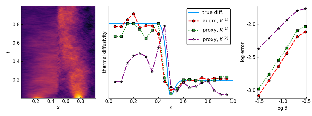 Figure 1