Classic and exotic Besov spaces induced by good grids
Daniel Smania

TL;DR
This paper explores Besov spaces defined via good grids, showing classical spaces are special cases and introducing exotic variants that differ from classical definitions.
Contribution
It demonstrates that classical Besov spaces on compact homogeneous spaces are examples of Besov spaces induced by good grids, and introduces exotic Besov spaces from interval partitions.
Findings
Classical Besov spaces are special cases of good grid-induced Besov spaces.
Exotic Besov spaces can differ from classical ones when defined by interval partitions.
The framework unifies and extends the understanding of Besov spaces on various measure spaces.
Abstract
In a previous work we introduced Besov spaces defined on a measure spaces with a good grid, with , and . Here we show that classical Besov spaces on compact homogeneous spaces are examples of such Besov spaces. On the other hand we show that even Besov spaces defined by a good grid made of partitions by intervals may differ from a classical Besov space, giving birth to exotic Besov spaces.
Click any figure to enlarge with its caption.
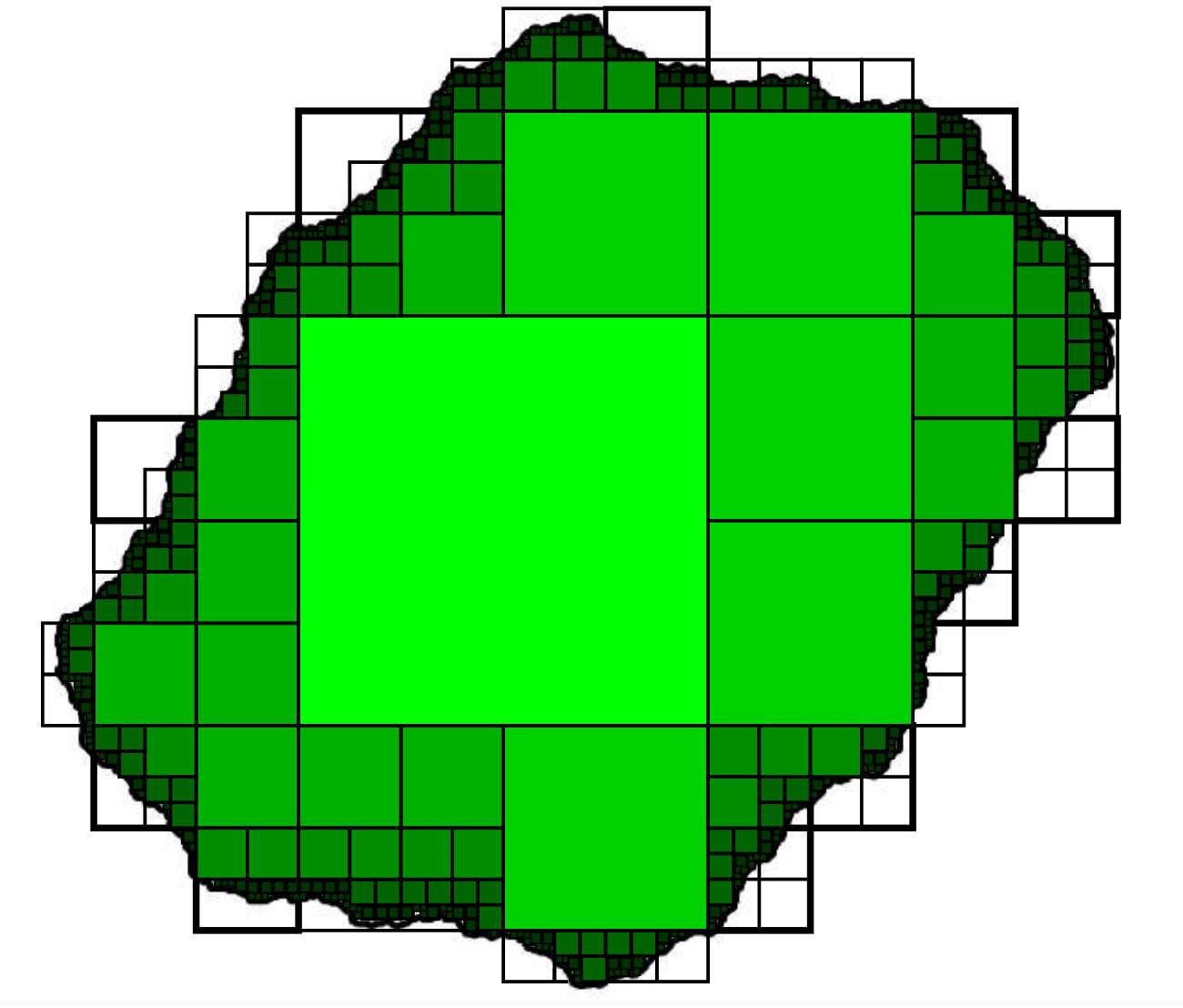 Figure 1
Peer Reviews
No public reviews on file for this paper yet. If you reviewed it on a platform where reviews are public (OpenReview, ICLR, NeurIPS, ICML), you can paste yours below so the community can read it here.
Videos
No videos yet. Explain this paper in a talk, walkthrough, or lecture? Add one.
\externaldocument
[besov-]besovish-2020-01-01
\newconstantfamilyc symbol=λ, format=0
\renewconstantfamilynormal symbol=C, format=0
\newconstantfamilye symbol=θ, format=0
\newconstantfamilyA symbol=A, format=0
\newconstantfamilyG symbol=G, format=0
Classic and exotic Besov spaces induced by good grids
Daniel Smania
Departamento de Matemática
Intituto de Ciências Matemáticas e da Computação-Universidade de São Paulo (ICMC/USP) - São Carlos
Caixa Postal 668
São Carlos-SP
CEP 13560-970
Brazil.
[email protected] http://conteudo.icmc.usp.br/pessoas/smania/
Abstract.
In a previous work we introduced Besov spaces defined on a measure spaces with a good grid, with , and . Here we show that classical Besov spaces on compact homogeneous spaces are examples of such Besov spaces. On the other hand we show that even Besov spaces defined by a good grid made of partitions by intervals may differ from a classical Besov space, giving birth to exotic Besov spaces.
Key words and phrases:
atomic decomposition, Besov space, harmonic analysis, wavelets
2010 Mathematics Subject Classification:
37C30, 30H25, 42B35, 42C15, 42C40
D.S. was partially supported by CNPq 307617/2016-5, CNPq 430351/2018-6, CNPq 306622/2019-0 and FAPESP Projeto Temático 2017/06463-3.
Contents
1. Introduction
We defined Besov spaces , with , and , on a measure spaces with a good grid [27]. Those spaces are defined by atomic decomposition using very simple atoms consisting of piecewise constant functions.
Similar but more general than Gu-Taibleson [14] recalibrated martingale Besov spaces, it allows us to carry results for classic Besov spaces in to measure spaces with a good grid, and often the proofs there are indeed simpler and more elementary. This includes results on multipliers, atomic decomposition and left and right compositions.
1.1. Measure spaces with good grids
A measure space with a good grid is a set endowed with a -algebra and a measure on , . For every measurable set denote . A good grid on is a sequence of finite families of measurable sets with positive measure so that
- i.
Every family is a partition of up to sets of zero measure.
- ii.
The family
[TABLE]
generates the -algebra .
- iii.
There is such that
[TABLE]
for all such that and for some .
1.2. Besov space on measure spaces with good grid
For each consider the function defined by
[TABLE]
for every and otherwise. The function is the Souza’s canonical atom on . The Besov space is the space of all functions in the Lebesgue space that can be represented by an absolutely convergent series on
[TABLE]
where and additionally
[TABLE]
The r.h.s. of (1.1) is a -representation of . Define
[TABLE]
where the infimum runs over all possible representations of as in (1.1). Then is a complex Banach space and its unit ball is compact in (see [27]).
1.3. Comparing Besov spaces
There is a large body of literature on Besov spaces. See Stein [28], Peetre [24], Triebel [31] and the references therein. Since Besov [4] defined Besov spaces in late 50’s, there is a long and ongoing quest to extend Besov spaces (and indeed harmonic analysis) to settings with weaker structure. Han and Sawyer [16] and Han, Lu and Yang [15] defined Besov spaces on homogeneous spaces. Those are a large class of quasi-metric spaces endowed with a doubling measure, introduced by Coifman and Weiss [8]. There are also definitions of Besov spaces on metric spaces and -sets. See Alvarado and Mitrea [2] and Koskela, Yang, and Zhou [19] and Triebel [32][30].
Our goal here is to compare the Besov spaces of a homogeneous space with the ones defined on a measure spaces with a good grid. While the former is certainly a far-reaching generalisation of Besov spaces on , the latter may at first glance looks like an artificial dyadic version of the classical Besov spaces, a sort of simplistic model of more complex situations. As it turn out, this couldn’t be farther from the truth.
Indeed there are earlier works that give atomic decompositions to classical Besov spaces where the atoms are piecewise constant functions. We cite the atomic decomposition of the Besov space , with , by de Souza [9] (see De Souza [10] and de Souza, O’Neil and Sampson [11]), some results on B-spline atomic decomposition of the Besov space of the unit cube of by DeVore and Popov [12], as well results on finite element approximation in bounded polyhedral domains on by Oswald [21] [22].
In part I, we consider compact homogeneous spaces, and using the famous dyadic ”cubes” constructed by Christ [7] (see also Hytönen and Kairema [17] for recent results on dyadic cubes in homogeneous spaces), we show that its Besov spaces, as defined by Han, Lu and Yang [15], are a particular case of the Besov spaces induced by grids. Note that Yang [35] already proved that Besov spaces on -sets defined by Triebel [32] also coincide with Besov spaces on these sets considering them as homogeneous spaces. We also observe that Gu-Taibleson recalibrated martingale Besov spaces [14] are Besov spaces of certain compact homogeneous spaces (see Section 3).
*Besov spaces on compact homogeneous spaces, with and small satisfying , and in particular recalibrated martingale Besov spaces, can be retrieved as particular examples of Besov spaces in measure spaces with a good grid. *
On the other hand in Part II we show that, even if we consider with a grid formed by a nested sequence of partitions by intervals, but that it is not ”recalibrated” as in Gu and Taibleson [14], then it may happens that the induced Besov space does *not * coincide with the Besov space of . Those ”exotic” Besov spaces are indeed useful to study certain transfer operators associated to expanding maps [3].
Yet our construction of Besov spaces with low regularity is likely to be the simplest construction available.
I. THE BEST OF ALL POSSIBLE WORLDS.
2. Besov spaces on compact homogeneous spaces
2.1. Homogeneous spaces
Let be a set. A quasi-metric in is a real-valued function in satisfying
- HS1.
We have ,
- HS2.
If then ,
- HS3.
We have ,
- HS4.
There exists such that
[TABLE]
For every the function is also a quasi-metric on . A quasi-metric is equivalent to if
[TABLE]
for some . We say that two quasi-metrics and are power-law equivalent if there exists such that is equivalent to .
A homogeneous space , introduced by Coifman and Weiss ****[8]****, is a topological space endowed with a quasi-metric and a borelian measure that satisfies
- HS5.
The measure is a doubling measure, that is, there is such that
[TABLE]
for every and .
Note that if is power-law equivalent to then is also a homogeneous space. By Macias and Segovia ****[20]****, replacing by an equivalent quasi-metric we can also assume
- HS6.
The quasi-balls , with , are open sets.
We will assume that for every , is compact and .
2.2. Induced Ahlfors regular quasi-metric space.
For every homogeneous space as in the previous section we can associated an Ahlfors regular quasi-metric space, that is, a triple , where is a quasi-metric, and
[TABLE]
provided , for some . Indeed is defined up to power law equivalence, but that will be enough to ours purposes.
Indeed by Macias and Segovia ****[20]**** if we define
[TABLE]
then is a quasi-metric on (that it is not necessarily equivalent to ) such that is a homogeneous space satisfying
[TABLE]
provided , for some , so is a Ahlfors regular quasi-metric space. Note that if and are power-law equivalent then the corresponding quasi-metrics and are equivalent.
**One may ask if there is a metric and such that is an Ahlfors regular *metric *** space and is power-law equivalent to . Indeed given such that we have that is a metric, where
[TABLE]
By Aimar, Iaffei and Nitti ****[1]**** and Paluszyński and Stempak ****[23]**** if then is a metric on , is a quasi-metric equivalent to . In particular and are power-law equivalent for every . Moreover
[TABLE]
for some and . So is a Ahlfors regular metric space.
2.3. Good grids in an Ahlfors regular quasi-metric space.
Due Section 2.2 from now on we will consider a general setting of Ahlfors regular quasi-metric space satisfying (2.4) for and some .
Proposition 2.1** (Good grids in Ahlfors regular quasi-metric spaces).**
There is a good grid such that for every quasi-metric that is power-law equivalent to the following holds: There is and such that for every , with , there is satisfying
[TABLE]
[TABLE]
and
[TABLE]
Proof.
By Christ [7] there is a family of partitions , , satisfying
- C1.
For every we have .
- C2.
For every we have either or .
- C3.
For every there is an unique such that .
- C4.
For every we have .
- C5.
For every there is such that , with .
- C6.
For every we have
[TABLE]
Let be such that
[TABLE]
and
[TABLE]
Let be such that
[TABLE]
Note that
[TABLE]
Let and for every . Then for every , and we have
[TABLE]
It is easy to see that has similar properties for every power-law equivalent metric . ∎
For every grid as in Proposition 2.1 we can consider the Banach space , using -Souza’s atoms, where , and .
Proposition 2.2**.**
Let be a grid as in Proposition 2.1 taking . Assume that . There is , such that the following holds. Let be an open subset such that there is satisfying
[TABLE]
and
[TABLE]
for some , , and . Then
- A.
The set is a -regular domain, with
[TABLE]
that is, there are families , such that
- i.
If , and then
- ii.
We have
[TABLE]
- iii.
We have
[TABLE]
- B.
We have for every and
[TABLE]
Proof.
Note that
[TABLE]
Let be the family of all such that and there is not satisfying . For every define
[TABLE]
otherwise set . Note that
[TABLE]
Here is the canonical -Souza’s atom on . If then
[TABLE]
Note also that if and
[TABLE]
then there is such that . Consequently if
[TABLE]
for some . It follows from (2.11) and (2.14) that
[TABLE]
Consequently by (2.11)
[TABLE]
This proves . Together with (2.13) we have that implies . ∎
Proposition 2.3**.**
Let , , be two grids as in Proposition 2.1 taking . Suppose that
[TABLE]
Then and the corresponding norms are equivalent.
Proof.
For each , denote by and the corresponding constants in Proposition 2.1. Fix . Given , let , where is the canonical Souza’s atom supported on . Let .
Claim I. We have
[TABLE]
where
[TABLE]
Indeed we have
[TABLE]
and if then
[TABLE]
In particular if and then , so and . In particular . On the other hand by (2.8)
[TABLE]
where
[TABLE]
Let be such that
[TABLE]
Then by (2.9) there is satisfying and , so (2.16) holds.
Claim II. There is such that
[TABLE]
By this follows from (2.8) and (2.9) taking
Claim III. There are such that
[TABLE]
holds.
Indeed, by Proposition 2.1 we have
[TABLE]
By (2.9) we have , so
[TABLE]
Claim II and III imply that we can apply Proposition 2.2 for and consequently is a -regular domain with respect the good grid , that is, one can find families as in Proposition 2.2 taking . For every define
[TABLE]
otherwise set . Note that
[TABLE]
and by Claim I
[TABLE]
with .
By Proposition LABEL:besov-trans.C in [27] we have that and there exists such that
[TABLE]
for every Exchanging the roles of and in the above argument we obtain the reverse inclusion and inequality. ∎
Definition 2.4**.**
Let be a homogeneous space and be a Ahlfors regular quasi-metric space such that is power-law equivalent to . Let be the supremum of all that admits a good grid as in Proposition 2.1 with . Let , and . Assume . We define the Besov space on the homogeneous space as . The Besov space is well-defined due Proposition 2.3.
Han, Lu and Yang ****[15]**** defined inhomogeneous Besov spaces for homogeneous spaces introducing a type of Calderón reproducing formula. They also obtained an atomic decomposition of these Besov spaces, that we describe now. Let as in (2.5) and be such that
[TABLE]
Note that is an Ahlfors regular quasi-metric space. Let be a grid as in Proposition 2.1 taking . Fix small enough such that as defined in (2.7) is a metric satisfying
[TABLE]
Let be such that . A Han-Lu-Yang -block associated to is a function
[TABLE]
such that
- i.
****
- ii.
****
- iii.
****
A function belongs to if (Theorem 2.1 and Proposition 3.1 in ****[15]****, and also Theorem 6.5 and Remark 6.20 in Han and Sawyer ****[16]****) we can write
[TABLE]
where is a Han-Lu-Yang -block associated to and the convergence is absolute in , that is
[TABLE]
and
[TABLE]
We define
[TABLE]
where the infimum runs over all possible representations (2.23). We are using a slightly different definition for an -block but we also modified the norm definition accordingly to obtain the same Besov space as in Han, Lu and Yang ****[15]****.
Proposition 2.5**.**
Let be a good grid as in Proposition 2.1 with . Suppose that , , and . Then .
Proof.
We will prove it in several steps.
Step I. Consider the grid
[TABLE]
Let be the class of atoms that consists of functions that satisfy
- i.
- ii.
- iii.
Note that there is such that for every
[TABLE]
This implies that and its norms are equivalent. We will prove that .
Step II. Let be the canonical -Souza’s atom on . We claim that for every , . Indeed for every , let be the family of all such that
- A.
We have
[TABLE]
- B.
If , with we have
[TABLE]
There is such that for every , with , we have
[TABLE]
In particular by (2.10) there is such that
[TABLE]
for every , and consequently
[TABLE]
for some constant . Note that
[TABLE]
For every such that define
[TABLE]
otherwise let . There is such that for every , , we have
[TABLE]
for every and
[TABLE]
for every . We claim that
[TABLE]
for every . Indeed, if then
[TABLE]
and if then
[TABLE]
In particular
[TABLE]
is a -block. Let
[TABLE]
Note that if and , since by (2.24) there is such that
[TABLE]
and consequently
[TABLE]
Finally note that due (2.6) and (2.8) there is such that for every , , we have
[TABLE]
and for every such that there is satisfying
[TABLE]
for some . As a consequence satisfies
[TABLE]
for every , with , . Moreover (2.26) and (2.27) implies
[TABLE]
for every . This implies that
[TABLE]
for every , with , . Then
[TABLE]
is a -block on and
[TABLE]
where So (2.29) implies that . So if is the canonical -Souza’s atom on then
[TABLE]
where
[TABLE]
Due (2.28)
[TABLE]
In particular .
Step III. We apply Proposition LABEL:besov-trans.C in [27] with , , and , and for every . We have that assumption (LABEL:besov-ad) in [27] follows from (2.30). Consequently
[TABLE]
and this inclusion is continuous.
Step IV. To prove the reverse continuous inclusion, note that there is such that for every , we have that , , where
[TABLE]
and
[TABLE]
There is such that the following holds. If then for every we have
[TABLE]
where are as defined in Section LABEL:besov-hatoms in [27] taking , and . So if
[TABLE]
is a -representation then define
[TABLE]
We have that
[TABLE]
and
[TABLE]
is a -representation of . Indeed
[TABLE]
So and
[TABLE]
Since by Proposition LABEL:besov-hold in [27] we have that and their norms are equivalent. The proof is complete. ∎
2.4. The case .
We would like to connect this abstract setting with classical Besov spaces on considering the very well-known homogeneous space , where is the euclidean metric on and is the Lebesgue measure on . Then is a Ahlfors regular quasi-metric space. Note that we can choose . Let be the partition of by -dimensional cubes with -dimensional faces with length which are parallels to the coordinate axes. Then is a good grid satisfying the conclusion of Proposition 2.1 when and taking and . By Proposition 2.3 we have that is well-defined provided , and . Proposition 2.5 implies that for every , and .
Consider the classical inhomogeneous Besov space of , with , and . Let
[TABLE]
We believe that it is well know that , however since we did not find a reference we provide a proof.
Proposition 2.6**.**
We have , for every , and .
Proof.
Fix . It follows from Frazier and Jawerth [13] that T is the set of all functions that can be written as in (1.1), where satisfy (1.2) and are functions in such that ,
[TABLE]
and
[TABLE]
for every In particular
[TABLE]
for some constant . Due the atomic decomposition of by Han, Lu and Yang [15] we conclude that (recall that ).
To show that we need to adapt the proof of Proposition 2.5, firstly considering all functions and balls defined in the whole (opposite to just on ). If we modify the definition of in Step I requiring additionally that all functions in there must be on then . Moreover on Step II. we need to modify the definition of to get a function on . Replace (2.25) by
[TABLE]
Since is just the euclidean distance and , with , is an euclidean ball, we have that is on and it satisfies all the estimates in the proof. Then we can carry out Step III to conclude that . ∎
3. Gu-Taibleson recalibrated martingale Besov spaces
Let be a compact Hausdorff space and let be a borelian measure such that . If is a good grid on , we can consider the recalibrated martingale Besov spaces as defined by Gu and Taibleson ****[14]****. In what follows, we just made the obvious adaptations of their definition to the compact setting. Instead of dealing directly with the good grid to define , Gu and Taibleson define a recalibration of the martingale structure as follows. A recalibration of is a new good grid such that
[TABLE]
and satisfying the following properties. If
[TABLE]
then
[TABLE]
and there exist such that
[TABLE]
and
[TABLE]
for every . By Gu and Taibleson ****[14]**** a recalibration always exists.
Given , define
[TABLE]
for every and
[TABLE]
Of course
[TABLE]
for every . Note that is exactly the function defined in (LABEL:besov-k0) in ****[27]****, if we replace by there. We say that that belongs to the Gu-Taibleson recalibrated martingale Besov space if
[TABLE]
Gu and Taibleson also proved that
[TABLE]
Proposition 3.1**.**
We have and its norms are equivalent.
Proof.
By Theorem LABEL:besov-alte in [27] we have
[TABLE]
On the other hand by (LABEL:besov-estphi) and Theorem LABEL:besov-alte in [27]
[TABLE]
∎
Following Gu and Taibleson, we can endow with the metric
[TABLE]
Then it is easy to see that is a 1-Ahlfors regular space, so in particular a homogeneous space. Indeed in this case , where and are as in (2.5) and (2.7). The following result is, as far as we know, new, and says that a Gu-Taibleson recalibrated martingale Besov spaces are particular examples of Besov spaces on homogenous spaces.
Theorem 3.2**.**
For small and the Gu-Taibleson recalibrated martingale Besov space does not depend on the chosen recalibration and it coincides with the Besov space of the homogeneous space .
Proof.
If is large enough and is small enough, there exists an increasing sequence such that
[TABLE]
for every . Define the new grid (which may not be a good grid) as for every and if One can easily prove using Proposition LABEL:besov-trans in [27] that and theirs norms are equivalent. Define the good grid as We have . Note that is a good grid as in Proposition 2.1 taking . Indeed (2.8) and (2.9) are easy to verify. Note that if and we have
[TABLE]
and so (2.10) holds and consequently (see Definition 2.4) we have . ∎
**We are going to see in Remark 7.3 that it is possible to choose the initial good grid is such way that *is not *** . That means that the families of spaces defined by Souza’s atoms is richer than the families of Besov spaces on homogeneous spaces and recalibrated martingale Besov spaces.
4. Examples of strongly regular domains
Let’s assume that is an Ahlfors quasi-metric space, such that (2.4) holds for every and . The following result give sufficient geometric conditions on for to be a strongly regular domain, and in particular for to define a multiplier in appropriated Besov spaces (see Section 4). This is obviously a generalisation of results in Triebel**[29]**** to our setting.**
Proposition 4.1**.**
Let be good grid for as in Proposition 2.1. Let be a closed subset such that is Ahlfors regular quasi-metric-space, with and some finite borelian measure , that is, for every and
[TABLE]
Then is a -strongly regular domain for some and satisfying
[TABLE]
that is, for every such that one can find families , , such that
- A.
We have
[TABLE]
- B.
If and then .
- C.
We have
[TABLE]
Suppose additionally that every element of is a connected set. Then every subset such that is also a -strongly regular domain.
Proof.
Suppose otherwise there is nothing to do. Define
[TABLE]
and for
[TABLE]
Given , let be such that . Note that Choose Then
[TABLE]
We claim that for every
[TABLE]
Here
[TABLE]
Indeed, suppose there is and such that , for every . In particular
[TABLE]
so
[TABLE]
and consequently This proves the claim. Choose . Then (4.34) and (4.35) implies
[TABLE]
Take
[TABLE]
Suppose now that every element of is a connected set and let be such that . Given let be the subfamily of all such that . Since is a connected set, if is not contained in we would have , which contradicts . So and in particular
[TABLE]
This easily implies that is also a -strongly regular domain. ∎
Remark 4.2**.**
The theory of conformal expanding dynamical systems provides plenty of examples of strongly regular domains on . For instance consider the Julia set of a hyperbolic polynomial. This is a compact subset, so let be a square such that . We endowed with a good grid generated by dyadic squares and the Lebesgue measure . The associated Besov space coincides with the Besov space of the homogenous space . Then supports a *geometric measure * that satisfies the assumptions of Proposition 4.1. See Przytycki and Urbański [25] and also the survey Urbański [33]. In particular every connected component of is a strongly regular domain of the homogenous space . We can consider for instance the Julia set of a quadratic polynomial , with small (see Figure 3.)
II. GETTING EAL.
5. Isometry with Besov spaces defined by intervals
A case that provides a very rich class of examples is when , is the Lebesgue measure and the good grid consists in sequences of partitions by intervals. It turns out that in the point of view of Banach spaces up to isometries, those Besov spaces are the only ones.
Proposition 5.1**.**
Let , with and , be a Besov-ish space defined on a probability space with a good grid . Then there is a good grid formed by partitions by intervals of such that, considering the Lebesgue measure on we have that the Banach space is isometric to .
Proof.
We can easy define a function that associated to each an interval such that
- i.
- ii.
If , with then .
- iii.
If with then .
Define and
[TABLE]
for every and . Then is well defined and it extends to an isometry
[TABLE]
It is easy to see that for every canonical Souza’s atom we have . Together with Proposition LABEL:besov-lp in [27] this implies that
[TABLE]
is well defined and an isometry. ∎
Corollary 5.2**.**
Let be a homogeneous space such that is compact and . Then the Besov space , with , and small, is isomorphic to the corresponding Besov space of the homogeneous space given by , the usual metric and the Lebesgue measure.
Proof.
It follows from Proposition 2.3 and Proposition 2.5. ∎
6. Quasisymmetric grids
In this section , is the Lebesgue measure and all grids consists in sequences of partitions by intervals. We say that a good grid consisting on sequence of partitions of by intervals is a -quasisymmetric grid if for every and satisfying we have
[TABLE]
Let be a closed interval in . Define
[TABLE]
Lemma 6.1**.**
The following holds.
- A.
Let be a -good grid. Then for every interval there are families of intervals such that
[TABLE]
is an interval. Moreover
[TABLE]
and
[TABLE]
for , and
[TABLE]
- B.
Suppose additionally that is a -quasisymmetric grid. There is such that for every interval and every and such that we have
[TABLE]
and for every we have
[TABLE]
Proof.
Let
[TABLE]
and
[TABLE]
Then
[TABLE]
If then and we define . Otherwise let be such that . If then and we define . Otherwise let be such that and . Of course and . Let
[TABLE]
with obvious adaptation if either or . Furthermore if is a -quasisymmetric grid then for every and such that we have
[TABLE]
and the same estimates holds replacing by . ∎
Proposition 6.2**.**
The following holds.
- A.
Let be a quasisymmetric map and be the grid of N-adic intervals. Then the grid defined by
[TABLE]
is a quasisymmetric grid.
- B.
On the other hand if is a quasisymmetric grid such that every has exactly children then there is a quasisymmetric function such that .
Proof of A.
If is a quasisymmetric map then there is such that (6.36) holds for every two intervals , with . In particular is a quasisymmetric grid. ∎
Proof of B.
Define as
[TABLE]
the function is well-defined since the sequence in the r.h.s. is non-decreasing and bounded by . It is easy to see that is monotone increasing and continuous, so it is a homeomorphism. Let , with . It follows from Lemma 6.1.A. that
[TABLE]
and
[TABLE]
Let , be such that . Due Lemma 6.1.B we have
[TABLE]
so
[TABLE]
On the other hand since is a quasisymmetric (and in particular good) grid we have
[TABLE]
so , where does not depend on and . By (6.37) and (6.38)
[TABLE]
so is a quasisymmetric map and consequently the same holds for . ∎
Proposition 6.3**.**
Let be a quasisymmetric -good grid and be an interval. There are families of intervals , , and increasing sequences such that
- A.
We have that
[TABLE]
is a countable partition of .
- B.
We have
[TABLE]
with
[TABLE]
- C.
There exists and such that
[TABLE]
for every , , , and for every , , .
- D.
We have
[TABLE]
Proof.
Let and
[TABLE]
We define families with , in the following way. Let
[TABLE]
and
[TABLE]
Let . By induction on define as the smallest such that
[TABLE]
and as the smallest such that
[TABLE]
and
[TABLE]
Note that
[TABLE]
for every and
[TABLE]
is a countable partition of .
Let be such that . Let be such that and . Since we have that
[TABLE]
Moreover since is a quasymmetric grid we have and for every . In particular
[TABLE]
and for every such that we have
[TABLE]
for every . We can use the same argument replacing by and by in the above argument. So C. holds. ∎
7. Exotic for
The goal of this section is to show how sensitive is the dependence of , for , with respect to the grid . Choosing distinct grids in a familiar space as , where is the Lebesgue measure, may give origin to distinct Besov-ish spaces. The reader should compare this result with Bourdaud and Sickel ****[6]**** and Bourdaud ****[5]****
Proposition 7.1**.**
Let , is the Lebesgue measure, and and be quasisymmetric grids such that for every , and we have
[TABLE]
Let be a quasisymmetric map such that . The following statements are equivalent.
- A.
We have .
- B.
We have .
- C.
The map is a bi-Lipchitz function.
Proof.
Without loss of generality we assume that and are -good grids. For an interval define
[TABLE]
[TABLE]
[TABLE]
We claim that
Claim 1. There is such that for every and satisfying we have .
and
Claim 2. There is such that for every , with , and satisfying we have
[TABLE]
Both Claims 1 and 2 follows easily from Lemma 6.1.
Claim 3. Suppose that
[TABLE]
Then is a bi-Lipchitz function.
Indeed if
[TABLE]
then Claim 2. implies that
[TABLE]
For every choose such that . Of course
[TABLE]
and
[TABLE]
so
[TABLE]
By Lemma 6.1.A each intersects at most intervals in , so intersects at most intervals in . Since covers we have
[TABLE]
so
[TABLE]
so there are constants such that
[TABLE]
Note that for every interval with we have
[TABLE]
so and consequently We conclude that
[TABLE]
so is bi-Lipchitz. This proves Claim 3.
Claim 4. If is a bi-Lipchitz function then .
Let . Then
[TABLE]
and consequently
[TABLE]
so
[TABLE]
for some that does not depend on . Let Consider Proposition 6.3 taking and let
[TABLE]
Then by Lemma 6.1.B we have
[TABLE]
with
[TABLE]
By Proposition LABEL:besov-trans.C in [27] we have . The proof of the reverse inclusion is similar.
Claim 5. Suppose that and
[TABLE]
Then there is .
Step I. Indeed this implies that for every we can find and families with elements , with and
[TABLE]
for every . Taking a subsequence we can also assume that is increasing, ,
[TABLE]
for every , and
[TABLE]
For every and choose such that . Note that Claim 1 implies
Step II. For every and let be the only children of . Define and let be the corresponding element of the unconditional basis in (note that in Claim 5 we have ) defined in Section LABEL:besov-haar in [27] using the grid . Then
[TABLE]
is the Haar representation of a function in . Indeed we have for , so
[TABLE]
So
[TABLE]
We conclude that , with .
Step III. Since, the ordering of the sum in (7.44) does not matter, so
[TABLE]
Since provided we have
[TABLE]
so .
Step IV. On the other hand, note that
[TABLE]
where
[TABLE]
and
[TABLE]
with
[TABLE]
[TABLE]
Here depends only on the geometry of , and . We have
[TABLE]
For every define
[TABLE]
where the families are as defined in Proposition 6.3 taking . Of course for , and for every we have , and consequently
[TABLE]
Moreover by Proposition 6.3.D
[TABLE]
Then
[TABLE]
Here is the canonical Souza’s atom on and
[TABLE]
Consequently
[TABLE]
So by Proposition LABEL:besov-trans.A in [27](take , and ) we have that . This completes the proof of Claim 5.
Claim 6. Suppose that and
[TABLE]
Then there is .
The proof of Claim 6. has many similarities with the proof of Claim 5., however there are modifications that may not seems obvious to the reader. We describe them below.
Step I. Consider families as in the Step I. in the proof of Claim 5, except that we replace condition (7.43) by
[TABLE]
and we also demand . For every and choose such that , and also satisfying . We have
Let be the only children of . Define and let be the corresponding element of the unconditional basis of , for every , defined in Section LABEL:besov-haar in [27] using the grid .
Step II. Define
[TABLE]
We claim that is well defined and it belongs to . Indeed, we can write
[TABLE]
where
[TABLE]
and
[TABLE]
with
[TABLE]
[TABLE]
So
[TABLE]
For every define
[TABLE]
where the families are as defined in Proposition 6.3 taking . Of course for , and for every we have , and consequently due Proposition 6.1.B
[TABLE]
Moreover
[TABLE]
Then
[TABLE]
Here is the canonical Souza’s atom on and
[TABLE]
Consequently
[TABLE]
So by Proposition LABEL:besov-trans.A in [27] (take , and ) we have that . In particular , for some .
Step III. In particular , for some . Since belongs to a unconditional basis of we can write
[TABLE]
Since , and for we conclude that
[TABLE]
so there is at least one such that
[TABLE]
We conclude that
[TABLE]
so .
This completes the proof of Claim 6.
To complete the proof of Proposition 7.1, note that Claim 4. tell us that and . Suppose that holds, that is . If then Claim 5. implies that (7.42) holds. So by Claim 3. we have that is a bi-Lipchitz function and Claim 4. gives . On the other hand if then Claim 6 (exchanging the roles of and ) implies that
[TABLE]
so again by Claim 3. we have that is a bi-Lipchitz function and Claim 4. gives . We conclude that and . Obviously , so this concludes the proof. ∎
Proposition 7.2** (Exotic Besov-ish spaces).**
Let be the Besov space of as defined in Section 2. There are quasisymmetric grids such that .
Proof.
Let and consider the smooth expanding map given by Note that the dyadic grid on is a sequence of Markov partitions for , that is, is a difeomorphism for every , with , and . Let be a to -covering of the circle such that . Then there is a quasisymmetric homeomorphism such that and conjugates and , that is, and on . In particular there is a quasisymmetric grid such that . We can choose in such way that for some there is some -periodic point of () satisfying
[TABLE]
We claim that is n͡ot a bi-Lipchitz map. Indeed, otherwise the conjugacy would be absolutely continuous with respect to the Lebesgue measure. But Shub and Sullivan [26] proved that every absolutely continuous conjugacy between two expanding maps on the circle is indeed a difeomorphism. But this is not possible since in this case it is easy to show that for every periodic point of . Since is not a bi-Lipchitz map, Proposition 7.1 (take and ) implies that . ∎
Remark 7.3**.**
One can ask if above is the Besov space of a homogenous space of the form , where is the Lebesgue measure and is some metric on other than the euclidean one. We do not have a complete answer for that. However note that can not be the metric defined in (3.32). Indeed, if we consider a recalibration of then we have that is a good grid of intervals where every interval in the same level as more of less the same length. Using the same argument of the proof of Theorem 3.2 we conclude that is the Besov space , where is the euclidean distance.
8. Good grid invariance for
The next result tell us that when the Besov spaces are far more resilient to modifications of the grid, what somehow remind us of Theorem 2.2 in Vodopyanov ****[34]****. See also Koch, Koskela, Saksman and Soto ****[18]****.
Proposition 8.1**.**
Consider the interval with the Lebesgue measure . Let be grids of such that
- A.
*We have that *are families of intervals for every ,
- B.
For every we have and
- C.
We have that is a -good grid.
Then
[TABLE]
and the inclusion is continuous. As a consequence , where is the Besov space in the homogeneous space .
Proof.
We will prove it in three steps.
Step I. Note that given two grids and such that
[TABLE]
for every , , and
[TABLE]
then and the corresponding norms are equivalent.
Define , with , in the following way.
[TABLE]
Then is a grid and consequently and the corresponding norms are equivalent. It remains to show the (continuous) inclusion .
Step II. Since is a good grid there is such that for every and there is , with , satisfying .
Step III. Given , define
[TABLE]
By Step II we have that . Let
[TABLE]
and
[TABLE]
and by induction define
[TABLE]
and
[TABLE]
Since is a nested sequence of partitions we can find a subfamily such that
[TABLE]
and is a family of pairwise disjoint intervals. By definition is a family of sets with pairwise disjoint interior. Note that
[TABLE]
can be described as
[TABLE]
Let be the convex hull of . If then
[TABLE]
so by Step II there is , with , such that Note that for every , otherwise we would have . In particular . Consequently
[TABLE]
Additionally if satisfies
[TABLE]
then by Step III there is , with , such that and which contradicts the inclusion . We conclude that
[TABLE]
so
[TABLE]
and for every satisfying we have
[TABLE]
so for every . If is the canonical Souza’s atom on and we have
[TABLE]
and for every
[TABLE]
By Propositon LABEL:besov-trans.C in [27] we have that and moreover this inclusion is continuous. In particular , and by Propostition 2.5 we have . ∎
The reference list from the paper itself. Each links out to its DOI / PubMed record.
- 1[1] H. Aimar, B. Iaffei, and L. Nitti. On the Macías-Segovia metrization of quasi-metric spaces. Rev. Un. Mat. Argentina , 41(2):67–75, 1998.
- 2[2] R. Alvarado and M. Mitrea. Hardy spaces on Ahlfors-regular quasi metric spaces , volume 2142 of Lecture Notes in Mathematics . Springer, Cham, 2015. A sharp theory.
- 3[3] A. Arbieto and D. Smania. Transfer operators and atomic decomposition. ar Xiv 1903.06943, 2019.
- 4[4] O. V. Besov. On some families of functional spaces. Imbedding and extension theorems. Dokl. Akad. Nauk SSSR , 126:1163–1165, 1959.
- 5[5] G. Bourdaud. Changes of variable in Besov spaces. II. Forum Math. , 12(5):545–563, 2000.
- 6[6] G. Bourdaud and W. Sickel. Changes of variable in Besov spaces. Math. Nachr. , 198:19–39, 1999.
- 7[7] M. Christ. A T ( b ) 𝑇 𝑏 T(b) theorem with remarks on analytic capacity and the Cauchy integral. Colloq. Math. , 60/61(2):601–628, 1990.
- 8[8] R. R. Coifman and G. Weiss. Analyse harmonique non-commutative sur certains espaces homogènes . Lecture Notes in Mathematics, Vol. 242. Springer-Verlag, Berlin-New York, 1971. Étude de certaines intégrales singulières.