Besov-ish spaces through atomic decomposition
Daniel Smania

TL;DR
This paper introduces new function spaces akin to Besov spaces using atomic decomposition in measure spaces with grids, providing insights into multipliers and compositions for low-regularity cases.
Contribution
It develops a novel approach to constructing Besov-like spaces via atomic decomposition in measure spaces with minimal assumptions.
Findings
New Besov-like spaces constructed using atomic decomposition.
Results on multipliers for low-regularity spaces.
Analysis of left compositions in the new spaces.
Abstract
We use the method of atomic decomposition to build new families of function spaces, similar to Besov spaces, in measure spaces with grids, a very mild assumption. Besov spaces with low regularity are considered in measure spaces with good grids, and results on multipliers and left compositions are obtained.
Click any figure to enlarge with its caption.
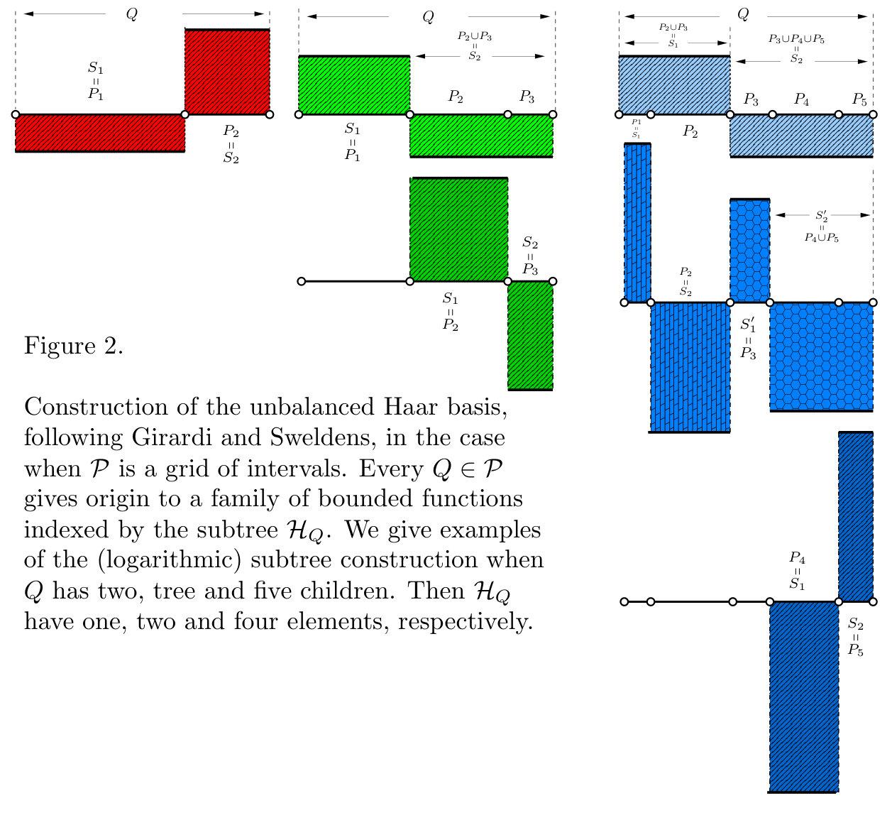 Figure 1
 Figure 2
 Figure 3
| Symbol | Description |
|---|---|
| phase space | |
| finite measure in the phase space | |
| an atom supported on P | |
| a class of atoms | |
| set of atoms of class supported on | |
| class of -Souza’s atoms | |
| class of -Hölder atoms | |
| class of -bounded variation atoms | |
| class of -Besov’s atoms | |
| grid of | |
| family subsets of at the -th level of | |
| describes geometry of the grid | |
| (s,p,q)-Banach space defined by the class of atoms | |
| or | (s,p,q)-Banach space defined by Souza’s atoms |
| elements of the grid | |
| or | Lesbesgue spaces of |
| norm in , | |
| , with . | |
| . | |
Peer Reviews
No public reviews on file for this paper yet. If you reviewed it on a platform where reviews are public (OpenReview, ICLR, NeurIPS, ICML), you can paste yours below so the community can read it here.
Videos
No videos yet. Explain this paper in a talk, walkthrough, or lecture? Add one.
\externaldocument
[homo-]besov-homo-2019-03-14
\newconstantfamilyc symbol=λ, format=0
\renewconstantfamilynormal symbol=C, format=0
\newconstantfamilye symbol=θ, format=0
\newconstantfamilyA symbol=A, format=0
\newconstantfamilyG symbol=G, format=0
Besov-ish spaces through atomic decomposition
Daniel Smania
Departamento de Matemática
Instituto de Ciências Matemáticas e de Computação-Universidade de São Paulo (ICMC/USP) - São Carlos
Caixa Postal 668
São Carlos-SP
CEP 13560-970
Brazil.
[email protected] https://sites.icmc.usp.br/smania/
Abstract.
We use the method of atomic decomposition to build new families of function spaces, similar to Besov spaces, in measure spaces with grids, a very mild assumption. Besov spaces with low regularity are considered in measure spaces with good grids, and we obtain results on multipliers and left compositions in this setting.
Key words and phrases:
atomic decomposition, Besov space, harmonic analysis, wavelets
2010 Mathematics Subject Classification:
37C30, 30H25, 42B35, 42C15, 42C40
We would like the thank the referee for the useful suggestions. D.S. was partially supported by CNPq 306622/2019-0, CNPq 307617/2016-5, CNPq Universal 430351/2018-6 and FAPESP Projeto Temático 2017/06463-3.
Contents
1. Introduction
inline,linecolor=blue,backgroundcolor=blue!25,bordercolor=blue,size=tiny,]Revision 1- We changed the abstract a little bit. Besov spaces were introduced by Besov [4]. This scale of spaces has been a favorite over linecolor=blue,backgroundcolor=blue!25,bordercolor=blue,size=tiny,]Revision 2- we replaced ”thought” by ”over” the years, with thousands of references available. Perhaps two of its most interesting features is that many earlier classes of function spaces appear linecolor=blue,backgroundcolor=blue!25,bordercolor=blue,size=tiny,]Revision 3- we replaced ”appears” by ”appear” in this scale, as Sobolev spaces, and also that there are many equivalent ways to define , in such way that you linecolor=blue,backgroundcolor=blue!25,bordercolor=blue,size=tiny,]Revision 4- we replaced ”in such way you” by ïn such way that you” can pick the more suitable one for your purpose. The reader may see Stein [43], Peetre [39], Triebel [47] for an introduction of Besov spaces on . For a historical account on Besov spaces and related topics, see Triebel [47] and the shorter linecolor=blue,backgroundcolor=blue!25,bordercolor=blue,size=tiny,]Revision 5- Replace ”more short” by ”shorter” but useful Jaffard [30], Yuan, Sickel and Yang [50] and Besov and Kalyabin [3].
In the last decades there was linecolor=blue,backgroundcolor=blue!25,bordercolor=blue,size=tiny,]Revision 6- we replaced ”were” by ”was” a huge amount of activity on the generalisation of harmonic analysis (see Deng and Han [17]), and Besov spaces in particular, to less regular phase spaces, replacing by something with a poorer structure. It turns out that for small and , a proper definition demands strikingly weak assumptions. There is a large body of literature that provides a definition and properties of Besov spaces on homogeneous spaces, as defined by Coifman and Weiss [12]. Those are quasi-metric spaces with a doubling measure, which includes in particular Ahlfors regular metric spaces. We refer to the linecolor=blue,backgroundcolor=blue!25,bordercolor=blue,size=tiny,]Revision 7- we replaced ”pionner”by ”pioneer”pioneer work of Han and Sawyer [28] and Han, Lu and Yang [27] for Besov spaces on homogeneous spaces and more recently Alvarado and Mitrea [1] and Koskela, Yang, and Zhou [33] (in this case for metric measure spaces) and Triebel [48][46] for Besov spaces on fractals. There is a long list of examples of homogeneous spaces in Coifman and Weiss [13]. The d-sets as defined in Triebel [48] are also examples of homogeneous spaces.
*We give a very elementary (and yet practical linecolor=blue,backgroundcolor=blue!25,bordercolor=blue,size=tiny,]Revision 8- we replaced ”pratical” by ”practical”) construction of Besov spaces , with and , for measure spaces endowed with a grid, that is, a sequence of finite partitions of measurable sets satisfying certain mild properties. *
This construction is close to the martingale Besov spaces as defined by Gu and Taibleson [25], however we deal with ”nonisotropic splitting” in our grid without applying the Gu-Taibleson recalibration procedure to our grid, which simplifies the definition and it allows a broader linecolor=blue,backgroundcolor=blue!25,bordercolor=blue,size=tiny,]Revision 9- we replaced ”wider” by ”broader” class of examples.
The linecolor=blue,backgroundcolor=blue!25,bordercolor=blue,size=tiny,]Revision 10- we replaced ”main” by ”primary” primary tool in this work is the concept of atomic decomposition. An atomic decomposition represents linecolor=blue,backgroundcolor=blue!25,bordercolor=blue,size=tiny,]Revision 11- we replaced ”is the representation of” by ”represents” each function in a space of functions as a (infinite) linear combination of fractions of the so-called atoms. The advantage of atomic decompositions is linecolor=blue,backgroundcolor=blue!25,bordercolor=blue,size=tiny,]Revision 12- we replaced ”in” by ”is” that the atoms are functions that are often far more regular than a typical element of the space. linecolor=blue,backgroundcolor=blue!25,bordercolor=blue,size=tiny,]Revision 13- we replaced ”But” by ”However” However a distinctive feature (compared with Fourier series with either Hilbert basis or unconditional basis) is that such atomic decomposition is in general not unique. Nevertheless, in a successful atomic decomposition of a normed space of functions, linecolor=blue,backgroundcolor=blue!25,bordercolor=blue,size=tiny,]Revision 14- comma added we can attribute a ”cost” to each possible representation, and the norm of the space is equivalent to the minimal cost (or infimum) among all representations. A function represented by a single atom has norm at most one, so the term ”atom” seems to be appropriated.
Coifman [11] introduced the atomic decomposition of the real Hardy space and Latter [35] found an atomic decomposition for The influential work of Frazier and Jawerth [22] gave us an atomic decomposition for the Besov spaces . In the context of homogeneous spaces, we have results by Han, Lu and Yang [27] on the linecolor=blue,backgroundcolor=blue!25,bordercolor=blue,size=tiny,]Revision 15- we included ”the” atomic decomposition of Besov spaces by Hölder atoms.
Closer to the spirit of this work we have the atomic decomposition of Besov space , with , by de Souza [14] using special atoms, that we call Souza’s atoms (see also De Souza [15] and de Souza, O’Neil and Sampson [16]). A Souza’s atom on an interval is quite simple, consisting of a function whose support is and is constant on .
We also refer to the results on the B-spline atomic decomposition of the Besov space of the unit cube of in DeVore and Popov [18] (with Ciesielski [10] as a precursor), that in the case reduces to an atomic decomposition by Souza’s atoms, and the work of Oswald [37] [38] on finite element approximation in bounded polyhedral domains on .
On the study of Besov spaces on and smooth manifolds, Souza’s atoms may seem to have setbacks that restrict its usefulness. They are not smooth, so it is fair to doubt the effectiveness of atomic decomposition by Souza’s atoms to obtain a better understanding of a partial differential equation or to represent data faithfully/without artifacts, a constant concern in applications of smooth wavelets (see Jaffard, Meyer and Ryan [31]).
On the other hand, in the study of ergodic properties of piecewise smooth dynamical systems, linecolor=blue,backgroundcolor=blue!25,bordercolor=blue,size=tiny,]Revision 16- comma inserted linecolor=blue,backgroundcolor=blue!25,bordercolor=blue,size=tiny,]Revision 17- we deleted ”the” transfer operators play linecolor=blue,backgroundcolor=blue!25,bordercolor=blue,size=tiny,]Revision 18- we replaced ”plays” by ”play” a huge role. Those operators act linecolor=blue,backgroundcolor=blue!25,bordercolor=blue,size=tiny,]Revision 19- we replaced ”acts” by ”act” on Lebesgue spaces , but they are more useful if one can show linecolor=blue,backgroundcolor=blue!25,bordercolor=blue,size=tiny,]Revision 20- we replaced ”it has a” by ”they have a” they have a (good) action on more regular function spaces. Unfortunately, linecolor=blue,backgroundcolor=blue!25,bordercolor=blue,size=tiny,]Revision 21- we included a comma in many cases the transfer operator does not preserve neither smoothness nor even continuity of a function. Discontinuities are a fact of life in this setting, and they do not go away as in certain dissipative PDEs, since the positive -eigenvectors of this operator, of utmost linecolor=blue,backgroundcolor=blue!25,bordercolor=blue,size=tiny,]Revision 22- repeated word ”importance” erased importance in its study, often have discontinuities themselves. The works of Lasota and Yorke [34] and Hofbauer and Keller [29] are landmark results in this direction. See also Baladi [2] and Broise [8] for more details. Atomic decomposition with Souza’s atoms, being the simplest possible kind of atom with discontinuities, might come in handy in these cases. That was a major motivation for this work.
Besides this fact, in an abstract homogeneous space higher-order linecolor=blue,backgroundcolor=blue!25,bordercolor=blue,size=tiny,]Revision 23- we replaced ”higher order” by ”higher-order” smoothness does not seem to be a very useful concept linecolor=blue,backgroundcolor=blue!25,bordercolor=blue,size=tiny,]Revision 24- comma removed since we can define just for small values of , so atomic decompositions by Souza’s atoms sounds far more attractive.
Indeed, the simplicity of Souza’s atoms allows linecolor=blue,backgroundcolor=blue!25,bordercolor=blue,size=tiny,]Revision 25- we replaced ”allow” by ”allows” us to throw away the necessity of a metric/topological structure on the phase space. We define Besov spaces on every measure space with a non-atomic linecolor=blue,backgroundcolor=blue!25,bordercolor=blue,size=tiny,]Revision 26- we replaced ”non atomic” by ”non-atomic” finite measure, provided we endowed it with a good grid. A good grid is just a sequence of finite partitions of measurable sets satisfying certain mild properties. We give the definition of Besov space on measure space with a (good) grid in Part II.
In linecolor=blue,backgroundcolor=blue!25,bordercolor=blue,size=tiny,]Revision 27- we replaced ”On” by ”In” the literature we usually see a known space of functions be described using atomic decomposition. This typically comes after a careful study of such space, and it is often a challenging task. More rare is the path we follow here. We start by *defining * the Besov spaces through atomic decomposition by Souza’s atoms. This construction of the spaces and the study of its basic properties, as its completeness and linecolor=blue,backgroundcolor=blue!25,bordercolor=blue,size=tiny,]Revision 28- we removed the extra ”its” compact inclusion in Lebesgue spaces, uses fairly general and simple arguments, and it does not depend on the particular nature of the atoms used, except for very mild conditions on its regularity. In Part I we describe this construction in full generality.
We construct Besov-ish spaces. There are far more general than Besov spaces. In particular, linecolor=blue,backgroundcolor=blue!25,bordercolor=blue,size=tiny,]Revision 29- we added a comma the nature of the atoms may change with its location and scale in the phase space and the grid itself can be very irregular.
The main result in Part I is Proposition 8.1. Due to linecolor=blue,backgroundcolor=blue!25,bordercolor=blue,size=tiny,]Revision 30- we added ”to” the generality of the setting, its statement is linecolor=blue,backgroundcolor=blue!25,bordercolor=blue,size=tiny,]Revision 31- we replaced ”hopeless” by ” hopelessly” hopelessly technical in nature, however this very powerful result has a simple meaning. Suppose we have an atomic decomposition of a function. If we replace each of those atoms by a combination of atoms (possibly of a different class) in such way that we linecolor=blue,backgroundcolor=blue!25,bordercolor=blue,size=tiny,]Revision 32- we replaced ”in such way we” by ”in such way that we” do not change the location of the support and also the ”mass” of the representation is concentrated linecolor=blue,backgroundcolor=blue!25,bordercolor=blue,size=tiny,]Revision 33- we replaced ”concentrate” by ”concentrated” pretty much on the same original scale, then we obtain a new atomic decomposition, and the cost of this atomic decomposition can be estimated linecolor=blue,backgroundcolor=blue!25,bordercolor=blue,size=tiny,]Revision 34- we replaced ”estimate” by ”estimated” by the cost of the original atomic decomposition. We will use this result many times throughout linecolor=blue,backgroundcolor=blue!25,bordercolor=blue,size=tiny,]Revision 35- we replaced ”along” by ”throughout” this work. This is obviously connected with almost diagonal operators as in Frazier and Jawerth [22][23].
In Part II we also offer a detailed analysis of the Besov spaces defined there. Since we define linecolor=blue,backgroundcolor=blue!25,bordercolor=blue,size=tiny,]Revision 36- we replaced ”defined” by ”define” it using combinations of Souza’s atoms, it is not clear a priori how rich are those spaces. So
We give a bunch of alternative characterisations of these Besov spaces. We show that using more flexible classes of atoms (piecewise Hölder atoms, -bounded variation atoms and even Besov atoms with higher regularity), we obtain the same Besov space. This often allows us to easily verify if a given function belongs to . We also have a mean oscillation characterisation in the spirit of Dorronsoro [19] and Gu and Taibleson [25], and we also obtained another one using Haar wavelets.
Haar wavelets were introduced by Haar [26] in the real line. The elegant construction of unbalanced Haar wavelets in general measure spaces with a grid by Girardi and Sweldens [24] will play an essential role here. If in general homogeneous spaces the Calderón reproducing formula appears to be the bit of harmonic analysis that survives in it and it allows to carry out the theory, in finite measure spaces with a good grid (and in particular *compact * homogenous spaces) full-blown Haar systems are alive and well. Recently a Haar system was used by Kairema, Li, Pereyra and Ward [32] to study dyadic versions of the Hardy and BMO spaces in homogeneous spaces.
We also provided a few applications in part III. In particular, linecolor=blue,backgroundcolor=blue!25,bordercolor=blue,size=tiny,]Revision 37- we added a comma we study the boundedness of pointwise multipliers acting in the Besov space. Since it is effortless linecolor=blue,backgroundcolor=blue!25,bordercolor=blue,size=tiny,]Revision 38- we replaced ”very easy” by ”effortless” to multiply Souza’s atoms, the proofs of these results are concise linecolor=blue,backgroundcolor=blue!25,bordercolor=blue,size=tiny,]Revision 39- we replaced ”very short” by ”concise” and easy to understand, generalising some of the results for Besov spaces in by Triebel[44] and Sickel [41]. We also study the boundedness of left composition in Besov spaces of measure spaces with a grid, similar to some results for in Bourdaud and Kateb [6] (see also Bourdaud and Kateb [5][7]).
It may come as a surprise to the reader that Besov spaces on compact homogeneous spaces as defined by Han, Lu and Yang [27] (and in particular Gu-Taibleson recalibrated martingale Besov spaces [25]) are indeed particular cases of Besov spaces defined here, provided and is small. We show this in a forthcoming work [42].
2. Notation
We will use for positive constants and for positive constants smaller than one.
I. DIVIDE AND RULE.
**
In Part I. we are going to assume , and
**
3. Measure spaces and grids
Let be a measure space with a -algebra and be a measure on , . Given a measurable set denote . We denote the Lebesgue spaes of by . A grid is a sequence of finite families of measurable sets with positive measure , so that at least one of these families is non empty and
- .
Given , let
[TABLE]
Then
[TABLE]
Define . To simplify the notation we also assume that for every and satisfying . We often abuse notation using for both and .
Remark 3.1**.**
There are plenty of examples of spaces with grids. Perhaps the simplest one is obtained considering with the Lebesgue measure and the dyadic grid given by
[TABLE]
We can also consider the dyadic grid of , endowed with the Lebesgue measure, given by
[TABLE]
and also the corresponding -adic grids replacing by in the above definitions. The above grids are somehow special since they are nested sequence of partitions of the phase space and all elements on the same level have linecolor=blue,backgroundcolor=blue!25,bordercolor=blue,size=tiny,]Revision 40- we replaced ”has” by ”have” exactly the same measure.
Remark 3.2**.**
Indeed, any measure space with a finite non-atomic measure can be endowed with a grid made of a nested sequence of partitions and such that all elements on the same level have linecolor=blue,backgroundcolor=blue!25,bordercolor=blue,size=tiny,]Revision 41- we replaced ”has” by ”have” linecolor=blue,backgroundcolor=blue!25,bordercolor=blue,size=tiny,]Revision 42- we replaced ”exactly” by ”precisely” precisely the same measure linecolor=blue,backgroundcolor=blue!25,bordercolor=blue,size=tiny,]Revision 43- we removed a comma since any such measure space is measure-theoretically the same that a finite interval with the Lebesgue measure.
Remark 3.3**.**
If we consider a (quasi)-metric space with a finite measure , we would like to construct ”nice” grids on . It turns out that if is a homogeneous space one can construct a nested sequence of partitions of the phase space and all elements on the same level are open subsets and have ”essentially” the same measure. This is an easy consequence of a remarkable linecolor=blue,backgroundcolor=blue!25,bordercolor=blue,size=tiny,]Revision 44- we replaced ’famous”by ”remarkable” result by Christ [9]. See [42].
Remark 3.4**.**
One can constructs grids for smooth compact manifolds and bounded polyhedral domains in using successive subdivisions of an initial triangulation of the domain (see for instance Oswald [37][38] ).
4. A bag of tricks.
Following closely the notation of Triebel ****[48]****, consider the set of all indexed sequences
[TABLE]
with , satisfying
[TABLE]
with the usual modification when . Then is a complex -Banach space with , that is, is a complete metric in
The following is a pair of arguments we will use across linecolor=blue,backgroundcolor=blue!25,bordercolor=blue,size=tiny,]Revision 45- we replaced ”along” by ”across” this paper to estimate norms in and . Those are very elementary, and we do not claim any originality. We collect them here to simplify the exposition. The reader can skip this for the cases , when the results bellow reduce to the familiar Hölder’s and Young’s inequalities. Their proofs were mostly based on ****[22, Proof of Theorem 3.1]****. Recall that for we defined .
Proposition 4.1** (Hölder-like trick).**
Let and . Let nonnegative sequences such that for every
[TABLE]
Then if we have
[TABLE]
and if
[TABLE]
where
- A.
*If and then if , *
and if .
- B.
If and then .
- C.
*If and then if , *
and if .
- D.
If and then .
Proof.
We have
Case A. If and , by the Hölder inequality for the pair
[TABLE]
Case B. If and then the triangular inequality for implies
[TABLE]
Case C. If and then and by the Hölder inequality for the pair
[TABLE]
Case D. if and then using the triangular inequality for
[TABLE]
∎
Proposition 4.2** (Convolution trick).**
Let . Let be such that for every
[TABLE]
Then
[TABLE]
where satisfies
- A.
If and then .
- B.
If and then .
- C.
If and then .
- D.
If and then
Proof.
We have
Case A. If and , by the Young’s inequality for the pair
[TABLE]
Case B. If and then the triangular inequality for and the Young’s inequality for the pair imply
[TABLE]
Case C. If and then by the Young’s inequality for the pair
[TABLE]
Case D. If and then using the triangular inequality for and the Young’s inequality for the pair
[TABLE]
∎
5. Atoms
**Let be a grid. Let , and . A family of atoms associated with of type is an indexed family of pairs where **
- .
** is a complex Banach space contained in .**
- .
If then for every .
- .
** is a convex subset of such that if and only if for every satisfying .**
- .
We have
[TABLE]
for every .
**We will say that is an -atom of type supported on and that is the local Banach space on . Sometimes we also assume **
- .
For every we have that is a compact subset in the strong topology of .
or
- .
**We have and every the set is a sequentially compact subset in the *weak *** topology of .
**or even **
- .
For every we have that is finite dimensional and contains a neighborhood of [math] in .
We provide examples of classes of atoms in Section 11.
6. Besov-ish spaces
Let , , , , be a grid and let be a family of atoms of type . We will also assume that
We have
[TABLE]
and
[TABLE]
The Besov-ish space is the set of all complex valued functions that can be represented by an absolutely convergent series on
[TABLE]
where is in , and with finite cost
[TABLE]
Note that the inner sum in (6.1) is finite. By absolutely convergence in we mean that
[TABLE]
The series in (6.1) is called a -representation of the function . Define
[TABLE]
where the infimum runs over all possible representations of as in (6.1).
Quite often along this work, when it is obvious the choice of the measure space and/or the grid we will write either or even instead of . Whenever we write just it means that we choose the Souza’s atoms , with parameters and , a class of atoms we properly define in Section 11.1.
Proposition 6.1**.**
Assume - and -. Let be such that
[TABLE]
and suppose
[TABLE]
Then for every coefficients satisfying (6.2) and every -atoms on the series (6.1) converges absolutely on . Indeed
[TABLE]
and
[TABLE]
Proof.
Firstly note that if
[TABLE]
Consequently
[TABLE]
By Proposition 4.1 (Hölder-like trick) and we have
[TABLE]
∎
Remark 6.2**.**
Note that due to linecolor=blue,backgroundcolor=blue!25,bordercolor=blue,size=tiny,]Revision 46- we added ”to” if then . Sometimes it is convenient to use sharper estimates than (6.5) and (6.6) replacing by the sequence
[TABLE]
For instance, if for every with , then we can replace by in (6.4). Here denotes the indicator function of the set .
Proposition 6.3**.**
Assume - and -. Then is a complex linear space and is a -norm, with . Moreover the linear inclusion
[TABLE]
is continuous.
Proof.
Le . Then there are -representations
[TABLE]
Let and otherwise. Of course
[TABLE]
where111We don’t need to worry so much if , since in this case and we can choose to be an arbitrary atom (for instance ) in such way that (6.7) holds. For this reason we are not going to explicitly deal with similar situations ( that is going to appear quite often) along the paper.
[TABLE]
and
[TABLE]
Note that are atoms due to linecolor=blue,backgroundcolor=blue!25,bordercolor=blue,size=tiny,]Revision 47- we added ”to” . So by we have that is also an atom, since it is a convex combination of atoms. In particular
[TABLE]
converges absolutely in to . It remains to prove that this is a -representation of . Indeed
[TABLE]
Taking the infimum over all possible -representations of and we obtain
[TABLE]
The identity is obvious. By Proposition 6.1 we have that if then , so , so is a -norm, moreover (6.6) tell us that is continuous. ∎
Proposition 6.4**.**
Assume - and -. Suppose that are functions in with -representations
[TABLE]
where is a -atom supported on , satisfying
- i.
There is such that for every
[TABLE]
- ii.
For every we have that exists.
- iii.
For every there is such that
- (1)
either the sequence converges to in the strong topology of , or 2. (2)
we have and weakly converges to .
then either strongly or weakly converges in , respectively, to , where has the -representation
[TABLE]
that satisfies
[TABLE]
Proof.
By (6.8) it follows that (6.10) holds and that (6.9) is indeed a -representation of a function . It remains to prove that converges to in in the topology under consideration. Given , fix large enough such that
[TABLE]
We can write
[TABLE]
where
[TABLE]
is an atom in , and
[TABLE]
Note that the series in the r.h.s. converges absolutely in . Of course
[TABLE]
So by (6.6) in Proposition 6.1 (see also Remark 6.2) we have
[TABLE]
In the case , note that if is large enough then
[TABLE]
and consequently . So strongly converges to .
In the case , given , with we have that for large enough
[TABLE]
and of course
[TABLE]
so weakly converges to in . ∎
Corollary 6.5**.**
Assume - and -, and
- (1)
either or 2. (2)
we have and .
Then
- i.
Let be such that for every . Then there is a subsequence that converges either strongly or weakly in , respectively, to some with .
- ii.
In both cases is a complex -Banach space, with ,
- iii
If holds then the inclusion
[TABLE]
is a compact linear inclusion.
Proof of i..
There are -representations
[TABLE]
where is a -atom supported on and
[TABLE]
and . In particular, . Since the set is countable, by the Cantor diagonal argument, taking a subsequence we can assume that for some . Due to linecolor=blue,backgroundcolor=blue!25,bordercolor=blue,size=tiny,]Revision 48- we added ”to” () and the Cantor diagonal argument, we can suppose that strongly (weakly) converges in to some . We set
[TABLE]
By Proposition 6.4 we conclude that with , and that converges to in . ∎
Proof of ii..
Let be a Cauchy sequence on . By Proposition 6.1 we have that is also a Cauchy sequence in . Let be its limit in . By Corollary 6.5.i have that . Note that for large and
[TABLE]
and converges to in , so again by Corollary 6.5.i we have that
[TABLE]
so converges to in . ∎
Proof of iii..
It follows from i. ∎
The proof of the following result linecolor=blue,backgroundcolor=blue!25,bordercolor=blue,size=tiny,]Revision 49- we replaced ”resukt” by ”result” is quite similar.
Corollary 6.6**.**
Assume - and -, and
- (1)
either or 2. (2)
we have and .
Then for every there is a -representation
[TABLE]
such that
[TABLE]
We refer to Edmunds and Triebel ****[20]**** for more information on compact linear transformations between quasi-Banach spaces.
Corollary 6.7**.**
Assume - and -. If for every we have that is finite-dimensional and is a closed subset of then is a -Banach space, with .
Proof.
Since all norms are equivalent in we have that implies that is a closed and bounded subset of , so it is compact. By Corollary 6.5.ii it follows that is a -Banach space. ∎
7. Scales of spaces
Note that a family of atoms of type induces an one-parameter scale
[TABLE]
where is the family of atoms of type defined by
[TABLE]
Moreover a family of atoms of type induces a two-parameter scale
[TABLE]
where is the family of atoms of type defined by
[TABLE]
Proposition 7.1**.**
Assume -. Suppose that the -atoms satisfy -. Let and . Suppose
[TABLE]
Then
- A.
We have and the inclusion is a continuous linear map.
- B.
Suppose that also satisfies . Let be such that for every . Then there is a subsequence that converges in to some with .
- C.
Suppose that also satisfies . The inclusion is a compact linear map.
Proof.
Consider a -representation
[TABLE]
Since is an -atom, we have that is an -atom. In particular, we can write
[TABLE]
If then
[TABLE]
so
[TABLE]
Proof of A. In particular, linecolor=blue,backgroundcolor=blue!25,bordercolor=blue,size=tiny,]Revision 50- we added a comma taking we conclude that and
[TABLE]
Proof of B. By definition, there exist , such that
[TABLE]
where is a -atom supported on and
[TABLE]
where . In particular, . Since the set is countable, by the Cantor diagonal argument, taking a subsequence we can assume that and (due to linecolor=blue,backgroundcolor=blue!25,bordercolor=blue,size=tiny,]Revision 51- we added ”to” ) that converges in and to some . By Lemma 6.4 the sequence converge in to a function such that and with -representation
[TABLE]
It remains to show that the convergence indeed occurs in the topology of . For every and we can write
[TABLE]
where
[TABLE]
and with given by
[TABLE]
and
[TABLE]
Note that . Given , choose such that . Given , choose such that
[TABLE]
By (7.12) and (7.13) for each large enough we have
[TABLE]
In particular
[TABLE]
Choose such that
[TABLE]
Due to linecolor=blue,backgroundcolor=blue!25,bordercolor=blue,size=tiny,]Revision 52- we added ”to” there is such that for every , with , if satisfies then . Since in we conclude that for large enough we have
[TABLE]
for every , with . In particular
[TABLE]
We conclude that
[TABLE]
for large enough, so the sequence converges (due to linecolor=blue,backgroundcolor=blue!25,bordercolor=blue,size=tiny,]Revision 53- we added ”to” Corollary 6.5) to in the topology of .
∎
8. Transmutation of atoms
It turns out that sometimes a Besov-ish space can be obtained using different classes of atoms. The key result in Part I is the following
Proposition 8.1** (Transmutation of atoms).**
*Assume
- I.
Let be a class of -atoms for a grid , satisfying -* and -. Let be also a grid satisfying -.*
- II.
Let for be a sequence such that there is and satisfying
[TABLE]
for every .
- III.
There is such that the following holds. For every and satisfying there are atoms and corresponding such that
[TABLE]
is a -representation of a function , with for every , with and moreover
[TABLE]
*for every . *
Let
[TABLE]
*Then
- A.
For every coefficients such that
[TABLE]
we have that the sequence
[TABLE]
converges in to a function in that has a -representation
[TABLE]
where for every and
[TABLE]
Here and is defined by
[TABLE]
- B.
Suppose that the assumptions of A. hold and that are non negative real numbers and on for every . Then and on imply that for some satisfying and . If we additionally assume that for every then also implies on .
- C.
Let be a class of -atoms for the grid satisfying -. Suppose that there is such that for every atom we can find and in III. such that . Then
[TABLE]
and this inclusion is continuous. Indeed
[TABLE]
for every
inline,linecolor=blue,backgroundcolor=blue!25,bordercolor=blue,size=tiny,]Revision 54- In the caption of the figure 1 we replaced ”are concentrated” by ”concentrates”
Proof.
For every , with , and define
[TABLE]
Due to linecolor=blue,backgroundcolor=blue!25,bordercolor=blue,size=tiny,]Revision 55- we added ”to” this sum has a finite number of terms. If this sum has zero terms define and let be the zero function. Otherwise define
[TABLE]
We have that is an -atom.
Claim I. We claim that for
[TABLE]
Note that if then due to linecolor=blue,backgroundcolor=blue!25,bordercolor=blue,size=tiny,]Revision 56- we added ”to” (6.5), with and (8.14) we have
[TABLE]
Consequently we can do the following manipulation in
[TABLE]
This concludes the proof of Claim I.
Claim II. For every we claim that
[TABLE]
*is a -representation and *
[TABLE]
Indeed
[TABLE]
If and then this is a convolution, so we can use Proposition 4.2 (the convolution trick) and it easily follows (8.17). In the general case, consider
[TABLE]
Every can be written in an unique way as , with , , and . Fix and . Then there is at most one such that and . Indeed, if and , with and and smaller than , then , so and . If such exists, denote and and . Otherwise let . Then (8.21) implies
[TABLE]
Here if , and otherwise. Fixing , Proposition 4.2 (the convolution trick) gives us
[TABLE]
and
[TABLE]
This implies in particular that the sum in (8.19) is a -representation. This proves Claim II.
Claim III. We have that in the strong topology of
[TABLE]
For each the sequence
[TABLE]
is eventually constant, therefore convergent. The same happens with
[TABLE]
Estimate (8.20) and Proposition 6.4 imply that that (8.15) converges in to a function with -representation (8.19) with . This concludes the proof of Claim III.
Then Claim I, II, and III imply A. taking and We have that C. is an immediate consequence of A. Note that (8.18) and A. give B. ∎
9. Good grids
A -good grid , with , is a grid with the following properties:
We have .
We have (up to a set of zero -measure).
The elements of the family are pairwise disjoint.
For every and there exists such that .
We have
[TABLE]
for every satisfying and for some .
The family generate the -algebra .
10. Induced spaces
Consider a Besov-ish space , where is a good grid. Given , we can consider the sequence of finite families of subsets of given by
[TABLE]
Let be the restriction of the indexed family of pairs to indices belonging to . Then we can consider the induced Besov-ish space . Of course the inclusion
[TABLE]
is well-defined linecolor=blue,backgroundcolor=blue!25,bordercolor=blue,size=tiny,]Revision 57- we replaced ”well defined”by ”well-defined” and it is a weak contraction, that is
[TABLE]
Under the degree of generality we are considering here, the restriction transformation
[TABLE]
given by , is a bounded linear transformation, however it is easy to find examples of Besov-ish spaces where
11. Examples of classes of atoms.
There are many classes of atoms one may consider. We list here just a few of them.
11.1. Souza’s atoms
Let . A -Souza’s atom supported on is a function such that for every and is constant on , with
[TABLE]
The set of Souza’s atoms supported on will be denoted by A canonical Souza’s atom on is the Souza’s atom such that for every . Souza’s atoms are -type atoms.
11.2. Hölder atoms
Suppose that is a quasi-metric space with a quasi-distance , such that every is a bounded set and there is such that
[TABLE]
for every with and . Additionally assume that there is and such that
[TABLE]
Let
[TABLE]
For every , Let be the Banach space of all functions such that for , and
[TABLE]
Let be the convex subset of all functions satisfying
[TABLE]
We say that is the set of -Hölder atoms supported on . Of course -atoms are -type atoms and .
11.3. Bounded variation atoms
Now suppose that is an interval of with length , is the Lebesgue measure on it and the partitions in the grid are partitions by intervals. Let be an interval and , . A -bounded variation atom on is a function such that for every ,
[TABLE]
and
[TABLE]
Here is the pseudo-norm
[TABLE]
where the sup runs over all possible sequences , with in the interior of . We will denote the set of bounded variation atoms on as . Bounded variation atoms are also -type atoms.
II. SPACES DEFINED BY SOUZA’S ATOMS.
**
In Part II. we suppose that , and .
**
12. Besov spaces in a measure space with a good grid
We will study the Besov-ish spaces associated with the measure space with a good grid . We denote . Note that satisfies -. Note that by Proposition 6.1 there is such that .
If , and we wil say that is a Besov space.
13. Positive cone
We say that is -positive if there is a -representation
[TABLE]
where and is the standard -Souza’s atom supported on . The set of all -positive functions is a convex cone in , denoted . We can define a “norm” on as
[TABLE]
where the infimum runs over all possible -positive representations of . Of course for every and we have
[TABLE]
Moreover if is a real-valued function then one can find such that and
[TABLE]
An obvious but important observation is
Proposition 13.1**.**
if then its support
[TABLE]
is (up to a set of zero measure) is a countable union of elements of .
14. Unbalanced Haar wavelets
Let be a good grid. For every let , , be the family of elements such that for every , and ordered in some arbitrary way. The elements of will be called children of . Note that every has at least two children. We will use one of the method described (Type I tree with the logarithmic subtrees construction) in Girardi and Sweldens ****[24]**** to construct an unconditional basis of , for every .
Let be the family of pairs , with and , defined as
[TABLE]
where are constructed recursively in the following way. Let , where and . Here denotes the integer part of . Suppose that we have defined . For each element , fix an ordering and . For each such that , define and and add to . This defines
Note that since is a good grid we have for large and indeed
[TABLE]
Define . For every define
[TABLE]
where
[TABLE]
Note that
[TABLE]
Since we have
[TABLE]
so
[TABLE]
Consequently
[TABLE]
for every Here
[TABLE]
Let
[TABLE]
and define
[TABLE]
Then by Girardi and Sweldens ****[24]**** we have that
[TABLE]
is an unconditional basis of for every .
15. Alternative characterizations I: Messing with norms.
We are going to describe three norms that are equivalent to . Their advantage is that they are far more concrete, in the sense that we do not need to consider arbitrary atomic decompositions to define them.
15.1. Haar representation
For every , , the series
[TABLE]
is converges unconditionally in , where We will call the r.h.s. of (15.26) the Haar representation of . Define
[TABLE]
15.2. Standard atomic representation
Note that
[TABLE]
where and is the canonical Souza’s atom on . Let . Then , with and some , with . It is easy to see that for every the function
[TABLE]
is a Souza’s atom on . Choose
[TABLE]
Note that
[TABLE]
For every child of , , define
[TABLE]
where
[TABLE]
The (finite) number of terms on this sum depends only on the geometry of . Then is a Souza’s atom on and
[TABLE]
Let be the canonical -Souza’s atom on and choose . Denote
[TABLE]
In particular, linecolor=blue,backgroundcolor=blue!25,bordercolor=blue,size=tiny,]Revision 58- we added a comma for every
[TABLE]
extends to a bounded linear functional in . We have and
[TABLE]
where this series converges unconditionally in . Here is the canonical Souza’s atom. We will call the r.h.s. of (15.29) the standard atomic representation of . Let
[TABLE]
15.3. Mean oscillation
Define for
[TABLE]
and
[TABLE]
Denote for every and
[TABLE]
with the obvious adaptation for . Let
[TABLE]
15.4. These norms are equivalent
We have
Theorem 15.1**.**
Suppose , and . Each one of the norms , , , is finite if and only if . Furthermore these norms are equivalent on . Indeed
[TABLE]
[TABLE]
[TABLE]
[TABLE]
where
[TABLE]
[TABLE]
Proof.
The inequality (15.31) is obvious. To simplify the notation we write instead of .
Proof of (15.32). The number of terms in the r.h.s. of (15.28) depends only on the geometry of . Indeed
[TABLE]
Consider the standard atomic representation of given by (15.29). Note that by (15.27)
[TABLE]
for every . Consequently
[TABLE]
This completes the proof of (15.32).
Proof of (15.33). Note that
[TABLE]
Given and , choose such that
[TABLE]
Since has zero mean on for every we have
[TABLE]
Since is arbitrary, this concludes the proof of (15.33).
Proof of (15.34). Finally note that if and then there is a -representation of
[TABLE]
such that
[TABLE]
For each , choose . Then
[TABLE]
This is a convolution, so
[TABLE]
and since is arbitrary, by Proposition 6.1 we obtain
[TABLE]
This proves (15.34). ∎
The following is an important consequence of this section.
Corollary 15.2**.**
For each there exists a linear functional in
[TABLE]
with the following property. The so-called standard -representation of given by
[TABLE]
satisfies
[TABLE]
16. Alternative characterizations II: Messing with atoms.
Here we move to alternative descriptions of , linecolor=blue,backgroundcolor=blue!25,bordercolor=blue,size=tiny,]Revision 59- we added a comma which are quite different from linecolor=blue,backgroundcolor=blue!25,bordercolor=blue,size=tiny,]Revision 60- we replaced preposition ”of” by ”from” those in Section 15. Instead of choosing a definitive representation of elements of , linecolor=blue,backgroundcolor=blue!25,bordercolor=blue,size=tiny,]Revision 61- we added a comma we indeed give atomic decompositions of using far more general classes of atoms.
16.1. Using Besov’s atoms
The advantage of Besov’s atoms is that it is a wide and general class of atoms, that includes even unbounded functions. They can be considered in every measure space endowed with a good grid as in Section 3. Moreover in appropriate settings it contains Hölder and bounded variations atoms, which will be quite useful in the get other characterizations of . The atomic decompositions of by Besov’s atoms were considered by Triebel ****[45]**** in the case , and by Schneider and Vybíral ****[40]**** in the case , . They are refered there as ”non-smooth atomic decompositions”.
Let and . A -Besov atom on the interval is a function such that for , and
[TABLE]
where
[TABLE]
The family of -Besov atoms supported on will be denoted by . Naturally . By Proposition 6.1 we have
[TABLE]
**so a -Besov atom is an atom of type . **
The following result says there are many ways to define using various classes of atoms.
Proposition 16.1** (Souza’s atoms and Besov’s atoms).**
Let be a good grid. Let be a class of -atoms , with , such that for some , , and , we have that for every
[TABLE]
Then
[TABLE]
Moreover
[TABLE]
Proof.
The first inequality is obvious. To prove the second inequality, recall that due to linecolor=blue,backgroundcolor=blue!25,bordercolor=blue,size=tiny,]Revision 62- we added ”to” Proposition 8.1 it is enough to show the following claim
Claim. Let be a -Besov atom on . Then for every with there is such that
[TABLE]
where is the canonical -Souza’s atom on and
[TABLE]
Indeed, since
[TABLE]
there exists a -representation
[TABLE]
where is the canonical -Souza’s atom on and
[TABLE]
Then
[TABLE]
is a -Souza’s atom and
[TABLE]
with and
[TABLE]
∎
16.2. Using Hölder atoms
Suppose that is a quasi-metric space with a quasi-distance and a good grid satisfying the assumptions in Section 11.2.
Proposition 16.2**.**
Suppose
[TABLE]
* and For every we have*
[TABLE]
for some . Moreover
[TABLE]
for some In particular
[TABLE]
and the corresponding norms are equivalent.
Proof.
Let . Then has a continuous extension to . So firstly we assume that has a continuous extension to . Define
[TABLE]
and for every with and define
[TABLE]
Of course in this case and
[TABLE]
Here Consequently
[TABLE]
so
[TABLE]
This implies that
[TABLE]
where is the canonical -atom on , is a -representation of a function . From (16.41) it follows that
[TABLE]
for every In particular
[TABLE]
for almost every , so . So
[TABLE]
where
[TABLE]
In the general case, note that and . Applying (16.43) to and we obtain (16.38).
The second inclusion (16.39) in the proposition can be obtained taking in (16.2) and a few modifications in the above argument. By Proposition 16.1 we have (16.40). ∎
16.3. Using bounded variation atoms
Now suppose that is an interval of of length , is the Lebesgue measure on it and the partitions in are partitions by intervals.
Proposition 16.3**.**
If
[TABLE]
then
[TABLE]
for every If
[TABLE]
then
[TABLE]
for every . In particular
[TABLE]
and the corresponding norms are equivalents.
Proof.
Suppose
[TABLE]
Let and . We have
[TABLE]
where Note that for every
[TABLE]
Note that in the case the argument above needs a simple modification. For let be such that . Then
[TABLE]
By Theorem 15.1 we have that if then for some , and if we have that for every
[TABLE]
so for some . ∎
17. Dirac’s approximations
We will use the Haar basis and notation defined by Section 14. For every and define the finite family
[TABLE]
Let . Then we can enumerate the elements
[TABLE]
of such that satisfies
[TABLE]
for some and
[TABLE]
for every . Let
[TABLE]
and define for
[TABLE]
One can prove by induction on that for
[TABLE]
and in particular
[TABLE]
where In other words
[TABLE]
Note that
[TABLE]
Multiplying (17.44) by and integrating it term by term, and using (17.45) we obtain
[TABLE]
If , with , it can be written as
[TABLE]
with , where this series converges unconditionally on . Let
[TABLE]
Then
[TABLE]
Let
[TABLE]
be the series given by (15.29). Note that
[TABLE]
Consequently
Proposition 17.1** (Dirac’s Approximations).**
Let , with . Let
[TABLE]
- A.
If this representation is either as in (15.29) or for every then we have For every
[TABLE]
- B.
In the case of the representation (15.29) we also have
[TABLE]
Proof.
We have that is obvious if for every . In the other case note that for every we have
[TABLE]
so A. and B. follows. ∎
III. APPLICATIONS.
**
In Part III. we suppose that , and .
**
18. Pointwise multipliers acting on
Here we will apply the previous sections to study pointwise multipliers of . To be more precise, Let be a measurable function. We say that is a pointwise multiplier acting on if the transformation
[TABLE]
defines a bounded operator in . We denote the set of pointwise multipliers by . We can consider the norm on given by
[TABLE]
Of course a necessary condition for a function to be a multiplier is that
[TABLE]
Denote
[TABLE]
The linear space endowed with is a normed space introduced by Triebel ****[45]****. We have
[TABLE]
In the following three propositions we see that many results of Triebel ****[45]**** and Schneider and Vybíral ****[40]**** for Besov spaces in can be easily moved to our setting. The simplest case occurs when .
Proposition 18.1**.**
We have that .
Proof.
Let Given and one can find a -representation
[TABLE]
where is a -Souza’s atom and
[TABLE]
so
[TABLE]
and consequently
[TABLE]
Since is arbitrary we get
[TABLE]
∎
Lemma 18.2**.**
Let . The restriction application
[TABLE]
given by is continuous. Indeed there is , that does not depend on , such that
- A.
For every we have
[TABLE]
In particular . 2. B.
For every -representation
[TABLE]
one can find a -representation
[TABLE]
such that
[TABLE]
Moreover implies .
Proof.
Let Denote by the canonical -Souza’s atom supported on . If we can write If then If then
[TABLE]
where
[TABLE]
In every case we can write
[TABLE]
with
[TABLE]
By Proposition 8.1.A and 8.1.B there is such that A. and B. hold. ∎
Proposition 18.3**.**
We have that and this inclusion is continuous.
Proof.
Let . Then and by Lemma 18.2 we have
[TABLE]
By Proposition 6.1 (taking t = ) we have -Souza’s atom we have
[TABLE]
for some constant . In other words
[TABLE]
so
[TABLE]
for every . Due to the fact that generates the -algebra , by Lévy’s Upward Theorem (see Williams [49]) for almost every the following holds. If then
[TABLE]
So
[TABLE]
∎
inline,linecolor=blue,backgroundcolor=blue!25,bordercolor=blue,size=tiny,]Revision 63- In the caption of Figure 2, we replaced ”. the” by ”. The” (missing capitalization) and we replaced ”contributing for” by ”contribution to”
18.1. Non-Archimedean behaviour in
If we have a sequence we can get the naive estimate
[TABLE]
Nevertheless linecolor=blue,backgroundcolor=blue!25,bordercolor=blue,size=tiny,]Revision 64- we replaced ”But it is remarkable that” by ”Nevertheless, remarkably,”, remarkably, sometimes one can get a far better estimate. To state the result we need to define
[TABLE]
It is easy to see that this norm is equivalent to .
Proposition 18.4**.**
Let . There is with the following property. Let , with , and .
Consider a function with a -representation
[TABLE]
satisfying
- A.
We have
[TABLE]
- B.
If satisfies and then .
Then we can find a -representation
[TABLE]
such that
[TABLE]
Proof.
It is enough to prove the result for the case when is finite. Let with . There is , such that
[TABLE]
and for every . In particular By Lemma 18.2 for each we can find a -representation
[TABLE]
such that is the canonical -Souza’s atom supported on and
[TABLE]
Since , where is the canonical -Souza’s atoms supported on , we can write
[TABLE]
with satisfying
[TABLE]
so we can write
[TABLE]
with
[TABLE]
satisfying
[TABLE]
By Proposition 8.1.A we can find a -representation (18.51) satisfying (18.4). ∎
Remark 18.5**.**
If is -positive we can define
[TABLE]
If we assume additionally that are -positive, Proposition 18.4 remains true if we replace all the instances of by in its statement. Moreover by Proposition 8.1.B and Lemma 18.2. B we can conclude that
- i.
if for every then for every ,
- ii.
If is such that then , for some .
Corollary 18.6**.**
For every and we have . Moreover this inclusion is continuous.
18.2. Strongly regular domains
We may wonder on which conditions the characteristic function of a set is a pointwise multiplier in .
Definition 18.7**.**
A measurable set is a -strongly regular domain if for every , with , there is family such that
- i.
We have .
- ii.
If and then .
- iii.
We have
[TABLE]
The following result can be associated with results in Triebel ****[45]**** for , especially linecolor=blue,backgroundcolor=blue!25,bordercolor=blue,size=tiny,]Revision 65- we replaced ”specially” by ”especially” when we consider the setting of Besov spaces in compact homogenous spaces. See Section 18.2 for details.See also Schneider and Vybíral ****[40]****.
Proposition 18.8**.**
If is a -strongly regular domain then
[TABLE]
Proof.
Given , with we can write
[TABLE]
where is a -atom. Note that
[TABLE]
so (18.56) holds. ∎
Proposition 18.9** (Pointwise Multipliers I).**
There is with the following property. Suppose that are -strongly regular domains, , and for every . Consider a function with a -representation
[TABLE]
satisfying
- A.
We have
[TABLE]
- B.
If satisfies and then .
Then we can find a -representation
[TABLE]
such that
[TABLE]
Moreover
- i.
If satisfies then for some .
- ii.
If for every then for every .
Proof.
It follows from Proposition 18.4, Proposition 18.8 and Remark 18.5. ∎
18.3. Functions on
We want linecolor=blue,backgroundcolor=blue!25,bordercolor=blue,size=tiny,]Revision 66- ”we replaced ”We would like to give” by ”We want to give” to give explicit examples of multipliers in . One should compare the following result with the study by Triebel**[44]**** of the regularity of the multiplication on Besov spaces. See also Maz’ya and Shaposhnikova [36] for more information on multipliers in classical Besov spaces.**
Proposition 18.10** (Pointwise multipliers II).**
Let . Then the multiplier operator
[TABLE]
defined by is a well-defined linecolor=blue,backgroundcolor=blue!25,bordercolor=blue,size=tiny,]Revision 67- we replaced ”well defined” by ”well-defined” and bounded operator acting on . Indeed
[TABLE]
where and are as in Corollary 15.2.
Remark 18.11**.**
We can get a similar result replacing by everywhere.
Proof.
Let be the canonical -Souza’s atom on and be the canonical -Souza’s atom on . Given , let
[TABLE]
be a -representation of such that
[TABLE]
and
[TABLE]
be a -representation of given by Corollary 15.2 (in the case of Remark 18.11 we can consider an optimal -positive representation of ). We claim that
[TABLE]
[TABLE]
are -representations of functions . Firstly note that the inner sums are finite. Moreover if we denote by the unique element of , with that satisfies then
[TABLE]
The right hand side is a convolution, so we can easily get
[TABLE]
Moreover by Proposition 17.1.B, with , we obtain
[TABLE]
So
[TABLE]
We claim that . Indeed let
[TABLE]
and
[TABLE]
By Proposition 6.1 we have
[TABLE]
and
[TABLE]
So
[TABLE]
Note that
- A.
If then ,
- B.
If then
[TABLE]
So
[TABLE]
Note that
[TABLE]
Now we can use Corollary 6.5.i to conclude the proof. ∎
19. is a quasi-algebra
Multipliers in are indeed much easier to come by.
Proposition 19.1** (Pointwise multipliers III).**
Let . Then and
[TABLE]
So is a quasi-Banach linecolor=blue,backgroundcolor=blue!25,bordercolor=blue,size=tiny,]Revision 68- we replaced ”quasi Banach” by ”quasi-Banach” algebra. Here and are as in Corollary 15.2.
Proof.
Of course . Let be the canonical -Souza’s atom on . Let
[TABLE]
and
[TABLE]
be -representations of and given by Corollary 15.2. We claim that
[TABLE]
[TABLE]
are -representations of functions . Moreover by Proposition 17.1.A we have
[TABLE]
So
[TABLE]
and by an analogous argument
[TABLE]
Define and as in the proof of Proposition 18.10. By Proposition 17.1 we have and . Since and in , we can assume, taking a subsequence if necessary, that converges pointwise to . So by the Theorem of Dominated Convergence we have in . Finally note that if then
[TABLE]
Now we can use the same argument as in the proof of Proposition 18.10 to conclude that . This concludes the proof. ∎
19.1. Regular domains
Here we will give sufficient conditions for the characteristic function of a set to define a bounded pointwise multiplier either on . For every set , let
[TABLE]
Definition 19.2**.**
We say that a countable family of pairwise disjoint measurable sets is -regular family if one can find families , , such that
- A.
We have .
- B.
If and then .
- C.
We have
[TABLE]
We say that a measurable set is a -regular domain if is a -regular family.
Proposition 19.3**.**
Let . Every -strongly regular domain is a -regular domain, for some .
Proof.
Consider a -strongly regular domain . There are at most elements in and
[TABLE]
for every . Consequently
[TABLE]
for each . For every there is a family such that
[TABLE]
and
[TABLE]
Let
[TABLE]
We have
[TABLE]
This concludes the proof. ∎
Remark 19.4**.**
Suppose that there is such that for every and every we have
[TABLE]
and
[TABLE]
Then it is easy to see that one can choose .
The following result is similar to results for Sobolev spaces by Faraco and Rogers ****[21]****. See also Sickel ****[41]****.
Corollary 19.5**.**
If is a -regular family then there is such that for every and we can find a -representation
[TABLE]
such that
[TABLE]
Note that
[TABLE]
is a -regular domain and is a bounded operator in satisfying
[TABLE]
Moreover
[TABLE]
Proof.
Notice that
[TABLE]
where for every and otherwise. Let
[TABLE]
be -representations given by Corollary 15.2. Consider as in the proof of Proposition 19.1. By Proposition 17.1 we can get exactly the same estimate as in the proof of Proposition 19.1.
Note that those for which the corresponding atom has a non-vanishing linecolor=blue,backgroundcolor=blue!25,bordercolor=blue,size=tiny,]Revision 69- we replaced ”no vanishing” by ”non-vanishing” coefficient in the definition of belongs to , and moreover every for which the corresponding atom linecolor=blue,backgroundcolor=blue!25,bordercolor=blue,size=tiny,]Revision 70- we replaced ”atoms” by ”atom” has non-vanishing linecolor=blue,backgroundcolor=blue!25,bordercolor=blue,size=tiny,]Revision 71- we replaced ”no vanishing” by ”non-vanishing” coefficients in the definition of is contained in some , for some and . In particular . So (19.61) holds, with
[TABLE]
for every .
Note also that
[TABLE]
so (19.64) and consequently (19.63) hold. ∎
Remark 19.6**.**
Using the methods in Faraco and Rogers [21] one can show that quasiballs in (and in particular quasidisks in , that is, domains delimited by quasicircles) give examples of regular domains in endowed with the good grid of dyadic -cubes and the Lebesgue measure .
20. A remarkable description of .
When (and small), something curious happens. We can skip the good grid and characterise the Besov space of a homogeneous space using regular domains. Fix and . Let be the family of all -regular domains. Of course . Let be a family of sets satisfying
[TABLE]
Define as the set of all functions that can be written as
[TABLE]
where for every and
[TABLE]
It is easy to see that
[TABLE]
Define
[TABLE]
where the infimum runs over all possible representations (20.65). One can see that is a normed vector space.
Proposition 20.1**.**
We have that and the corresponding norms are equivalent.
Proof.
Note that (19.64) says that there is such that if then and
[TABLE]
In particular, linecolor=blue,backgroundcolor=blue!25,bordercolor=blue,size=tiny,]Revision 72- we added a comma if has a representation (20.65) we conclude that
[TABLE]
In particular On the other hand if then we can write
[TABLE]
[TABLE]
and is the infimum of over all possible representations. In particular and
[TABLE]
∎
Remark 20.2**.**
Let with the dyadic grid and the Lebesgue measure . We prove in Part IV that , with , is the Besov space , and its norms are equivalent. Note that every interval is a -regular domain. So we can apply Proposition 20.1 with That is, belongs to if and only if it can be written as in (20.65), where every is an interval and , and the norm in is equivalent to the infimum of over all possible such representations. This characterisation of the Besov space was first obtained by Souza [14].
21. Left compositions.
The following linecolor=blue,backgroundcolor=blue!25,bordercolor=blue,size=tiny,]Revision 73- we replaced ”folllowing” by ”following” result generalizes a well-known result on left composition operators acting on Besov spaces of . See Bourdaud and Kateb ****[6]**** ****[5]****[7]**** for recent linecolor=blue,backgroundcolor=blue!25,bordercolor=blue,size=tiny,]Revision 74- we replaced ”recents” by ”recent” developments on the study of left compositions on Besov spaces of .
Proposition 21.1**.**
Let
[TABLE]
be a Lipchitz function such that . Then the left composition
[TABLE]
defined by is well-defined linecolor=blue,backgroundcolor=blue!25,bordercolor=blue,size=tiny,]Revision 75- we replaced ”well defined”by ”well-defined” and
[TABLE]
where is the Lipchitz constant of . Consequently there exists such that
[TABLE]
for every .
Proof.
Note that
[TABLE]
So it easily follows that . Of course . In particular ∎
inline,linecolor=blue,backgroundcolor=blue!25,bordercolor=blue,size=tiny,]Revision 76- Reference Smania, D. ”Classic and Exotic Besov spaces defined by good grids” was published in The Journal of Geometric Analysis. We updated the reference.
The reference list from the paper itself. Each links out to its DOI / PubMed record.
- 1[1] R. Alvarado and M. Mitrea. Hardy spaces on Ahlfors-regular quasi metric spaces , volume 2142 of Lecture Notes in Mathematics . Springer, Cham, 2015. A sharp theory.
- 2[2] V. Baladi. Positive transfer operators and decay of correlations , volume 16 of Advanced Series in Nonlinear Dynamics . World Scientific Publishing Co., Inc., River Edge, NJ, 2000.
- 3[3] O. Besov and G. Kalyabin. Spaces of differentiable functions. In Function spaces, differential operators and nonlinear analysis (Teistungen, 2001) , pages 3–21. Birkhäuser, Basel, 2003.
- 4[4] O. V. Besov. On some families of functional spaces. Imbedding and extension theorems. Dokl. Akad. Nauk SSSR , 126:1163–1165, 1959.
- 5[5] G. Bourdaud and D. Kateb. Calcul fonctionnel dans certains espaces de Besov. Ann. Inst. Fourier (Grenoble) , 40(1):153–162, 1990.
- 6[6] G. Bourdaud and D. Kateb. Fonctions qui opérent sur les espaces de Besov. Proc. Amer. Math. Soc. , 112(4):1067–1076, 1991.
- 7[7] G. Bourdaud and D. Kateb. Fonctions qui opèrent sur les espaces de Besov. Math. Ann. , 303(4):653–675, 1995.
- 8[8] A. Broise. Transformations dilatantes de l’intervalle et théorèmes limites. Astérisque , (238):1–109, 1996. Études spectrales d’opérateurs de transfert et applications.