Active and Passive Portfolio Management with Latent Factors
Ali Al-Aradi, Sebastian Jaimungal

TL;DR
This paper develops a convex analysis-based method for optimal portfolio selection that combines active and passive strategies in a latent factor market model, incorporating filtering for hidden states and demonstrating improved performance through backtests.
Contribution
It introduces a closed-form solution for portfolio optimization with latent Markovian factors, including a filtering approach for unobservable states, and validates it with historical backtests.
Findings
Optimal portfolio strategy is the posterior average of state-specific strategies.
The solution is unique and derived in closed form.
Backtests show improved portfolio performance.
Abstract
We address a portfolio selection problem that combines active (outperformance) and passive (tracking) objectives using techniques from convex analysis. We assume a general semimartingale market model where the assets' growth rate processes are driven by a latent factor. Using techniques from convex analysis we obtain a closed-form solution for the optimal portfolio and provide a theorem establishing its uniqueness. The motivation for incorporating latent factors is to achieve improved growth rate estimation, an otherwise notoriously difficult task. To this end, we focus on a model where growth rates are driven by an unobservable Markov chain. The solution in this case requires a filtering step to obtain posterior probabilities for the state of the Markov chain from asset price information, which are subsequently used to find the optimal allocation. We show the optimal strategy is the…
Click any figure to enlarge with its caption.
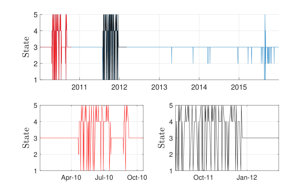 Figure 1
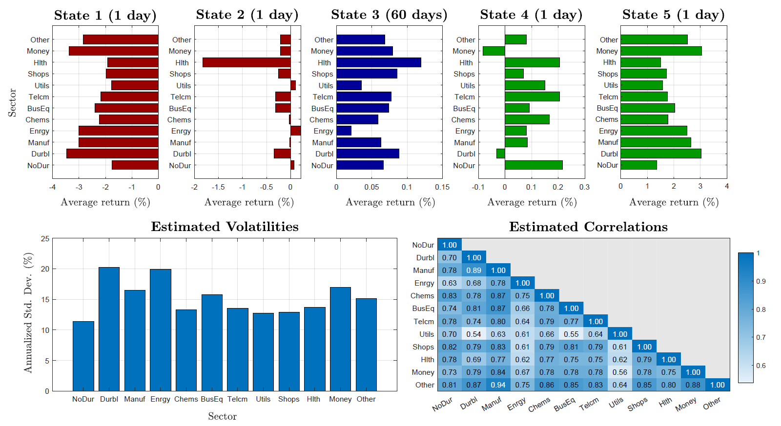 Figure 2
 Figure 3
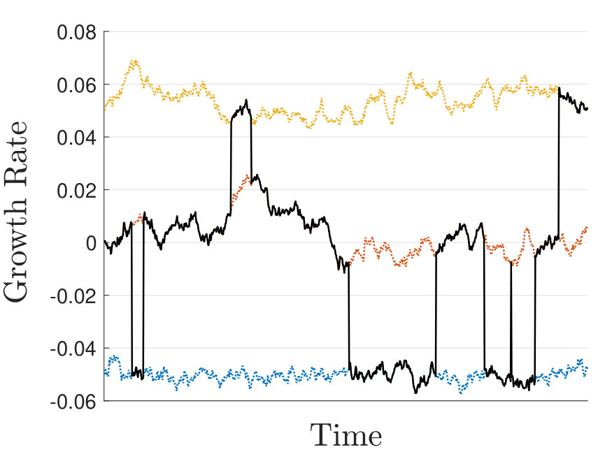 Figure 4
 Figure 5
 Figure 6
 Figure 7
 Figure 8
| Dynamic Programming | Convex Analysis | |
|---|---|---|
| Growth Rates | ||
| Bounded, deterministic, | ||
| differentiable growth rates | Stochastic, unobservable growth rates (possibly rank-dependent) | |
| Noise component | ||
| Deterministic, differentiable | ||
| volatility with Brownian noise | (or even ) martingale noise | |
| (possibly with stochastic volatility) | ||
| Benchmarks | ||
| Benchmarks are Markovian in , | ||
| differentiable maps | Benchmarks are -adapted | |
| Penalty matrices | ||
| Deterministic penalty | ||
| weighting matrices | Stochastic penalty | |
| weighting matrices | ||
| Preference parameters | ||
| Constant subjective | ||
| preference parameters | Stochastic subjective preference parameters (e.g. wealth-dependent) |
| State | Average Daily Growth Rate Across Industries | Number of Days Spent in State | % of Days Spent in State | Expected Sojourn Time |
| Very Bad | -250 bps | 44 | 3 % | 1 day |
| Bad | -25 bps | 28 | 2 % | 1 day |
| Normal | 7 bps | 1305 | 86 % | 60 days |
| Good | 10 bps | 89 | 6 % | 1 day |
| Very Good | 210 bps | 44 | 3 % | 1 day |
Peer Reviews
No public reviews on file for this paper yet. If you reviewed it on a platform where reviews are public (OpenReview, ICLR, NeurIPS, ICML), you can paste yours below so the community can read it here.
Videos
No videos yet. Explain this paper in a talk, walkthrough, or lecture? Add one.
Active and Passive Portfolio Management with Latent Factors
Ali Al-Aradi
Sebastian Jaimungal
Department of Statistical Sciences, University of Toronto
Abstract
We address a portfolio selection problem that combines active (outperformance) and passive (tracking) objectives using techniques from convex analysis. We assume a general semimartingale market model where the assets’ growth rate processes are driven by a latent factor. Using techniques from convex analysis we obtain a closed-form solution for the optimal portfolio and provide a theorem establishing its uniqueness. The motivation for incorporating latent factors is to achieve improved growth rate estimation, an otherwise notoriously difficult task. To this end, we focus on a model where growth rates are driven by an unobservable Markov chain. The solution in this case requires a filtering step to obtain posterior probabilities for the state of the Markov chain from asset price information, which are subsequently used to find the optimal allocation. We show the optimal strategy is the posterior average of the optimal strategies the investor would have held in each state assuming the Markov chain remains in that state. Finally, we implement a number of historical backtests to demonstrate the performance of the optimal portfolio.
keywords:
Active portfolio management; Convex analysis; Stochastic Portfolio Theory; Functionally generated portfolios; Rank-based models; Growth optimal portfolio; Hidden Markov models; Partial information.
t1t1footnotetext: The authors would like to thank NSERC for partially funding this work.
1 Introduction
Problems in portfolio management can be divided into two types: active and passive. In the former, investors aim to achieve superior portfolio returns; in the latter, the investors’ goal is to track a preselected index; see, for example, Buckley and Korn (1998) or Pliska and Suzuki (2004). One can further separate active portfolio management objectives into two types: absolute and relative. There is a great deal of literature dedicated to solving various portfolio selection problems with absolute goals via stochastic control theory. The seminal work of Merton (1969) introduced the dynamic asset allocation and consumption problem, utilizing stochastic control techniques to derive optimal investment and consumption policies. Extensions can be found in Merton (1971), Magill and Constantinides (1976), Davis and Norman (1990), Browne (1997) and more recently Blanchet-Scalliet et al. (2008), Liu and Muhle-Karbe (2013) and Ang et al. (2014) to name a few. The focus in these papers is generally on maximizing the utility of discounted consumption and terminal wealth or minimizing shortfall probability, or other related absolute performance measures that are independent of any external benchmark or relative goal. Works on optimal active portfolio management with relative goals (i.e. attempting to outperform a given benchmark) can be found in Browne (1999a), Browne (1999b) and Browne (2000), Pham (2003) and, more recently, Oderda (2015).
There are also several works that address the question of achieving absolute portfolio selection goals when parameters are stochastic, including cases where the investor only has access to partial information and must rely on Bayesian learning or filtering techniques to solve for their optimal allocation. Merton (1971) solves for the portfolio that maximizes expected terminal wealth assuming that the instantaneous expected rate of return follows a mean-reverting diffusive process. Lakner (1998) extends this to the case where the drift processes are unobservable. In Rieder and Bäuerle (2005) the assets’ drift switches between various quantities according to an unobservable Markov chain; Frey et al. (2012) extends this to incorporate expert opinions, in the form of signals at random discrete times, into the filtering problem by using this observable information to obtain posterior probabilities for the state of the Markov chain. Bäuerle and Rieder (2007) introduces jumps to the asset price dynamics by including Poisson random measures with unobservable intensity processes. Latent models are also central to the work of Casgrain and Jaimungal (2018b) and Casgrain and Jaimungal (2018a) in the context of algorithmic trading and mean field games.
Many of the concepts discussed in this work, particularly the notion of functionally generated portfolios (FGPs) and rank-based models, are key concepts in Stochastic Portfolio Theory (SPT) (see Fernholz (2002) and Karatzas and Fernholz (2009) for a thorough overview). SPT is a flexible framework for analyzing portfolio behavior and market structure which takes a descriptive, rather than a normative, approach to addressing these issues, and emphasizes the use of observable quantities to make its predictions and conclusions. The appeal of SPT partially lies in the fact that it relies on a minimal set of assumptions that are readily satisfied in real equity markets and that the techniques it employs construct relative arbitrage portfolios that outperform the market almost surely without the need for parameter estimation. This is primarily done through the machinery of portfolio generating functions (PGFs), which are portfolio maps that give rise to investing strategies that depend only on prevailing market weights. A discussion of the relative arbitrage properties of FGPs and related approaches to achieving outperformance vis-à-vis the market portfolio can be found in Pal and Wong (2013), Wong (2015) and Pal and Wong (2016).
Although SPT focuses on almost sure outperformance, i.e. relative arbitrage with respect to the benchmark portfolio, we deviate from this criterion in favor of maximizing the expected growth rate differential. We present two justifications for this choice. First, certain rank-based models such as the first-order models admit equivalent martingale measures over all horizons implying the non-existence of relative arbitrage opportunities. This forces the investor to select an alternative performance criterion. Secondly, Fernholz (2002) argues for the use of functionally-generated portfolios such as diversity-weighted portfolios as benchmarks for active equity portfolio management given their passive, rule-based nature and ease of implementation. However, Wong (2015) notes that under certain reasonable conditions relative arbitrage opportunities do not exist with respect to these portfolios. Therefore, once again the investor must seek a substitute for almost sure outperformance if they decide to have a performance benchmark of this sort. One SPT-inspired work that uses an expectation-based objective function is Samo and Vervuurt (2016), in which machine learning techniques are utilized to achieve outperformance in expectation by maximizing the investor’s Sharpe ratio.
Active managers often dynamically invest in markets with the goal of achieving optimal relative returns against a performance benchmark while anchoring their portfolio to a tracking benchmark (in the sense of incurring minimal active risk/tracking error). They also often have in mind additional constraints on the investor’s portfolio, e.g. penalizing large positions in certain assets or excessive volatility in the investor’s wealth. In Al-Aradi and Jaimungal (2018), the authors formulate these goals and constraints by posing a portfolio optimization problem with log-utility of relative wealth, together with running penalty terms that incorporate the investor’s constraints on tracking a benchmark and total risk. They solve the problem in closed-form using dynamic programming under the assumptions that the benchmarks are differentiable maps that are Markovian in the asset values; this encompasses the market portfolio and, more broadly, the class of (time-dependent) functionally generated portfolios.
A shortcoming of Al-Aradi and Jaimungal (2018) is that when the investor values outperformance, the optimal solution relies crucially on the asset growth rate estimates, which are assumed to be bounded, differentiable, deterministic functions of time. However, returns are notoriously difficult to estimate robustly and the deterministic assumption does not provide adequate estimates. To address this shortcoming, here, we allow for growth rates to be stochastic and be driven by latent factors. This is essential to making the strategy robust to differing market environments. Our formulation also accommodates rank-based models; such models exploit the stability of capital distribution in the market to arrive at estimates of asset growth rates based on asset ranks.
Our modeling assumption is similar to that adopted in Casgrain and Jaimungal (2018a), who study the mean-field version of an algorithmic trading problem, where assets are driven by two components: a drift term and a martingale component both of which are adapted to an unobservable filtration. The investor’s strategy, on the other hand, is restricted to be adapted to a smaller filtration; namely, the natural filtration generated by the price process.
The approach we take to solve the stochastic control problem is based on techniques from convex analysis as in Bank et al. (2017) and Casgrain and Jaimungal (2018a), however these techniques date as far back as Cvitanić and Karatzas (1992). The reason we deviate from the dynamic programming approach taken in Al-Aradi and Jaimungal (2018) centers around the difficulty of extending that approach to more general market models. Although possible, it would be a difficult task to ensure that all the additional state variables (which would include various semimartingale local times in the case of rank-based models) satisfy the conditions for a Feynman-Kac representation to the HJB equation that arises from the control problem, which is a central aspect of the proof. A number of additional (possibly restrictive) assumptions would have to be made on the market model and, as such, the approach we adopt in the current work allows for a more succinct solution to a more general problem with fewer assumptions.
2 Model Setup
2.1 Market Model
We adopt a market model that generalizes the one in Al-Aradi and Jaimungal (2018) and is a multidimensional version of the one used in Casgrain and Jaimungal (2018a). Let be a filtered probability space, where is the natural filtration generated by all processes in the model. We assume that the market consists of assets defined as follows:
Definition 1
The stock price process for asset , for all , is a positive semimartingale satisfying:
[TABLE]
where is a -adapted process representing the asset’s (total) growth rate and is a -adapted martingale with representing the asset’s noise component.
It is convenient to work with the logarithmic representation of asset dynamics:
Proposition 1
The logarithm of prices, , satisfies the stochastic differential equation:
[TABLE]
This can also be expressed in vector notation as follows:
[TABLE]
where
[TABLE]
We make the following assumption on the growth rate and noise component of asset prices:
Assumption 1
The growth rate and martingale noise processes satisfy one of the two following conditions:
- (a)
, ; 2. (b)
* and ,*
[TABLE]
In the assumption above and for denote the -norm and -norm on , respectively. Furthermore, we will make use of the shorthand notation to denote the usual Euclidean norm.
We also assume the quadratic co-variation processes associated with the noise component satisfy
Assumption 2
Let be the matrix whose -th element is the quadratic covariation process between and , . We assume that, for each , there exists and such that
[TABLE]
This is an extension of the usual non-degeneracy and bounded variance conditions.
Remark 1
The constant in of Assumption 1 may depend on the constants and that appear in Assumption 2, but provided that is sufficiently large we can ensure that the candidate optimal solution that we obtain is in fact in the set of admissible controls.
2.2 Portfolios and Observable Information
The investor does not have access to the latent processes driving asset prices and observes asset prices alone (it is possible to allow other processes in addition to the price process, but here we restrict to this case). Let the filtration where denotes the investor’s filtration.
Definition 2
A portfolio is a measurable, -adapted, vector-valued process , where such that for all , satisfies:
[TABLE]
Furthermore, we define the set of admissible portfolios as follows:
- (a)
if Assumption 1(a) is enforced, we assume and define :
[TABLE] 2. (b)
if Assumption 1(b) is enforced, we assume and define:
[TABLE]
In the sequel, we write to denote either or depending on which part of Assumption 1 is being enforced.
Remark 2
The cost of allowing for noise processes is that both growth rate processes and admissible portfolios are rather than processes.
In the definition above, portfolios are adapted to the filtration , which is the information set generated by the asset price paths and not the full information set . The latter includes the noise component as well as its quadratic covariation process , both assumed unobservable. This ensures that strategies depend only on fully observable quantities which in our context are limited to the asset price processes.
Given the model dynamics, and portfolio assumptions, we next derive the dynamics of wealth associated with an arbitrary portfolio :
Proposition 2
The logarithm of the portfolio value process satisfies the SDE:
[TABLE]
[TABLE]
and and are the portfolio growth rate and excess growth rate processes, respectively.
Proof. The proof follows the same steps as the proof of Proposition 1.1.5. of Fernholz (2002). The proportional change in the value of portfolio is a weighted average of the simple return of each asset held in the portfolio:
[TABLE]
From the asset dynamics in (2.2) and an application of Itô’s lemma we have:
[TABLE]
where is the quadratic variation process of . Another application of Itô’s lemma on the portfolio wealth process dynamics gives
[TABLE]
The result follows by noting that the quadratic variation is given by:
[TABLE]
and then rearranging terms.
2.3 Market Model Examples
Al-Aradi and Jaimungal (2018) assume growth rates and volatilities are bounded, differentiable, deterministic functions and the only driver of asset prices was a multidimensional Wiener process. In this section we present two market models satisfying the assumptions in this paper that allow for more general asset growth rates. The two models are presented with the goal of improved growth rate estimation in mind.
2.3.1 Diffusion-Switching Growth Rate Process
The diffusion-switching model assumes that asset growth rates switch between a number of possible diffusion processes according to an underlying Markov chain. That is:
[TABLE]
where is a continuous-time Markov chain with state space and is the growth rate diffusion process associated with state given as the solution to the SDE:
[TABLE]
In this formulation, is a -dimensional Wiener process driving the growth rate diffusions and and are the drift and volatility functions of the growth rate. We require and to be chosen so that for all . A sufficient set of conditions for this are the usual Lipschitz and polynomial growth conditions that guarantee the existence of a unique, square-integrable strong solution to the SDE (see Theorem 2.9 in Chapter 5 of Karatzas and Shreve (1998)). Figure 1 shows a simulation of this process when the possible diffusions are Ornstein-Uhlenbeck (OU) processes.
In Section 4, we take both and to be identically zero. This recovers the hidden Markov model (HMM) used in Rieder and Bäuerle (2005), where the growth rate switches between a number of possible constants rather than diffusion processes. This simplifies the calibration process and this is the model we employ in the implementation.
2.3.2 Second-Order Rank-Based Model
An alternative model that may be considered is the second-order rank-based model of equity markets as described in Fernholz et al. (2013). In this model, an asset’s price dynamics depend on the rank of the asset’s market weights; typically, smaller assets have higher growth rates and volatilities than larger assets. The goal of this modeling approach is to better capture observed long-term characteristics of capital distribution in equity markets, such as average rank occupation times, by exploiting the inherent stability in the capital distribution curve.
Let be the rank of asset at time , the asset price is assumed to satisfy the SDE:
[TABLE]
That is, is the “name”-based growth rate of asset and is the additional growth an asset experiences when its capitalization occupies rank . Similarly, is the volatility of the asset in rank . We assume the model parameters satisfy the requirements for the market to form an asymptotically stable system; see Fernholz et al. (2013), which also provides an outline for parameter estimation for this class of models.
It is important to notice that when this model is assumed, the rank processes for each of the stocks must be incorporated in the optimization problem as state variables. This can vastly complicate the proof of optimality when using a dynamic programming approach. The approach we take in the present work does not suffer from these issues involving local times and non-differentiability. Finally, we note that it is possible to create a hybrid model that is rank-dependent and driven by an unobservable Markov chain, but this may lead to difficulties in the parameter estimation.
3 Stochastic Control Problem
3.1 Description
The stochastic control problem we consider is similar to the one posed in Al-Aradi and Jaimungal (2018). The investor fixes two portfolios against which they measure their outperformance and their active risk, respectively. That is, the investor chooses a performance benchmark , which they wish to outperform, and a tracking benchmark , which they penalize deviations from. The objective is to determine the portfolio process that maximizes the expected growth rate differential relative to over the investment horizon . Moreover, the investor is penalized for taking on excessive levels of active risk (measured against ). An additional penalty independent of the two benchmarks is also included to control absolute risk (as measured by quadratic variation of wealth) or penalize allocation to certain assets as discussed in Section 4 of Al-Aradi and Jaimungal (2018).
The main state variable in our optimization problem is the logarithm of the ratio of the wealth of an arbitrary portfolio relative to a preselected performance benchmark . Let denote the logarithm of relative portfolio wealth for the portfolios and . Then this process satisfies the SDE:
[TABLE]
which in turn implies
[TABLE]
Our main stochastic control problem is to find the optimal portfolio which, if the supremum is attained in the set of admissible strategies, achieves
[TABLE]
where is the performance criteria of a portfolio given by:
[TABLE]
Here, is a constant and with is an -adapted process defined on for some fixed . The vector represents the subjective preference parameters set by the investors to reflect their emphasis on three goals:
The first term is a terminal reward term which corresponds to the investor wishing to maximize the expected growth rate differential between their portfolio and the performance benchmark . It is also equivalent to maximizing the expected utility of relative wealth assuming a log-utility function. 2. 2.
The second term is a running penalty term which penalizes deviations from the tracking benchmark. When , the investor is penalizing risk-weighted deviations from the tracking benchmark, with deviations in riskier assets being penalized more heavily. Thus, this can be seen as the investor aiming to minimize tracking error/active risk. 3. 3.
The final term is a general quadratic running penalty term that does not involve either benchmark. One possible choice for is the covariance matrix , which can be adopted to minimize the absolute risk of the portfolio measured in terms of the quadratic variation of the portfolio wealth process, . Another option is to let be a constant diagonal matrix, which has the effect of penalizing allocation in each asset according to the magnitude of the corresponding diagonal entry. The investor can use this choice of as a way of imposing a set of “soft” constraints on allocation to each asset.
The reader is referred to Al-Aradi and Jaimungal (2018) for further interpretation of these terms.
Remark 3
The two preference parameters can be stochastic; e.g., they may depend on the investor’s wealth level or other factors. Furthermore, the preference parameters are restricted to for two reasons: firstly, it simplifies the proof of optimality; secondly, from Al-Aradi and Jaimungal (2018), the results are driven by the relative weights, rather than absolute weights, therefore restriction to the cube results in no loss of generality.
Remark 4
The benchmarks may be non-Markovian; if they are Markovian and can be represented as and , the functions and are not restricted to be differentiable. This allows for a much wider class of benchmarks including rank-based portfolios and portfolios constructed using additional information not related to asset prices, e.g., factor portfolios based on company fundamentals. Benchmarks from the class of functionally generated portfolios are allowed, including the market portfolio, as well as portfolios generated by rank-dependent portfolio generating functions, such as large-cap portfolios.
We also require the following assumption on the relative and absolute penalty matrices and :
Assumption 3
The penalty matrices and are -adapted matrix-valued stochastic processes such that, for each , there exists constants and satisfying
[TABLE]
These bounds play an analogous role to the nondegeneracy and bounded variance assumptions made on the quadratic covariation , and ensure that the candidate optimal control we derive later is in fact admissible.
Allowing for stochastic penalty matrices is useful as it opens the door for stochastic volatility models in the case of (when choosing ) and stochastic transaction costs in the case of .
We next rewrite the control problem in terms of running reward/penalty terms. When either of the conditions in Assumption 1 is enforced, the expected value of the last integral in (3.2) is zero as the stochastic integral is in fact a martingale. Further, assuming that , the performance criteria becomes
[TABLE]
The generalizations achieved thus far compared to Al-Aradi and Jaimungal (2018) are summarized in Table 3.1 below.
The reference list from the paper itself. Each links out to its DOI / PubMed record.
- 1Al-Aradi and Jaimungal (2018) Al-Aradi, A. and S. Jaimungal (2018). Outperformance and tracking: Dynamic asset allocation for active and passive portfolio management. Applied Mathematical Finance, Forthcoming .
- 2Ang et al. (2014) Ang, A., D. Papanikolaou, and M. M. Westerfield (2014). Portfolio choice with illiquid assets. Management Science 60 (11), 2737–2761.
- 3Bank et al. (2017) Bank, P., H. M. Soner, and M. Voß (2017). Hedging with temporary price impact. Mathematics and Financial Economics 11 (2), 215–239.
- 4Bäuerle and Rieder (2007) Bäuerle, N. and U. Rieder (2007). Portfolio optimization with jumps and unobservable intensity process. Mathematical Finance 17 (2), 205–224.
- 5Baum et al. (1970) Baum, L. E., T. Petrie, G. Soules, and N. Weiss (1970). A maximization technique occurring in the statistical analysis of probabilistic functions of markov chains. The annals of mathematical statistics 41 (1), 164–171.
- 6Biernacki et al. (2000) Biernacki, C., G. Celeux, and G. Govaert (2000, July). Assessing a mixture model for clustering with the integrated completed likelihood. IEEE Trans. Pattern Anal. Mach. Intell. 22 (7), 719–725.
- 7Bishop (2006) Bishop, C. M. (2006). Pattern Recognition and Machine Learning (Information Science and Statistics) . Berlin, Heidelberg: Springer-Verlag.
- 8Blanchet-Scalliet et al. (2008) Blanchet-Scalliet, C., N. E. Karoui, M. Jeanblanc, and L. Materllini (2008). Optimal investment decisions when time-horizon is uncertain. Journal of Mathematical Economics 44 (11), 1100–1113.