TL;DR
This paper develops and tests symplectic numerical methods for guiding-center orbits in magnetic confinement devices, improving long-term accuracy and computational efficiency over traditional schemes.
Contribution
It introduces a generalized semi-implicit symplectic integration approach with coordinate transformations for plasma particle guiding-center motion.
Findings
Symplectic methods outperform adaptive Runge-Kutta in long-term orbit simulations.
The new approach achieves over three times speed-up in particle loss statistics.
Coordinate transformations enable efficient parallel computations in complex magnetic fields.
Abstract
We study symplectic numerical integration of mechanical systems with a Hamiltonian specified in non-canonical coordinates and its application to guiding-center motion of charged plasma particles in magnetic confinement devices. The technique combines time-stepping in canonical coordinates with quadrature in non-canonical coordinates and is applicable in systems where a global transformation to canonical coordinates is known but its inverse is not. A fully implicit class of symplectic Runge-Kutta schemes has recently been introduced and applied to guiding-center motion by [Zhang et al., Phys. Plasmas 21, 32504 (2014)]. Here a generalization of this approach with emphasis on semi-implicit partitioned schemes is described together with methods to enhance their performance, in particular avoiding evaluation of non-canonical variables at full time steps. For application in toroidal plasma…
Click any figure to enlarge with its caption.
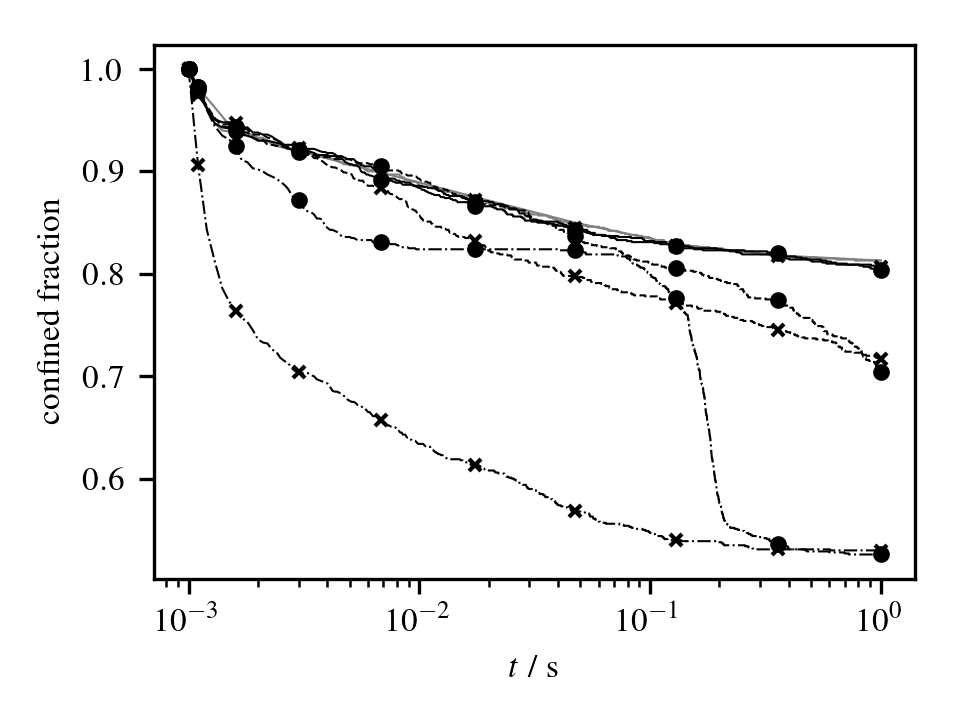 Figure 1
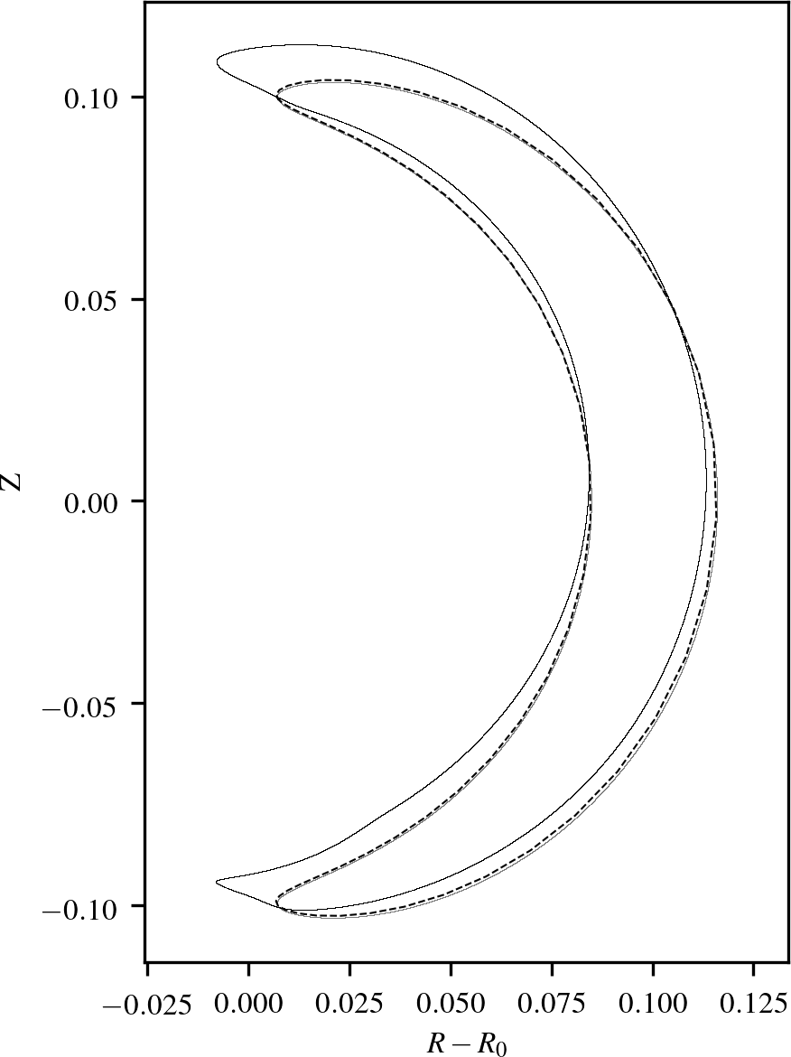 Figure 2
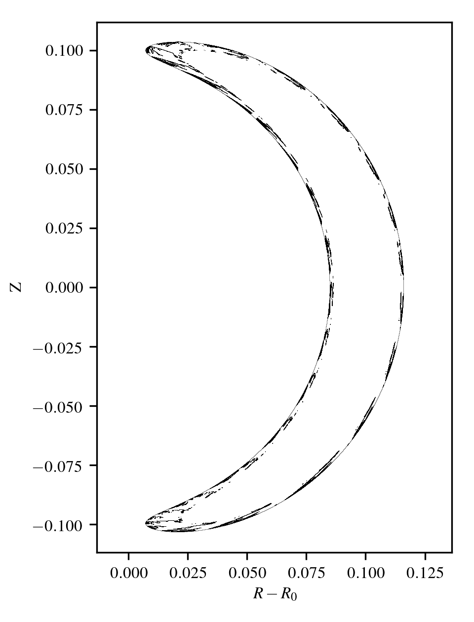 Figure 3
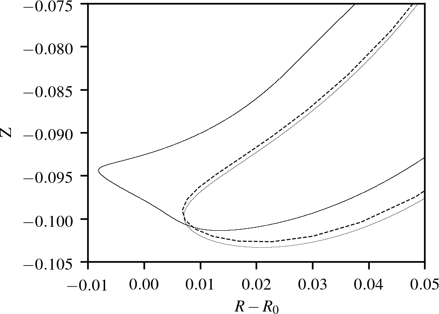 Figure 4
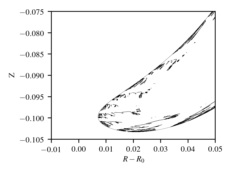 Figure 5
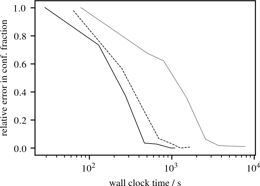 Figure 6
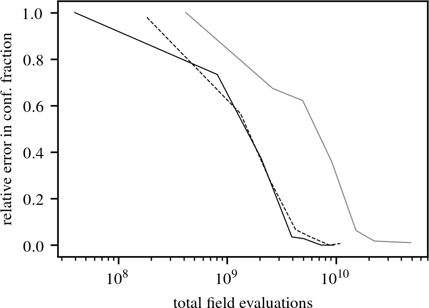 Figure 7
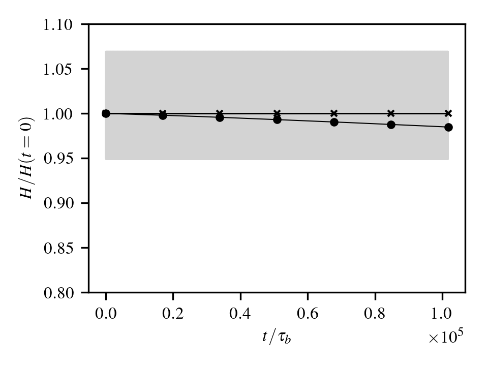 Figure 8
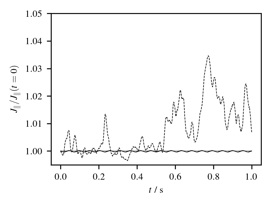 Figure 9
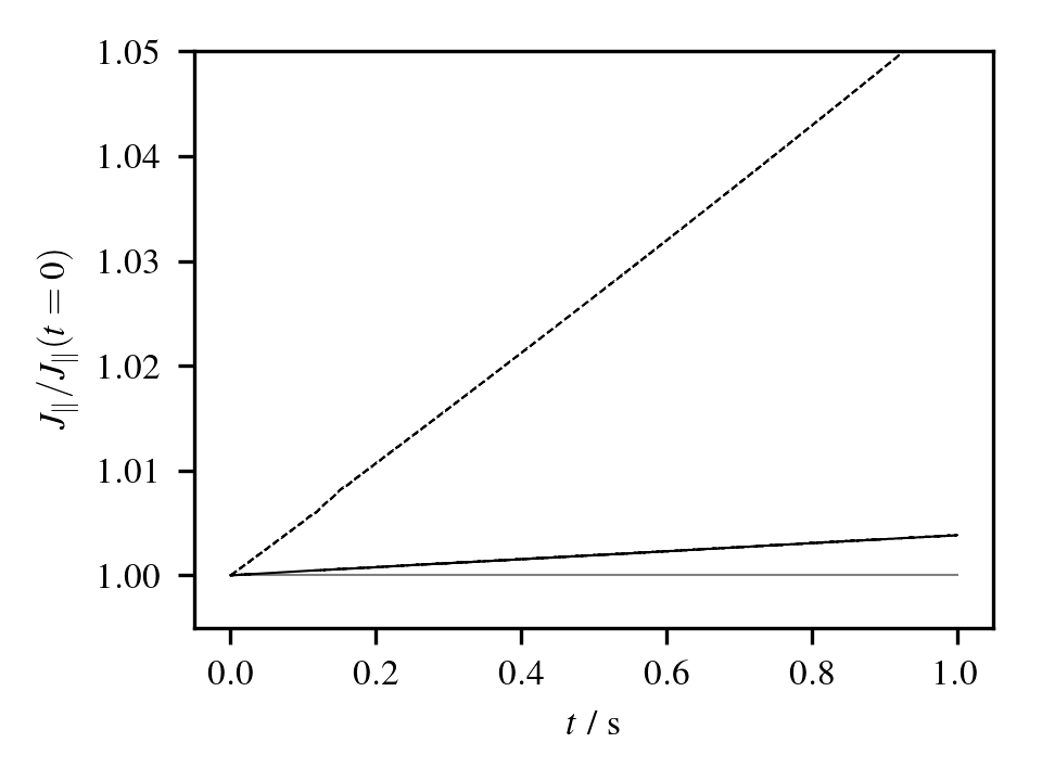 Figure 10
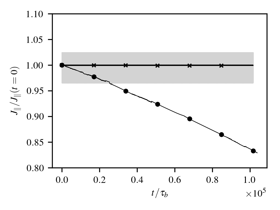 Figure 11
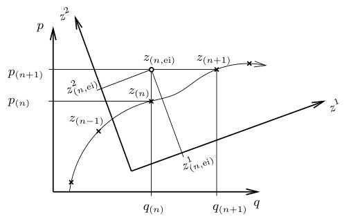 Figure 12
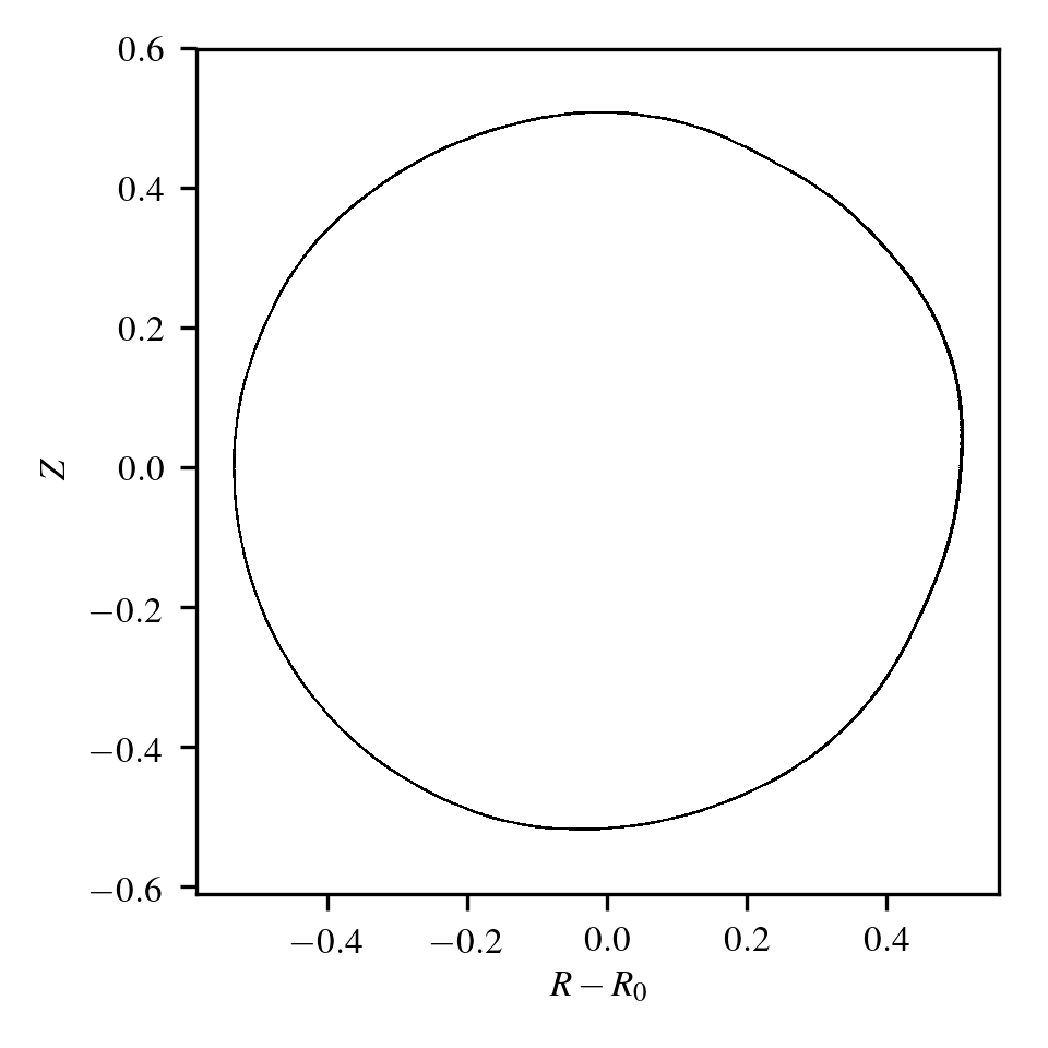 Figure 13
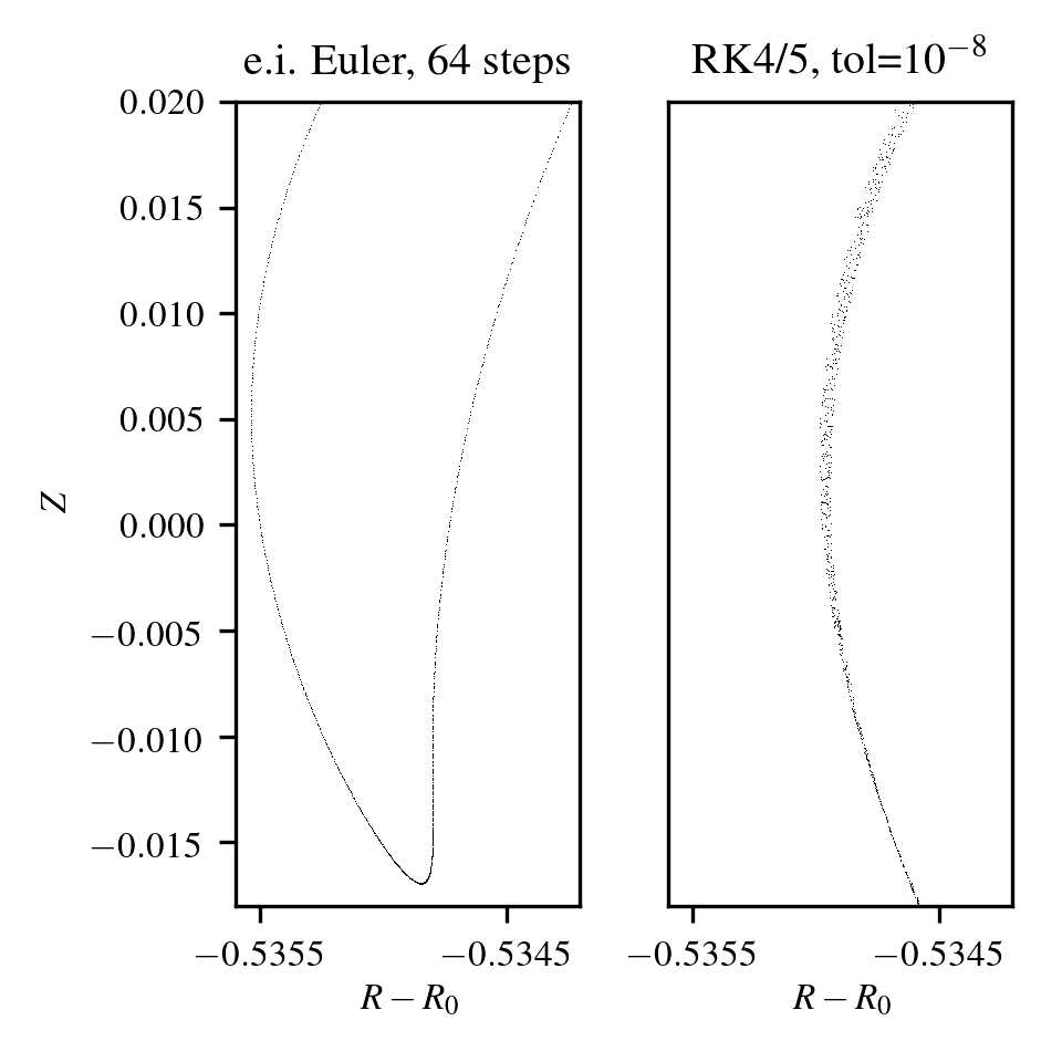 Figure 14
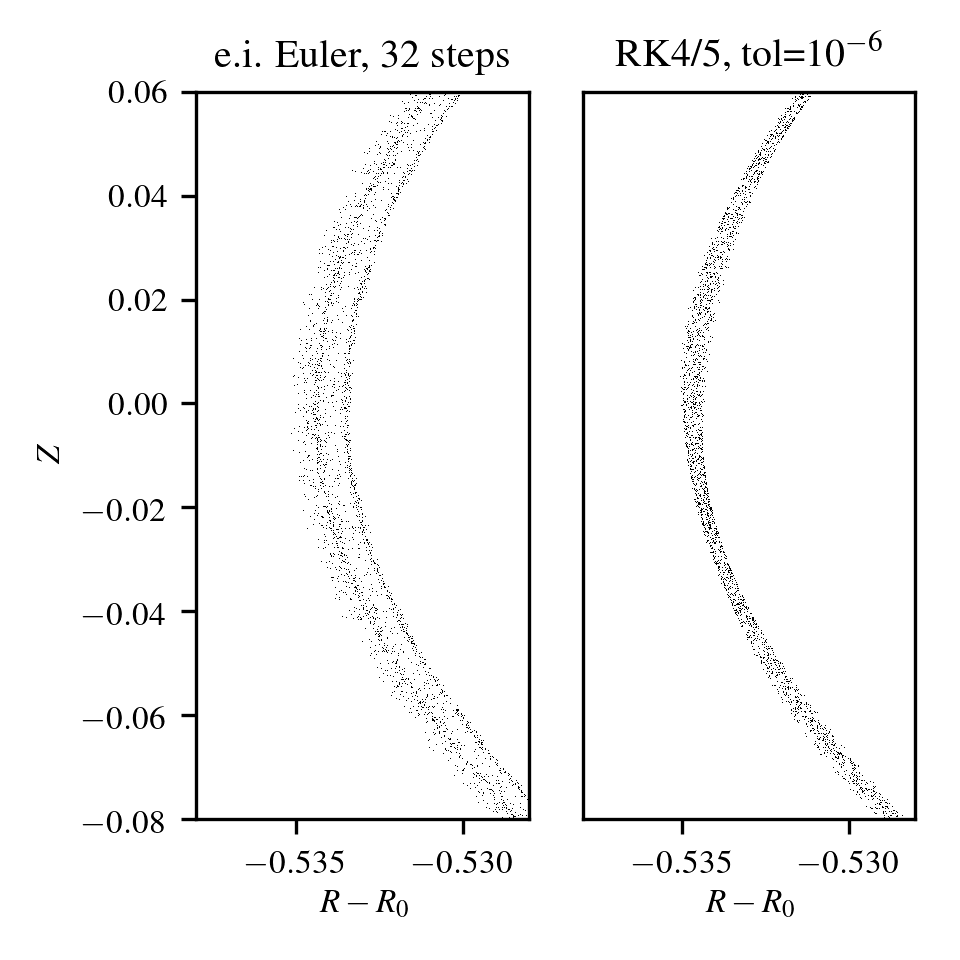 Figure 15
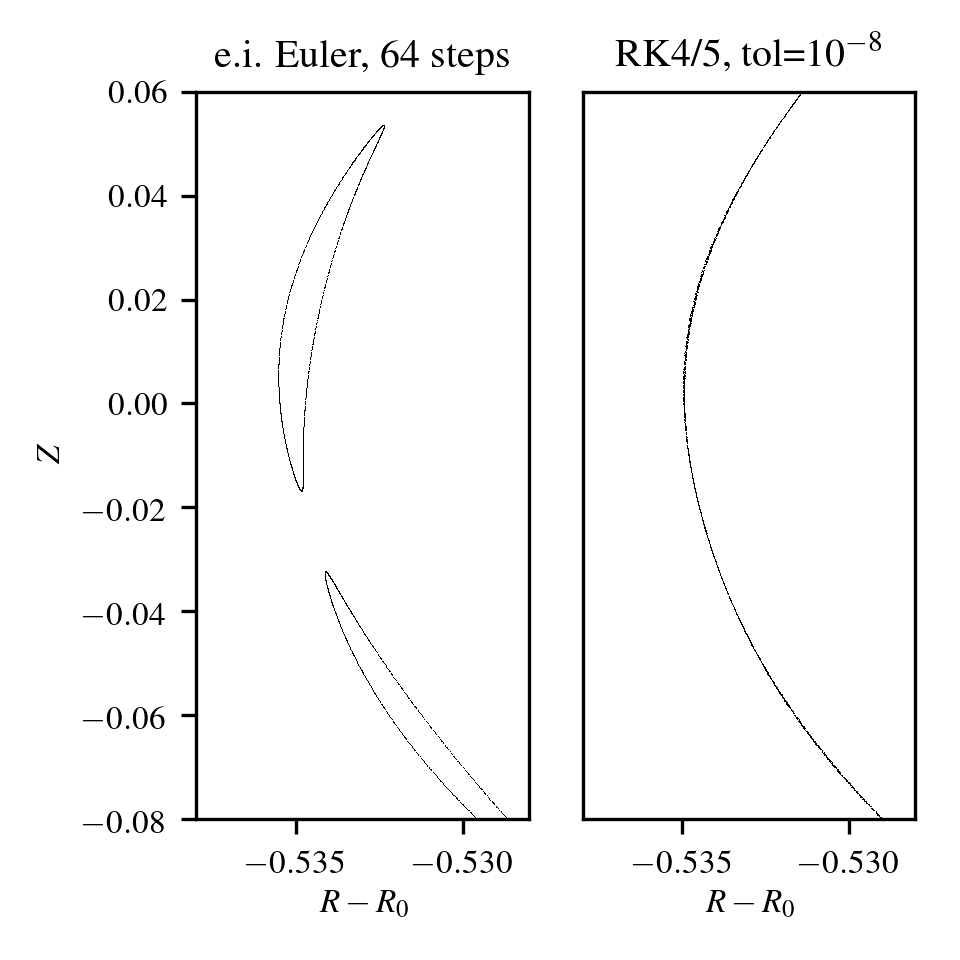 Figure 16
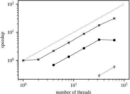 Figure 17
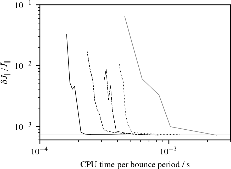 Figure 18
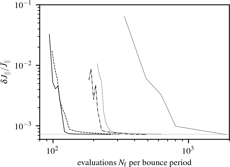 Figure 19
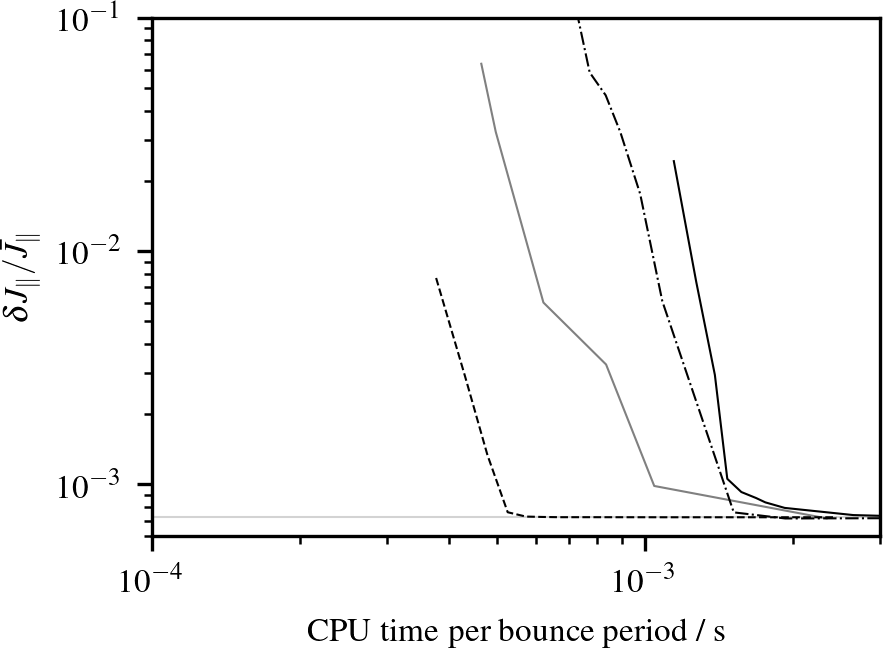 Figure 20
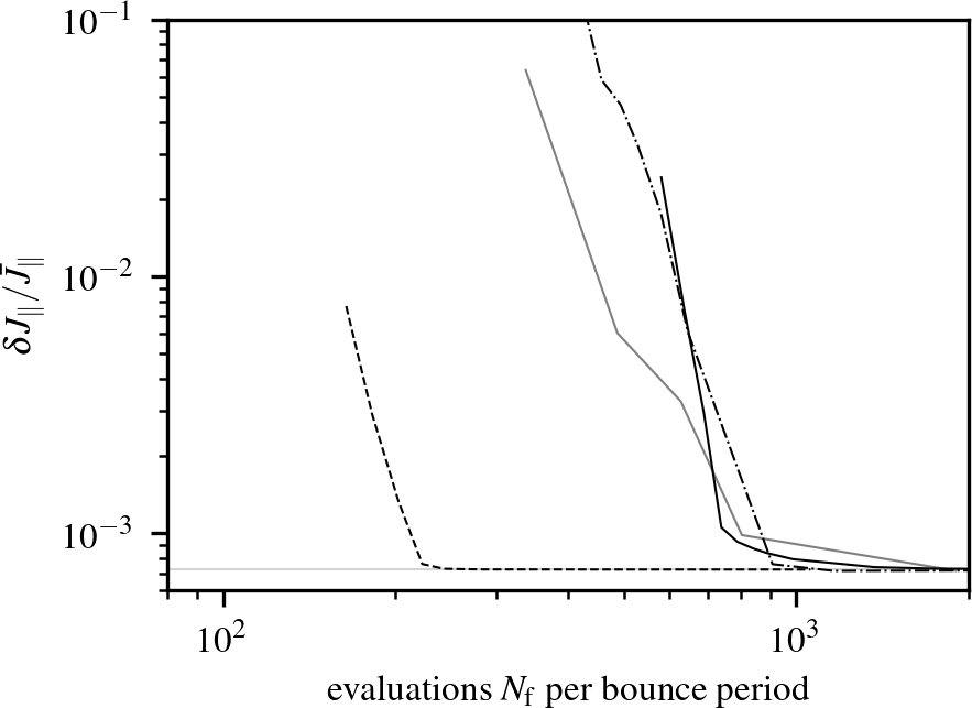 Figure 21
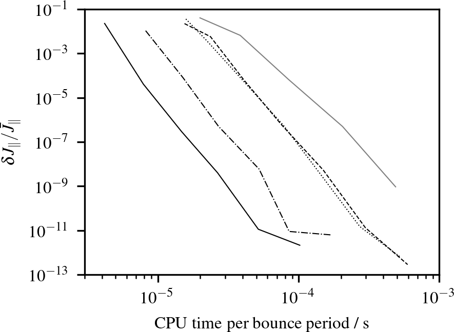 Figure 22
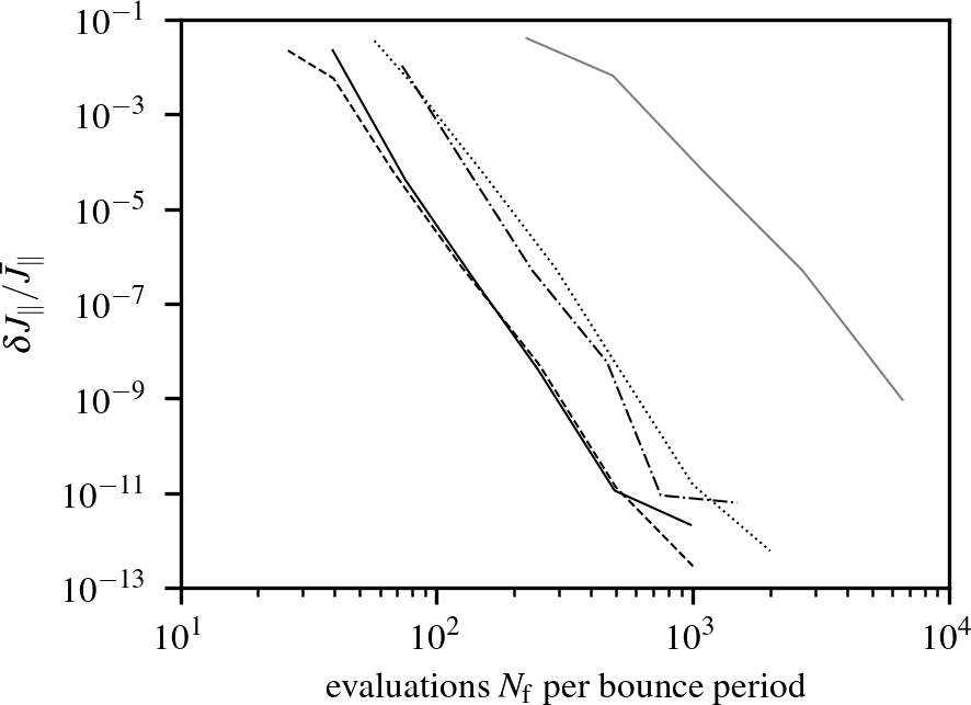 Figure 23
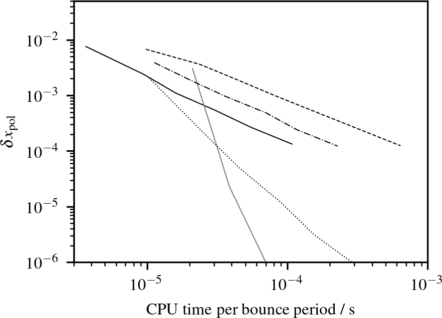 Figure 24
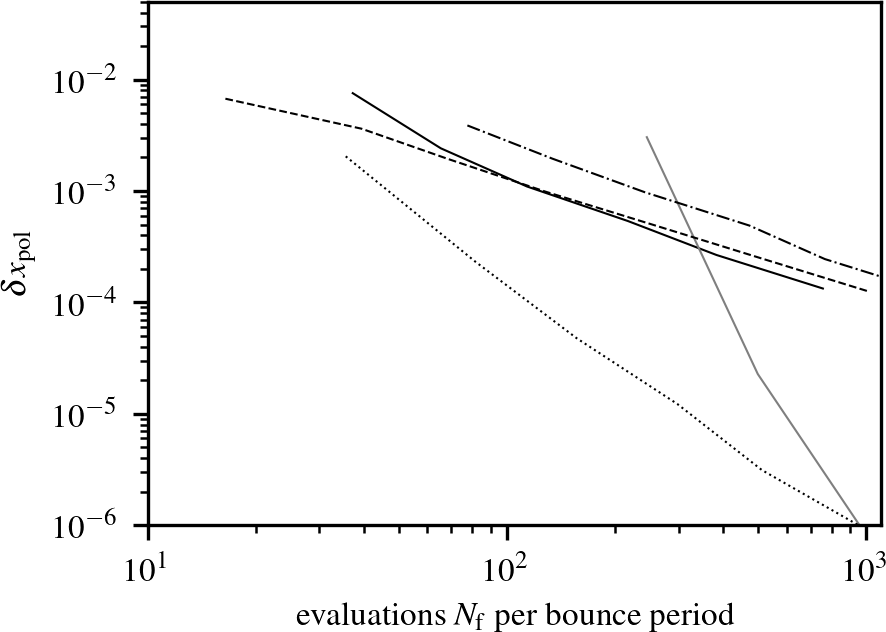 Figure 25
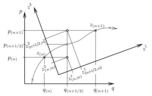 Figure 26
Peer Reviews
No public reviews on file for this paper yet. If you reviewed it on a platform where reviews are public (OpenReview, ICLR, NeurIPS, ICML), you can paste yours below so the community can read it here.
Code & Models
Videos
No videos yet. Explain this paper in a talk, walkthrough, or lecture? Add one.
Symplectic integration with non-canonical quadrature for guiding-center
orbits in magnetic confinement devices
Christopher G. Albert1, Sergei V. Kasilov2,3, Winfried Kernbichler2
1Max-Planck-Institut für Plasmaphysik, Boltzmannstraße 2, 85748 Garching, Germany
2Fusion@ÖAW, Institute of Theoretical and Computational Physics, Graz University of Technology, Petersgasse 16, 8010 Graz, Austria
3Institute of Plasma Physics, National Science Center “Kharkov Institute of Physics and Technology”,
Akademicheskaya Str. 1, 61108 Kharkov, Ukraine
(March 2, 2024)
Abstract
We study symplectic numerical integration of mechanical systems with a Hamiltonian specified in non-canonical coordinates and its application to guiding-center motion of charged plasma particles in magnetic confinement devices. The technique combines time-stepping in canonical coordinates with quadrature in non-canonical coordinates and is applicable in systems where a global transformation to canonical coordinates is known but its inverse is not. A fully implicit class of symplectic Runge-Kutta schemes has recently been introduced and applied to guiding-center motion by [Zhang et al., Phys. Plasmas 21, 32504 (2014)]. Here a generalization of this approach with emphasis on semi-implicit partitioned schemes is described together with methods to enhance their performance, in particular avoiding evaluation of non-canonical variables at full time steps. For application in toroidal plasma confinement configurations with nested magnetic flux surfaces a global canonicalization of coordinates for the guiding-center Lagrangian by a spatial transform is presented that allows for pre-computation of the required map in a parallel algorithm in the case of time-independent magnetic field geometry. Guiding-center orbits are studied in stationary magnetic equilibrium fields of an axisymmetric tokamak and a realistic three-dimensional stellarator configuration. Superior long-term properties of symplectic methods are demonstrated in comparison to a conventional adaptive Runge-Kutta scheme. Finally statistics of fast fusion alpha particle losses over their slowing-down time are computed in the stellarator field on a representative sample, reaching a speed-up of the symplectic Euler scheme by more than a factor three compared to usual Runge-Kutta schemes while keeping the same statistical accuracy and linear scaling with the number of computing threads.
1 Introduction
Symplectic integrators [1, 2] preserve the structure of Hamiltonian systems in their discretized form for numerical treatment. Apart from advantages for theoretical analysis of such methods a major practical feature of symplectic integrators is long-term stability at relatively large timesteps and good approximate conservation of integrals of motion. Symplectic integrators rely on canonical coordinates which allow for integration schemes that are easy to implement, ranging from the lowest order explicit-implicit Euler method to Gauss-Legendre and Lobatto quadrature of arbitrary high order. Applications of classical symplectic integrators include long-term tracing of charged particle orbits in electromagnetic fields of particle accelerators [3] and in plasmas [4]. Application to systems with a non-canonical formulation such as motion of guiding-centers instead of particles, require additional modifications. Existing methods often rely on explicit expressions to obtain non-canonical coordinates in terms of canonical ones in simplified geometry [5, 6, 7]. An internal report [8] not published until recently already mentions the idea of including transformation equations in an implicit way that is pursued here. Recently a general way to construct fully implicit non-canonical symplectic integrators has been applied using symplectic Runge-Kutta schemes [9, 10]. The way an integrator is constructed there is based on a construction of a transformation from non-canonical phase-space coordinates to canonical ones which is always possible at least locally according to the Darboux-Lie theorem. More generally such integrators form a special class of Poisson integrators based on this theorem, described in Ref. [1], pp. 241-242 where the idea of the present approach is already outlined but realized only for explicit inverse transformations from canonical to non-canonical coordinates. The key observation of Refs. [8] and [9] used here is that for a (semi-)implicit integrator it is enough to know this inverse implicitly. Here we limit ourselves to the case where global canonical coordinates exist which is realized for the intended application to guiding-center motion in toroidal fusion devices with nested magnetic flux surfaces.
Consider a mechanical system with Hamiltonian and Poisson brackets given in non-canonical coordinates with a known time-independent transformation to canonical coordinates . In a numerical scheme it is possible to solve canonical equations of motion with non-canonical quadrature points that transform to the quadrature points from a symplectic method in canonical coordinates. This involves a root-finding process in order to solve the non-linear set of coordinate transformation equations in each timestep. It does however not require the construction of an inverse transformation and its interpolation in phase-space. As no further approximations are made, all features of usual symplectic integrators are retained up to computer accuracy. An interesting property of such an integrator is that in general the quadrature points for follow implicitly from the restriction that the method remains symplectic in the canonical sense in each timestep, which is guaranteed by fixed quadrature points for . The result of this approach is a special class of multistage methods with internal stages in non-canonical and with canonical kept at full steps. Variants of Gauss-Legendre quadrature such as the implicit midpoint rule used in [9] are a particular case where non-canonical link and at the same point in time. Loosening this requirement makes it possible to formulate semi-implicit and partitioned rather than fully implicit integrators that share their favorable long-term properties and optionally allow to reconstruct values of at full steps if needed.
In the guiding-center formulation [11, 12, 13, 14] the fast gyration scale of charged particles in a strong magnetic field is removed by a coordinate transformation in phase-space, effectively reducing the number of degrees of freedom by one, where the gyrophase appears as a cyclic variable. Rather than looking at the particle position, one is interested in the position of the guiding-center, around which the particle gyrates periodically. In addition to three coordinates of the guiding-center, the ignorable gyrophase remains as a fourth position-like coordinate, leaving only two momentum- or velocity-like coordinates to parametrize six-dimensional phase space. This imbalance makes it immediately clear that such a description must be non-canonical. Until recently the only available structure-preserving integrators for guiding-center motion in general magnetic field geometry were variational integrators based on discretization of the action principle with the guiding-center Lagrangian in non-canonical coordinates [15, 16]. As this Lagrangian is degenerate, i.e. doesn’t contain kinetic energy as a positive-definite quadratic form on velocities, variational guiding-center integrators are prone to multistep parasitic mode instabilities. This has only recently been resolved by using degenerate variational integrators or projected variational integrators [17, 18, 19, 20]. Another way to approximately or exactly conserve invariants is possible via a geometric integrator based on a partition of space into a mesh [21, 22]. Due to low order interpolation, depending on the symmetry of the mesh, such integrators can introduce an intolerable amount of artificial stochasticity when used in non-axisymmetric configurations. Alternative approaches based on symplectic integration in the classical sense are thus still of interest.
An important result underlying the construction of symplectic integrators for guiding-center motion is the possibility to construct a transformation that restores a canonical form of the guiding-center Lagrangian [23, 24, 9, 25, 17], making canonical momenta available as functions of non-canonical phase-space coordinates. For magnetic configurations with nested flux-surfaces a purely spatial transformation can be pre-computed globally in a parallel manner. After that, symplectic integration of an arbitrary number of orbits in non-canonical coordinates is possible without additional computational overhead from the canonicalization.
The constructed integrators conserve total energy and parallel adiabatic invariant within fixed bounds and exactly conserve angular momentum in axisymmetric configurations. This makes them suitable for tracing orbits in low-collisional plasma regimes over a long period of time, including thermal ions in plasma at reactor-relevant conditions as well as fast fusion particles especially important for stellarator optimization [26, 27, 28, 29, 30]. For practical applications a reduction in computation time compared to usual Runge-Kutta methods is necessary. In this respect we first discuss the general form and features of the described integrators in section 2 with some optimizations to make them competitive with existing methods in terms of computing time. Then we proceed to the application to guiding-center motion, describing canonicalization of coordinates in section 3 and construction of integrators in section 4. In section 5 results are presented and discussed, and a final summary is given in section 6.
Notation
Here we fix some notational conventions for the following text. Letters are used for spatial coordinates, for canonical coordinates and for generally non-canonical coordinates in phase-space. Lower index notation for canonical momenta is used since in the classical construction are not only coordinates in phase-space but also components of covectors with respect to configuration space charted by coordinates . Latin indices run from to for spatial coordinates , over the number of internal stages if used for an integration scheme, or from to for canonical coordinates in a system with degrees of freedom. The index is reserved for notation of time-steps. Greek indices like are used for general phase-space coordinates and run from to . We use the usual convention from tensor algebra to sum over indices appearing once up and once down in formulas, i.e. , where indexes in the denominator of derivatives switch their position, e.g. has a lower index. Coordinate tuples are denoted by bold upright letters , while vectors, covectors and tensors use italic bold letters . We use the convention to denote functional dependencies such as by the same letters as alone, as often used in physics literature. If arguments are not written explicitly inside functions the meaning should become clear from the respective context. Explicit time dependencies of fields, Lagrangian and Hamiltonian are always suppressed, but the general results of this work remain valid also in explicitly time-dependent systems. A notable exception is the transition map from non-canonical to canonical coordinates that must remain fixed over the integration time. For guiding-center orbits this limits the application to fixed or slowly evolving magnetic configurations but permits a time-dependent electrostatic potential.
2 Symplectic integrators with non-canonical quadrature points
Motivated from the problem of guiding-center motion our goal is to find symplectic numerical methods for a dynamical system in -dimensional phase-space of a mechanical system with degrees of freedom and dynamics specified by a Hamiltonian and Poisson brackets (or a symplectic structure ). Phase-points are charted in terms of tuples of non-canonical coordinates via a coordinate chart map . A phase-point is a coordinate-independent quantity and not identified with the tuple whose values depend on the chosen coordinate system if is fixed. An explicit expression of the Hamiltonian shall exist only in non-canonical coordinates . In addition a transition map i.e. a coordinate transformation from to canonical coordinates valid in the phase-space domain of interest shall be given by explicit and invertible functions
[TABLE]
with inverses given only implicitly.
Equations of motion for the evolution of can be written in terms of via
[TABLE]
Derivatives of over are evaluated as elements of the inverse Jacobian matrix of Eq. (1),
[TABLE]
leaving only dependencies on on the right-hand side of Eqs. (2-3). Based on an existing symplectic numerical integration scheme in discrete equivalents of the equations (2-3) augmented by constraints (1) are solved implicitly in variables via a root-finding method in each timestep. Quadrature points of a chosen symplectic method for canonical variables fix the respective evaluation point in phase-space. Quadrature points of non-canonical variables follow implicitly by the fact that they should describe the same point in phase-space via the equations (1) solved for and up to machine accuracy. The resulting virtual connect positions and momenta at possibly different times , but for the same phase-point . The details of this procedure will be illustrated in the following section for different numerical schemes. Evaluation of the Hamiltonian at a point in phase-space fixed by a symplectic scheme in canonical coordinates guarantees symplecticity of the integration scheme despite evaluation in terms of non-canonical coordinates . An explicit proof of symplecticity for a particular scheme can easily be stated by using the chain rule inside a standard proof [1, 2] to express either the co- or contravariant representation of the canonical two-form in terms of non-canonical coordinates.
2.1 Semi-implicit schemes of first order
The explicit-implicit Euler scheme
Starting at the lowest order we consider the symplectic explicit-implicit Euler scheme with time-step in canonical coordinates given by
[TABLE]
Here all position coordinates are evaluated explicitly at the current time at the -th step, and all momentum coordinates are evaluated implicitly at the subsequent step . We now modify the scheme in terms of non-canonical quadrature points that have to describe a phase point that is charted by canonical coordinates with Eqs. (1) being fulfilled. Quadrature points for non-canonical with this property are not known a priori, and not necessarily all correspond to coordinate values realized by the actual orbit at any given time. To reflect this, we use subscript “ei” marking the explicit-implicit quadrature scheme to denote the phase-point described by canonical coordinate values as well as its non-canonical coordinate values . The scheme is illustrated in Fig. 1 for configuration space dimension .
For the implicit step (5), formally equations have to be solved in variables :
[TABLE]
where is evaluated in and we have used the short-hand notation
[TABLE]
for the pertinent element of the inverse Jacobian matrix (4) of the coordinate transform (1). We can eliminate equations in (8) right away if we replace in Eq. (9) by the function and store the result for the subsequent timestep on evaluation. The final set of implicit equation to solve in is
[TABLE]
Since non-canonical are uniquely linked to a phase-point with canonical coordinates the problem is well-posed and has a unique solution in within the stability bounds of for the underlying symplectic scheme in . After solving Eqs. (11-12), new canonical position values are explicitly given via (6),
[TABLE]
The implicit-explicit Euler scheme
The implicit-explicit Euler scheme is the adjoint to the explicit-implicit scheme, i.e. the schemes transform into each other under time-reversal. In the implicit-explicit Euler scheme quadrature points of and are swapped compared to the explicit-implicit Euler scheme and the implicit system to solve in (“ie” for “implicit-explicit”) becomes
[TABLE]
After finding a sufficiently converged solution to Eqs. (14-15) we explicitly evaluate
[TABLE]
2.2 Higher order schemes
Despite their symplectic property, the accuracy of the two partitioned Euler schemes suffers from their low order and their time-asymmetry, leading to significant distortion of phase-space when large time-steps are used [1]. For applications where this behavior must be avoided the self-adjoint/time-reversible second-order Verlet (leapfrog) algorithm can be used. It is constructed as a combination of the two partitioned Euler schemes in the following way (Fig. 2).
Perform an implicit-explicit Euler step replacing by , and by . The solution of Eqs. (14-15) yields intermediate non-canonical variables and midpoint positions . Midpoint momenta follow via (16). 2. 2.
Perform an explicit-implicit Euler step replacing by , and by . The solution of Eqs. (11-12) yields intermediate non-canonical variables replacing with new momenta and finally new positions via Eq. (13).
The described semi-implicit symplectic Euler and Verlet methods are partitioned into implicit and explicit steps. Also the fully implicit second-order midpoint rule used in [9] can be formulated in the way described above via non-canonical midpoint variables and full step variables at the next timestep,
[TABLE]
Here derviatives are evaluated at the internal stage with non-canonical coordinates . By using , , and eliminating one obtains the form
[TABLE]
described in Eq. (41) of Ref. [9], where variables in the reference correspond to our . It should be noted that the present treatment is more general than the one of Ref. [9] in the sense that it doesn’t assume canonical and non-canonical quadrature points to coincide at the same point in time to first order in each internal stage. Therefore it is applicable also to partitioned Runge-Kutta methods including the symplectic Euler and Verlet schemes described above. This makes a generalization to higher order schemes via Lobatto IIIA-IIIB pairs as well as composition of first order schemes possible in addition to Gauss-Legendre quadrature (midpoint for order 2). A symplectic partitioned Runge-Kutta integrator [1] with non-canonical quadrature points is generally given by
[TABLE]
with (no summation over , ) to guarantee symplecticity of the scheme evaluated in the phase-point . Here each component of non-canonical coordinates is evaluated independently at a virtual stage such that Eqs. (25-28) are fulfilled, without reference to time . If only approximate values for are required it is sufficient to use internal stages that are accurate at a usually reduced order. This observation is also relevant to non-partitioned schemes with . Also there it is not necessary to solve full steps in non-canonical variables. The most gain is possible in the implicit midpoint rule where Eqs. (21-22) are replaced by
[TABLE]
and the remaining equations (23-24) corresponding to Eqs. (27-28) become explicit with
[TABLE]
With this modification the dimension of the implicit system to solve is the same for both first-order Euler variants and the single-stage but second-order implicit midpoint rule for general non-canonical coordinates. As we will see in section 4.2 the choice of partly canonical variables can reduce the dimension of symplectic Euler methods, thereby producing truly semi-implicit schemes.
In case accurate results for non-canonical variables are required at full steps, the additional implicit equations
[TABLE]
have to be solved after having obtained in the time-step, thereby reducing performance. To avoid this additional overhead one can instead apply a Taylor expansion of sufficiently high order to approximate as described in A in a post-processing step.
2.3 Numerical solution of implicit equations
Iterative root-finding schemes and predictor
For finding roots of implicit sub-steps such as Eq. (9) usual Newton iterations or similar methods with superconvergence are well-suited. For the purpose of keeping the method symplectic, convergence criteria should use tolerance settings close to machine accuracy, i.e. double-precision floating point values. To retain performance comparable to explicit methods the number of iterations should be as low as possible. To achieve this, a good starting guess is required in order to initialize the root-finding algorithm. We compute an approximate initial guess for the -th internal stage via a predictor step. A common way of doing this would consist in a low-order method such as a forward Euler scheme based on the coordinate values of the previous full timestep via
[TABLE]
Here the time evolution via Poisson brackets,
[TABLE]
would be used with derivatives evaluated at via the relation of Jacobian matrices in Eq. (4). The disadvantage of forward predictor steps of this kind and especially of their higher order equivalents lies in the required extra evaluations of derivatives of and . An alternative predictor scheme that has proven to be more efficient in practice relies on polynomial extrapolation of existing data from multiple previous timesteps. The use of Lagrange polynomials for this purpose just adds negligible overhead in terms of performance and storage and doesn’t require extra evaluations of fields and derivatives such as a low-order time-stepping scheme. A starting guess for stages can either be obtained in the same manner, or by inserting the guess for into the transformation (1) to canonical coordinates.
Evaluation of fields in the numerical root
In iterative schemes the fields and are usually not evaluated in the converged solution, but only in the last iteration step before convergence has been reached. For example in the explicit-implicit Euler scheme we first find the solution to (11-12) implicitly in the final iteration, but have evaluated fields in only in the previous iteration. In Eq. (13) we however require evaluation at the converged values . In general, to obtain field values evaluated at a converged tuple of non-canonical internal stages one can avoid an extra evaluation of fields using a Taylor expansion around . Namely, one can express a function up to first order in differences from the converged solution as
[TABLE]
with evaluated at and summation over . Here is of the order of the tolerance setting in the iterative scheme. For expressions such as we require second derivatives that can be reused from the Jacobian matrix of the implicit set of equations solved by the root-finding scheme (not to be confused with the Jacobian matrix of the transformation to canonical coordinates). Within a classical (not quasi-) Newton scheme this Jacobian matrix is available from explicit computations. For practical cases where just a few iterations are needed, saving one extra evaluation increases performance considerably.
Any implicit method can only be symplectic up to the tolerance in the numerical root finding scheme. With the residual term of that order the error amplification in Eq. (37) in the linear term depends on the second factor . In particular, for guiding-center orbits in an electromagnetic field this means second spatial derivatives of Hamiltonian and poloidal momentum , respectively, governed by curvature of fields. The condition for the validity of the guiding-center approximation imposes a natural limit for their magnitude. In the practical results shown below accuracy with and without using Eq. (37) is identical at a relative tolerance of for Newton iterations.
3 Canonical form of the guiding-center Lagrangian
The fast gyro-motion of charged particles in a magnetized plasma is commonly written in terms of the guiding-center Lagrangian [11, 12, 13, 14] using non-canonical coordinates in phase space. Here coordinates parametrize the spatial position of the guiding-center for which we use the notation with one radial coordinate and two angular coordinates following [24]. This describes the important case of flux coordinates for toroidal fields with embedded closed magnetic surfaces where a global transformation to canonical coordinates is possible. In the general case for a transformation constructed only locally, any coordinate triple may be chosen instead. The pair describes gyrophase and magnetic moment and can be dropped in the full guiding center Lagrangian, as the guiding-center transformation is made such that becomes an ignorable variable and becomes a constant of motion. The last coordinate is often chosen to be the variable , corresponding to the velocity parallel to the magnetic field within leading order of the expansion. When leaving as a general coordinate, is a function of phase-space coordinates . The 4-dimensional phase-space relevant for single-particle guiding-center motion is thus a subspace of the original -dimensional phase-space, containing points charted by . It is common to introduce an effective vector potential with covariant components
[TABLE]
where are the covariant components of the unit vector along the magnetic field, is the vector potential, and and are particle mass, charge and speed of light, respectively. The modified vector potential depends on all components of , as does the Hamiltonian
[TABLE]
Fields and electrostatic potential are functions of the guiding-center position , but not of . In principle quantities can include explicit time dependencies which we do not specify in the notation. Dropping the ignorable variable and treating as a constant, the guiding-center Lagrangian describing the evolution of 4-dimensional phase space coordinates over time is given in a non-canonical form,
[TABLE]
The three terms are not canonical momenta despite their apparent similarity, since only two momenta exist in a four-dimensional phase space. This asymmetry is a usual property of the phase space Lagrangian formalism allowing for general, non-canonical phase space variable transformations which have been employed, in particular, in [11].
3.1 Transformation to canonical form
Finding a canonical form of the guiding-center Lagrangian (40) is possible [23, 24, 25, 17, 31] while keeping partially non-canonical coordinates. This is usually achieved by transforming to new phase-space coordinates with the constraint that covariant vanish identically. The canonical form of the guiding-center Lagrangian without dependency on follows as
[TABLE]
In this form the coordinates and appear directly as canonical position coordinates. The remaining part of the transition map (1) from to the two canonical momenta conjugate to and is directly identified in the canonical guiding-center Lagrangian (41) with
[TABLE]
Keeping these relations implicit for the construction of a symplectic scheme in non-canonical coordinates as described in section 2 avoids finding an inverse that would be required for a usual symplectic integrator in canonical coordinates.
Canonicalization of phase space coordinates is not unique. It can be done mixing up spatial guiding center positions with other, “velocity space” variables [23, 17, 31, 9] or transforming only the spatial coordinates [24, 25]. In the latter case we can keep and denote the angular variables of canonical coordinates as and . In the next subsection we construct such a straight field line coordinate system similar to the one introduced in Ref. [25] for tokamaks but with a different method similar to Ref. [24] which is more efficient, especially for 3D toroidal field configurations (stellarators) being of interest here. Note that in contrast to Ref. [24] which results in a non-straight field line canonical coordinate system the present method produces straight field line canonical coordinates and requires no special treatment in case turns to zero which occurs in stellarator vacuum fields. In case of axisymmetric geometry results are the same as those of Ref. [25].
3.2 Canonical straight field line flux coordinates for 3D toroidal geometry
Let original coordinates be some general straight field line magnetic flux coordinates with and with vector potential gauge , such that
[TABLE]
These coordinates are linked to any other straight field line flux coordinates (canonicalized coordinates in our case) by the transformation (see, e.g., Ref. [32])
[TABLE]
Here, is the rotational transform and is a single valued function (i.e. periodic in angles) which defines the transformation. Note that it is the inverse coordinate transformation, , which is constructed here, similarly to Ref. [24], in contrast to Ref. [25] where a direct transformation has been looked for. Covariant components of the vector potential transform by tensor algebra rules and we require to keep the gauge (here and below various vector components are marked with “c” for canonical coordinates). This means simply that the last term containing appearing in direct substitution of Eq. (45) into (44),
[TABLE]
must be dropped. Here the definition of via derivatives of the vector potential, , has been used. Thus covariant components of corresponding to magnetic fluxes remain the same also for canonical coordinates, i.e. and . An equation for the transformation function leading to , which together with annihilates the radial component of the effective vector potential (38) follows from the transformation of the covariant magnetic field components
[TABLE]
Using in the Jacobian matrix , the explicit form of the coordinate transformation given by and Eqs. (45) the condition results in the following nonlinear ordinary differential equation for ,
[TABLE]
Here and below, for one should use its explicit form (45) containing , and . In turn, the angular components of (47) define covariant angular canonical components of the magnetic field via and its angular derivatives explicitly,
[TABLE]
The metric determinant of the canonical flux coordinates is also explicitly defined via , its derivatives and the metric determinant of the original flux coordinates as follows,
[TABLE]
This yields explicit expressions for the contra-variant field components,
[TABLE]
and, therefore, completes the definition of the magnetic field modulus needed in the Hamiltonian (39).
Equation (48) provides a family of solutions which are defined by the initial condition at the magnetic axis . We use for well behaved coordinates such that uniquely defines position on the magnetic axis (in a more general case, should be independent of for well behaved coordinates).
In our case, coordinates are symmetry flux coordinates [32]. The representation of the magnetic field in these coordinates is a natural output of the 3D equilibrium code VMEC [33]. Using this representation, Eq. (48) is solved for an equidistant 2D grid of angles and which enter as parameters of integration, and the result of this integration stored on the 3D grid is used for computation of orbits in the form of 3D double periodic splines. Since Eqs. (48) are independent for different nodes of the 2D grid in angles, parallelization of canonical coordinate construction is straightforward.
4 Integration of guiding-center orbits
In the following sections we already assume canonical guiding center coordinates as constructed in section 3.1 and omit bars or subscripts “” in the notation of and . With transformations to canonical coordinates known, guiding-center orbits can be integrated numerically by the symplectic methods described in section 2. In contrast to Ref. [9] we do not use as a non-canonical coordinate but rather replace it by the canonical toroidal momentum , leaving the radial coordinate as the only non-canonical variable in the tuple . While keeping is most convenient for the evaluation of magnetic and electric fields, any quantity that, together with , uniquely defines a phase-point can be chosen as a fourth variable, as mentioned in section 3. Using as the canonical toroidal momentum simplifies expressions for transformations to canonical coordinates and their derivatives, in particular
[TABLE]
as a scalar inverse. For the axisymmetric case in an unperturbed tokamak field this choice has the further advantage that is conserved, allowing for integration in two dimensions with variables . The definition of as a function of is given by Eq. (43) with
[TABLE]
The Hamiltonian follows via (39), and the explicit expression for the poloidal canonical momentum via (42). First derivatives of the those quantities with respect to spatial coordinates are
[TABLE]
Derivatives with respect to are
[TABLE]
Second derivatives required for root-finding methods with user-supplied Jacobian matrix are given in B.
4.1 Equations of motion for guiding-center orbits
Guiding-center dynamics with a Lagrangian in coordinates with are an example of the general case of “half-canonical” coordinates , which contain canonical positions as a part of the variable set, but canonical momenta are replaced by non-canonical . In this case equations of motion (2-3) for canonical coordinates, with right-hand side in terms of non-canonical coordinates are
[TABLE]
In the special case of and used for guiding-centers, is the only remaining non-canonical phase-space coordinate. Resulting entries of the inverse Jacobian matrix of the transition map (1) to are
[TABLE]
Equations of motion (58-59) follow as
[TABLE]
where functions and derivatives on the right-hand side are evaluated in terms of non-canonical . Finally, for treatment in general (non-symplectic) integration schemes one can write the time evolution of non-canonical variables via Poisson brackets (36), in particular
[TABLE]
4.2 Semi-implicit integration schemes for guiding-center motion
Explicit-implicit Euler scheme for guiding-center motion
For applications where long-term statistical behavior of many orbits is required rather than absolute accuracy of single orbits it is appropriate to use the lowest order symplectic Euler schemes. As described in section 2.1 the first variant of such an integrator uses quadrature points specified by the symplectic scheme at fixed time for and for , while the non-canonical internal stage follows implicitly. Three of the four transformation equations (1) become trivial. For the explicit-implicit Euler scheme this means that that are given explicitly. The remaining unknowns and appear in a set of two non-linear implicit equations given by
[TABLE]
with derivatives evaluated at . Since can in principle vanish at certain points, we have avoided taking its inverse in the implicit equations. Angles and are then computed in an explicit step by
[TABLE]
with all functions and derivatives evaluated at known from the implicit momentum part (68-69) of the timestep. In the axisymmetric case where is conserved, we require only the single equation (68) to be solved in for the implicit substep.
Implicit-explicit Euler scheme for guiding-center motion
The second possibility for a first-order symplectic integrator is the implicit-explicit Euler scheme. Here all functions and derivatives are evaluated in . First we solve the three-dimensional implicit system
[TABLE]
in the new angles , and linking them to known from the previous timestep. New momenta are explicitly computed by
[TABLE]
Higher order methods described in section 2.2 are constructed accordingly.
5 Results and discussion
The two variants of symplectic Euler schemes (first order), the Verlet scheme and the implicit midpoint scheme (second order), as well as higher order schemes (Gauss-Legendre, Lobatto IIIA-IIB pairs, composition methods) have been implemented in Fortran. Tests are first performed for the case of an axisymmetric magnetic field of an idealized tokamak. Both, partitioned and non-partitioned integrators have been further optimized by the methods described in section 2.3. The implicit midpoint rule has been implemented in its original version according to Ref. [9] and in a single-stage variant according to Eqs. (29-32). The relative performance of different schemes is analyzed and compared to an adaptive Runge-Kutta 4/5 scheme. Subsequently the schemes are used to compute orbits and loss statistics of fast fusion particles in a realistic 3D magnetic field of an optimized stellarator [34]. There, the preprocessing step described in section 3.2 has been employed to convert magnetic flux coordinates to canonical form. Results and performance are compared to a Runge-Kutta 4/5 integrator in usual guiding-center variables using both, VMEC coordinates and canonical flux coordinates introduced here. This integrator is based on the guiding-center equations of motion in general curvilinear spatial coordinates as stated in Ref. [30].
Evaluation of a 2D magnetic field of a tokamak is computationally inexpensive, especially when given analytically. Therefore the number of operations by the integration method itself governs computation time, e.g. when inverting the Jacobian. In contrast, the cost of 3D interpolation of a realistic stellarator magnetic field can be higher than internal computational cost of orbit integration schemes. Therefore both, CPU time and number of field evaluations are given as independent performance measures. Accuracy with respect to conservation of invariants is the main criterion rather than the spatial deviation from a reference orbit. The reason for this is the intended application to long-term fusion particle losses from a 3D volume of a stellarator. Relative distortion of orbit shapes in phase-space or stretching of the time coordinate within a few percent is irrelevant for the question whether an orbit stays confined or not. In contrast, violation of conservation laws can change orbit topology over time, leading to unphysical accumulation or ejection of particles in the simulation. Despite being inherently Hamiltonian, also symplectic methods may suffer from too high oscillatory deviation of invariants, leading to artificial stochastic diffusion. The optimum method should require a minimum amount of CPU time and field evaluations while retaining invariants within sufficiently small bounds over the physical integration time.
5.1 Guiding-center orbits in an axisymmetric tokamak field
In axisymmetric geometry the canonicalization of flux coordinates described in section 3.2 retains independence from the new toroidal angle for all relevant quantities, including coordinate transformations, fields and the Hamiltonian. This permits a formulation with , reducing the number of variables to just two, , and results in integrable motion. Namely, the shape of the orbit is fully determined by three conservation laws,
[TABLE]
which means that orbits must remain closed in the poloidal projection. In geometric/symplectic numerical integration schemes this property is retained [1]. The physical time taken for a single turn until the orbit closes in the poloidal plane is called a bounce period.
Here equations of motion are solved numerically by the symplectic methods described above and compared to an adaptive Runge-Kutta 4/5 (RK) scheme in poloidal variables based on Eq. (63) for and Eq. (67) for explained as explained in section 4.1. Those equations can equivalently be written as
[TABLE]
Since vanishes due to axisymmetry Eqs. (78-79) take a canonical form in if time is replaced by an orbit parameter defined via
[TABLE]
Thus for guiding-center dynamics in an axisymmetric magnetic field formulated in canonicalized flux coordinates one could also use a usual symplectic scheme in with taking the role of a canonical momentum, and obtain via (80) during integration or in a post-processing step. A similar rescaling of the orbit parameter is used to construct mesh-based geometric integrators [21, 22].
Model magnetic field
For testing purposes we introduce a model magnetic field with and from the very beginning, so no canonicalization of coordinates is required. We use general flux coordinates with flux surface label and , which are not necessarily straight field line coordinates, as e.g. in Ref. [24]. In this case one is free to choose angular vector potential components as follows,
[TABLE]
where is an arbitrary single-valued scalar field, and and are toroidal and poloidal magnetic flux normalized by . The remaining quantities that are free to choose are angular covariant components of and magnetic field modulus . Such an independent choice of fields does not introduce any contradiction but rather contains the definition of the metric tensor implicitly. In particular the metric determinant follows via
[TABLE]
While compatible with Maxwell’s equations, the formulation above doesn’t necessarily guarantee a magnetohydrodynamic force balance. For testing orbit integration the latter is however not relevant.
Here we choose a setup inspired by the well-known case of the large-aspect ratio limit in a tokamak with circular, concentric flux surfaces. The obtained coordinates match quasi-toroidal coordinates up to leading order in the aspect ratio , where is the major device radius. We define the magnetic field modulus
[TABLE]
where the scaling constants represents the flux-surface avarage of . Covariant components of the vector potential are defined based on Eq. (81) with
[TABLE]
where is of the order of the plasma minor radius, and the rotational transform
[TABLE]
has been set to to a linear function of the toroidal flux . In addition we specify
[TABLE]
For the metric determinant we obtain
[TABLE]
which matches of geometrical quasi-toroidal coordinates to linear order in . We thus introduce quasi-cylindrical coordinates with
[TABLE]
which match usual cylindrical coordinates in the large aspect ratio limit. For plotting purposes, also in Fig. 8 for the stellarator field, we keep coordinates defined via Eq. (88) valid for any set of flux coordinates . If is not close to , such coordinates retain their topological properties, despite not being close to geometrical cylindrical coordinates anymore.
Numerical results of orbits in the axisymmetric model field
Numerical results for a trapped (banana) guiding-center orbit in the given axisymmetric model field are plotted in Figs. 3-4 with disconnected points for each timestep. As a reference a single bounce period was traced with the RK scheme with tolerance at machine floating-point accuracy. The same orbit was then traced with different symplectic integrators at low resolution close to their stability boundary for bounce periods. In the symplectic explicit-implicit Euler scheme using all optimizations described in section 2.3 this corresponded to steps per bounce period, with field evaluations per time-step, or million evaluations in total. As a comparison, a run of the non-symplectic RK4/5 scheme at the highest possible relative tolerance of that leaves the distance to the reference orbit well below the banana width after bounce periods, still required more than seven times the number of field evaluations. According to the results below this corresponds to requiring a minimum accuracy is conservation of invariants within after 3000 bounce periods. As visible in Fig. 3, at the majority of points the RK scheme stays geometrically closer to the reference orbit than the symplectic Euler scheme. An up-down bias in the plot of the explicit-implicit Euler orbit is the result of the time-asymmetry of the scheme. While the orbit points of the symplectic Euler scheme are distributed densely over a curve in the poloidal projection, orbit points of the RK scheme are scattered. In particular, at the zoomed picture of the lower banana tip in Fig. 4 one can see that here the RK orbit always stays inside the reference orbit, while the symplectic Euler scheme rather distorts the orbit’s shape.
Fig. 5 shows the time evolution of the Hamiltonian representing the total energy, and the parallel adiabatic invariant . The latter is defined by an integral over the distance passed along the field line during a single bounce period by a trapped particle as follows,
[TABLE]
In the exact solution both, and are conserved quantities. The energy of the explicit-implicit Euler integrator oscillates over a range of several percent, represented by shaded regions in the plot, while the RK4/5 scheme steadily reduces the orbit energy over time. Taking an average over bounce periods however shows the excellent long-term stability of the symplectic scheme without any average drift. For the parallel invariant the discrepancy is even more pronounced, with the RK scheme losing about 15% of the initial value, explaining the inwards drift of the orbit in Figs. 3-5.
Fig. 6 shows a comparison of computation time as well as the number of field evaluations per bounce period that could be reached in the test case in Figs. 3-5 for an according accuracy in during bounce periods. As an accuracy measure the root-mean-square deviation over all, , bounce periods is used with
[TABLE]
Results are shown for different first and second order symplectic schemes compared to the adaptive Runge-Kutta 4/5 scheme according to Ref. [35]. Implicit systems are solved via Newton iterations with a user-supplied Jacobian matrix for root-finding and extrapolating fields to the final iteration as described in section 2.3.
In the test case all symplectic methods outperform the RK4/5 scheme and the root-mean-square deviation from its mean value rapidly scales with order down to computer accuracy, with independently from the method. The number of field evaluations per bounce period is lowest for the explicit-implicit Euler scheme and the single stage implicit midpoint scheme with similar performance of the implicit-explicit Euler scheme not shown in the graph. Computation time is lowest for the explicit-implicit Euler scheme, producing only a implicit system in here. This simplicity favors also the partitioned Verlet scheme over the implicit midpoint rule in terms of CPU time in the test case.
Fig. 7 shows the scaling of the geometrical distance (root-mean-square over integration time of distance to nearest reference orbit point in each step) from the reference orbit with via different step sizes. The superior scaling in terms of this accuracy of the implicit midpoint rule compared to the explicit-implicit Euler method is apparent, yielding scaling of order in this example, compared to order of the Euler scheme. In contrast to case of the invariant the scaling of the spatial distance corresponds to the usual order of such integrators. The RK4/5 integrator becomes most accurate at a certain point. The single-stage midpoint rule and the Verlet method retain only first-order accuracy due to the uncorrected use of points from internal stages. In terms of field evaluations per bounce period the single-stage midpoint rule reaches an impressive minimum of . Explicit-implicit Euler and original midpoint rule require about twice as many evaluations. These values are for tolerance of in the implicit system being required for long-term stability.
5.2 Guiding-center orbits in a three-dimensional stellarator field
In this section results of symplectic orbit integration and the comparison to currently used methods are presented for a 3D stellarator field configuration described in Ref. [34]. This is a quasi-isodynamic reactor-scale device with five field periods and major radius of . The magnetic field has been normalized here so that its modulus averaged over Boozer coordinate angles on the starting surface is . We trace fusion particles from until , which is of the order of their slowing-down time in the reactor. As the goal is to reduce the number of field evaluations as far as possible while retaining physically meaningful but not necessarily geometrically accurate orbits, low-order methods will be shown to be best-suited for this task.
Numerical results for a single orbit
For visualization of trapped orbits we introduce a Poincaré section in phase-space which is a family of hypersurfaces containing turning points defined by the condition . Out of two kinds of these surfaces we choose those where the sign of changes from negative to positive. A return time to such a Poincaré section defines the bounce period . For the visual representation we use a projection of footprints to the poloidal plane in quasi-cylindrical coordinates and defined via (88) using the radial variable , where is the normalized toroidal magnetic flux. In contrast to the axisymmetric model case those coordinates are strongly distorted compared to their geometrical equivalent, but keep the topology of usual cylindrical coordinates. Fig. 8 shows results for a well trapped orbit started at and traced until corresponding to bounce periods. Computations from the explicit-implicit Euler scheme are compared to an adaptive Runge-Kutta 4/5 (RK) scheme in the same canonicalized flux coordinates at different accuracy settings. Namely the symplectic Euler scheme is run at fixed time-steps with and steps per magnetic field period estimated for strongly passing orbits moving parallel to magnetic field lines. For the RK4/5 scheme relative tolerances of and are used, respectively. In the upper left of Fig. 8 footprints of all four cases appear as a single curve. However, when zooming closer, one can recognize a number of differences. In the less accurate settings of 32 steps / both integrators produce scattered points already in the zoomed picture. The more accurate symplectic setting of points produces a regular orbit consisting of an island chain in the Poincaré section. This chain demonstrates a kind of error made by the symplectic integrator at coarse resolution. At half the step width a continuous line is produced instead, which is not shown here. RK4/5 results for tolerance seem to produce a perfectly regular orbit in the first zoom level. However, when zooming closer, one can see that points are still scattered for RK4/5, while islands of the symplectic Euler scheme appear as closed lines.
Fig. 9 shows the change over time of the parallel adiabatic invariant defined in (89), that should be well conserved for the exact motion for the orbit used in the example. Conservation of this quantity is of utmost importance for stellarator optimization [27, 28, 29]. The Hamiltonian is not compared since it is exactly conserved in the RK scheme due to the design of the used equations set [30], and has only a minor influence on the orbit footprint. Here the difference between the symplectic Euler scheme and the RK4/5 scheme becomes apparent. In the more accurate setting of 64 steps per field period the symplectic scheme conserves up to small periodic oscillations. In the less accurate setting of 32 steps, numerical *diffusion *of the symplectic integrator is visible, corresponding to chaotic but still Hamiltonian motion. In contrast, the RK4/5 results drift away from the initial value, with smaller drift for the higher accuracy setting, indicating a violation of Liouville’s theorem by sources/sinks in the phase flow present in non-symplectic schemes. In the latter case of tolerance the deviation of after the integration time of is still relatively small, which explains the satisfactory result for the orbit in Fig 8.
In contrast to the axisymmetric tokamak case, is not an exact invariant in a stellarator. The minimum deviation is limited by the 3D device geometry. Physically correct behavior of numerical orbits can be expected when the numerical error becomes lower than this threshold. This claim is supported by the similar scaling of loss statistics in the subsequent section. In Fig. 11 scaling laws of the conservation of are explored in a similar fashion to Fig. 6, but now limited at a lower threshold value. Explicit-implicit Euler method and single-stage midpoint rule are again favorable in terms of evaluations per bounce period with lowest CPU time for the Euler scheme. As field evaluations become more expensive in 3D the Verlet scheme now performs significantly worse than the single-stage midpoint rule but still better than the original implicit midpoint rule of Ref. [9]. Performance measures of Runge-Kutta 4/5 are well behind the ones of symplectic schemes.
Similar plots of are given for fourth-order methods in Fig. 11. The compared methods are the two-stage Gauss-Legendre scheme without evaluation at full steps, the symmetric composition of first order schemes “S, m=5” of McLachlan [36] pointed out in chapter V.3 of Ref. [1], the three-stage Lobatto IIIA-IIIB pair, and again adaptive Runge-Kutta 4/5 as a comparison. There only the Gauss-Legendre method outperforms RK4/5 but doesn’t offer an advantage over lower-order explicit-implicit Euler and single-stage midpoint rule in Fig. 6 for the purpose of conserving in this setting.
Loss statistics of fast fusion alpha particles
Next, the loss fraction computed from a statistical ensemble of fast fusion particles after the physical time of is compared to a reference run with a Runge-Kutta 4/5 integrator in the original (i.e. not canonicalized) magnetic flux coordinates at a relative tolerance of . The fusion alpha particles are initialized with uniform volumetric density on a magnetic surface corresponding to normalized toroidal flux and with isotropic distribution in velocity space. A particle is counted as lost if its guiding-center orbit leaves the outer boundary of the device, which is identified by a numerical check of geometrical bounds. Since orbits are initialized here at one of the outer flux surfaces () the resulting losses do not represent the quality of device optimization but are used as a benchmark to compare statistics from different schemes.
Fig. 12 shows the relative losses over a logarithmic time scale. The importance of the conservation of is directly reflected in those results, where a match to the reference could be achieved by 64 steps per field period for symplectic Euler and relative tolerance of for RK4/5, leaving conserved within bounds of less than one percent in Fig. 9. Final confined fractions in this settings at were 80.7% (symplectic), 80.4% (RK4/5) and 81.3% (reference). At lower accuracy the symplectic scheme loses orbits due to chaotic diffusion, while in the RK4/5 scheme non-Hamiltonian mechanisms also play a role, leading to a more complicated time-dependency of losses.
Finally we compare the performance and scaling of the different methods for parallel computation at the described minimum accuracy reproducing correct statistics (64 steps / tol=) in Fig. 13. The numerical experiment has been performed on a single node of the DRACO cluster of MPCDF with 32 CPU cores (Intel Xeon E5-2698) supporting up to 64 concurrent threads with hyperthreading. While most of the orbit loss algorithm can be parallelized in a trivial way over different particles, shared memory access and other kinds of overhead can limit the performance. Results indicate that the symplectic Euler scheme suffers from parallelization overhead when increasing the number of threads from 1 to 2, but scales linearly up to 64 cores, taking advantage of hyperthreading. In contrast, the RK4/5 scheme in canonical flux coordinates rather loses performance going from 32 to 64 threads. This difference is possibly related to the less predictable behavior of an adaptive RK scheme, making automatic compile-time and run-time optimization more difficult. All in all this yields a speedup factor of the symplectic Euler scheme of 3.2 (4-32 threads) and a maximum of 5.9 (64 threads) compared to RK4/5 in canonical flux coordinates. A speedup >50 is realized compared to the reference case. Runs on less than respectively 4 and 32 threads were not performed for the RK4/5 schemes due to limit wall-clock time for a single run to less than 24h. The highest performance was achieved by the symplectic explicit-implicit Euler scheme with 64 threads, reproducing correct loss statistics on a single node within 10 minutes.
The scaling of the relative error in the final confined fraction in terms of wall-clock time and total number of field evaluations is shown in Fig. 14 for the maximum setting of threads. There, in addition to explicit-implicit Euler and RK4/5 schemes, also the single-stage midpoint rule is compared in terms of performance. The results essentially reflect the behavior of the parallel invariant in Fig. 10. While the number of field evaluations to reach a certain accuracy is roughly the same for symplectic Euler and single-stage midpoint schemes, the simpler Euler method is faster in terms of CPU time by a factor of about in the presented application case. Both symplectic methods outperform the non-symplectic RK4/5 scheme.
6 Summary and outlook
The construction of symplectic numerical integration methods with only internal stages in non-canonical coordinates has been presented and applied to guiding-center motion in 2D and 3D magnetic field configuration with nested flux surfaces. The method relies on a existing symplectic schemes in canonical coordinates and finding the pertinent non-canonical representation of quadrature points in phase-space by solving implicit equations. Originally fully implicit methods of Ref. [9] have been generalized to arbitrary order partitioned Runge-Kutta schemes together with optimizations to enhance their performance. In addition an optimized single-stage variant of the implicit midpoint rule has been presented that reduces the size of the implicit system by half. Depending on the problem at hand, the presented methods could offer an advantage compared to projected variational integrators of Ref. [18] that have to solve a larger set of implicit equations to satisfy projection constraints. Degenerate variational integrators of Ref. [20] don’t require these additional equations, but only first-order schemes have been constructed so far.
A suitable transformation to canonical coordinates for the guiding-center Lagrangian in 3D magnetic fields given in straight field line flux coordinates has been provided for time-independent magnetic geometry. Since it is possible to numerically evaluate this purely spatial transformation in a parallelized preprocessing step the added computational overhead is negligible for long-term tracing of orbits in a stationary equilibrium field. In particular this is the case for the computation of fast fusion particle losses in optimized stellarators with magnetic configurations computed by an equilibrium code such as VMEC [33]. For future studies a regularized guiding-center Lagrangian [17] could be an interesting alternative to construct a transformation to canonical coordinates also for equilibria without nested flux surfaces.
Long-term conservation of energy and parallel adiabatic invariant has been demonstrated as an intrinsic feature of symplectic schemes, where the latter property is of high importance for stellarator optimization. As a simple model we first considered an analytical 2D tokamak field, demonstrating similar to superior performance of different symplectic methods compared to the commonly used Runge-Kutta 4/5 scheme. As a real-world application case a realistic 3D field of an optimized stellarator has been considered. In this setting symplectic Euler and Verlet schemes have been shown to be competitive to the implicit midpoint rule. The simple explicit-implicit Euler scheme could reach the best performance in terms of conservation of the parallel invariant. For that purpose fourth order partitioned methods did not show any advantage over the Gauss-Legendre method or lower order methods. They could however be useful to reduce the implicit problem size in timesteps of systems with more degrees of freedom, e.g. interacting many-particle systems.
Finally the loss fraction of fusion particles from an optimized stellarator configuration has been computed based on a sufficiently large ensemble of 1000 orbits with 480 trapped orbits traced over their slowing down time of one second. The link of sufficiently accurate conservation of the parallel adiabatic invariant by a numerical integration scheme to final statistical accuracy has been illustrated. Fusion particle losses are well reproduced by the first order explicit-implicit Euler method compared to a highly accurate reference computation. On 64 threads with shared memory access on a single computing node the explicit-implicit Euler scheme could achieve this task within a wall-clock time of minutes, compared to minutes for the single-stage midpoint rule and for a Runge-Kutta scheme with the same statistical accuracy. This puts the time to compute fast fusion particle losses in a range useful for stellarator optimization where the computation time for magnetic equilibria is of the same order.
Acknowledgments
The authors would like to thank Benedikt Brantner for supporting initial investigations, Michael Drevlak for providing stellarator field configurations and John Cary, Martin Heyn, Michael Kraus, Stefan Possanner and Don Spong for useful discussions. Support from NAWI Graz, from the OeAD under the WTZ grant agreement with Ukraine No UA 04/2017 and funding from the Helmholtz Association within the research project “Reduced Complexity Models” is gratefully acknowledged. This work has been carried out within the framework of the EUROfusion Consortium and has received funding from the Euratom research and training programme 2014-2018 and 2019-2020 under grant agreement No 633053. The views and opinions expressed herein do not necessarily reflect those of the European Commission.
Appendix A Evaluation of non-canonical variables at full timesteps
For post-processing integration results it is sometimes needed to compute non-canonical variables at full time-steps,
[TABLE]
from intermediate values used in the symplectic Euler variants. As mentioned those equations are only defined implicitly, but can be approximated by a Taylor expansion at sufficiently small distances in phase-space. For explicit-implicit Euler with
[TABLE]
one can use a forward or backward expansion,
[TABLE]
or a second-order centered expansion
[TABLE]
Derivatives are as usually obtained from the inverse Jacobian of the transformation from to . For implicit-explicit Euler with
[TABLE]
we obtain instead
[TABLE]
and
[TABLE]
When approximating full-step results for the second order Verlet/leap-frog scheme it is convenient to use half-step quantities on both sides of a full timestep and otherwise proceed in the same way as for the partitioned Euler schemes.
Appendix B Second derivatives for guiding-center motion
Here second derivatives of parallel velocity , poloidal canonical momentum and Hamiltonian with respect to are provided. Those are required in order to solve guiding-center equations such as (68-69) and (72-74) implicitly by schemes relying on user-supplied second derivatives. For terms containing partial derivatives with respect to are
[TABLE]
For second spatial derivatives we use
[TABLE]
so
[TABLE]
For second derivatives involving are
[TABLE]
Second spatial derivatives of follow as
[TABLE]
For second derivatives involving are
[TABLE]
Second spatial derivatives of are
[TABLE]
The reference list from the paper itself. Each links out to its DOI / PubMed record.
- 1[1] E. Hairer, G. Wanner, C. Lubich, Geometric numerical integration, Springer, 2002. doi:10.1007/978-3-662-05018-7 . · doi ↗
- 2[2] J. E. Marsden, M. West, Discrete mechanics and variational integrators, Acta Numer. 10 (2001) 357–514. doi:10.1017/S 096249290100006 X . · doi ↗
- 3[3] É. Forest, Geometric integration for particle accelerators, J. Phys. A: Math. Gen. 39 (19) (2006) 5321–5377. doi:10.1088/0305-4470/39/19/s 03 . · doi ↗
- 4[4] J. R. Cary, I. Doxas, An explicit symplectic integration scheme for plasma simulations 107 (1) (1993) 98 – 104. doi:10.1006/jcph.1993.1127 . · doi ↗
- 5[5] M. Khan, K. Schoepf, V. Goloborod’ko, V. Yavorskij, Symplectic simulation of fast alpha particle radial transport in tokamaks in the presence of tf ripples and a neoclassical tearing mode, J. Fusion Energ. 31 (6) (2012) 547–561.
- 6[6] M. Khan, A. Zafar, M. Kamran, Fast ion trajectory calculations in tokamak magnetic configuration using symplectic integration algorithm, J. Fusion Energ. 34 (2) (2015) 298–304.
- 7[7] M. Khan, K. Schoepf, V. Goloborod’ko, Z.-M. Sheng, Symplectic simulations of radial diffusion of fast alpha particles in the presence of low-frequency modes in rippled tokamaks, J. Fusion Energ. 36 (1) (2017) 40–47.
- 8[8] J. R. Cary, A second-order symplectic integrator for guiding-center equations, ar Xiv preprint ar Xiv:1809.05498.
