Can the dynamical Lamb effect be observed in a superconducting circuit?
Mirko Amico, Oleg L. Berman, Roman Ya. Kezerashvili

TL;DR
This paper proposes a method to observe the dynamical Lamb effect in superconducting circuits by periodically switching the qubit-resonator coupling between longitudinal and transverse modes via magnetic flux modulation, and analyzes the resulting quantum dynamics.
Contribution
It introduces a superconducting circuit design enabling switching between coupling types to observe the dynamical Lamb effect, with theoretical analysis of the quantum state evolution.
Findings
Maximum excitation probability occurs at specific modulation frequencies.
Switching coupling types enhances the observability of the effect.
Theoretical calculations show significant photon creation due to the effect.
Abstract
The dynamical Lamb effect is predicted to arise in superconducting circuits when the coupling of a superconducting qubit with a resonator is periodically switched "on" and "off" nonadiabatically. We show that by using a superconducting circuit which allows to switch between longitudinal and transverse coupling of a qubit to a resonator, it is possible of to observe the dynamical Lamb effect. {The switching between longitudinal and transverse coupling can be achieved by modulating the magnetic flux through the circuit loops.} By solving the Schr\"{o}dinger equation for a qubit coupled to a resonator, we calculate the time evolution of the probability of excitation of the qubit and the creation of photons in the resonator due to the dynamical Lamb effect. The probability is maximum when the coupling is periodically switched between longitudinal and transverse using a square-wave or…
Click any figure to enlarge with its caption.
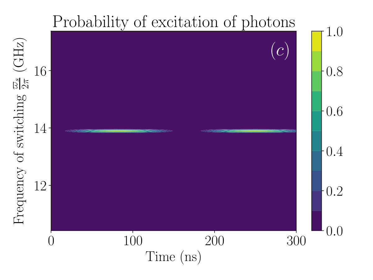 Figure 1
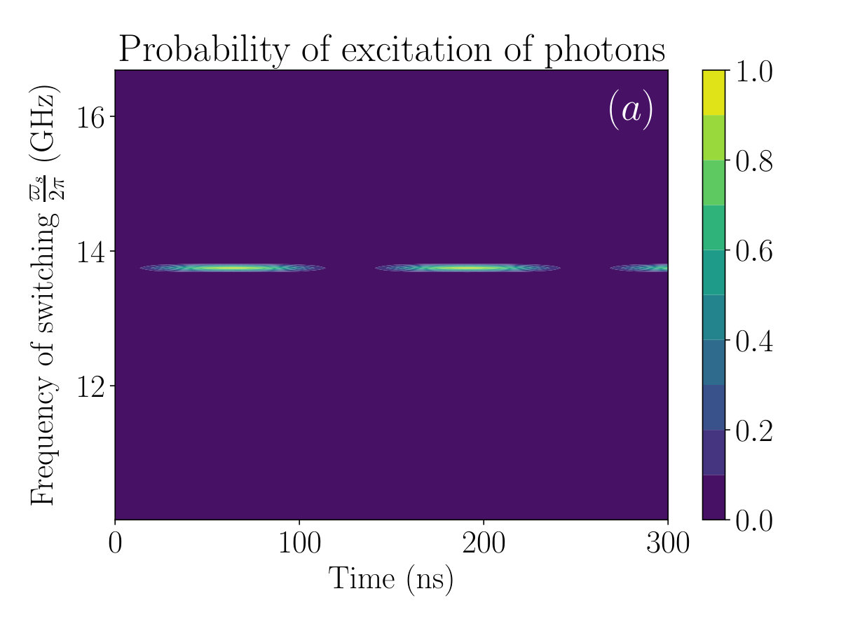 Figure 2
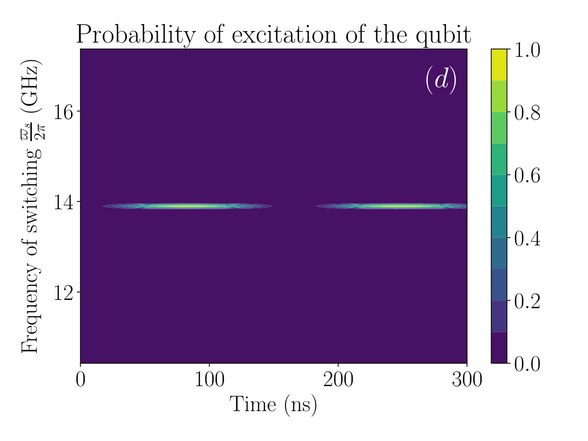 Figure 3
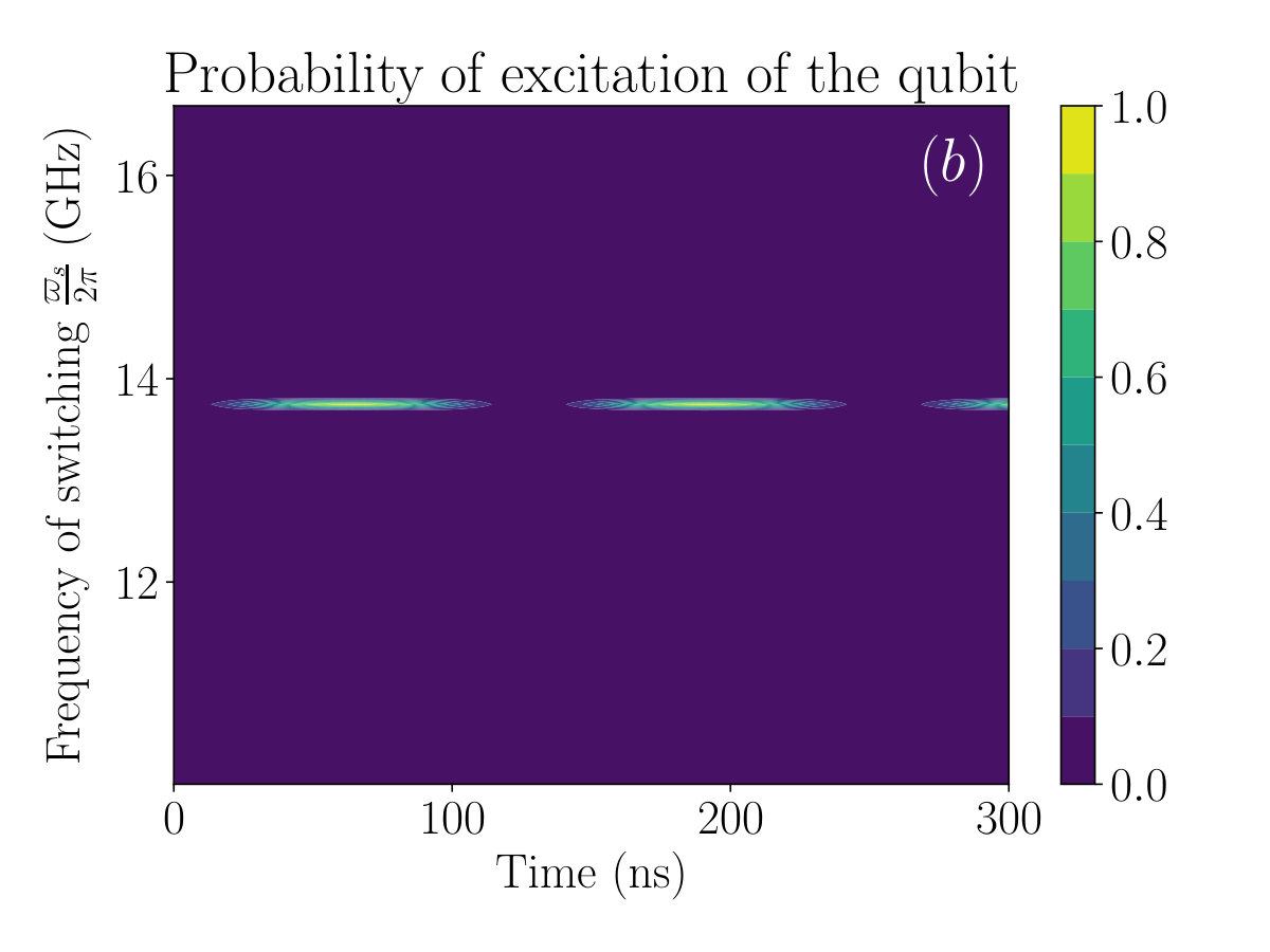 Figure 4
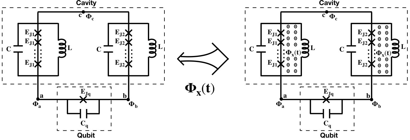 Figure 5
| Transverse coupling: | Longitudinal coupling: |
|---|---|
Peer Reviews
No public reviews on file for this paper yet. If you reviewed it on a platform where reviews are public (OpenReview, ICLR, NeurIPS, ICML), you can paste yours below so the community can read it here.
Videos
No videos yet. Explain this paper in a talk, walkthrough, or lecture? Add one.
\floatsetup
[table]capposition=top
Can the dynamical Lamb effect be observed in a superconducting circuit?
Mirko Amico1,2, Oleg L. Berman1,2 and Roman Ya. Kezerashvili1,2
1Physics Department, New York City College of Technology, The City University of New York,
Brooklyn, NY 11201, USA
2The Graduate School and University Center, The City University of New York,
New York, NY 10016, USA
Abstract
The dynamical Lamb effect is predicted to arise in superconducting circuits when the coupling of a superconducting qubit with a resonator is periodically switched ”on” and ”off” nonadiabatically. We show that by using a superconducting circuit which allows to switch between longitudinal and transverse coupling of a qubit to a resonator, it is possible of to observe the dynamical Lamb effect. The switching between longitudinal and transverse coupling can be achieved by modulating the magnetic flux through the circuit loops. By solving the Schrödinger equation for a qubit coupled to a resonator, we calculate the time evolution of the probability of excitation of the qubit and the creation of photons in the resonator due to the dynamical Lamb effect. The probability is maximum when the coupling is periodically switched between longitudinal and transverse using a square-wave or sinusoidal modulation of the magnetic flux with frequency equal to the sum of the average qubit and photon transition frequencies.
I Introduction
According to quantum field theory, the vacuum is filled with virtual particles which can be turned into real ones by specific external perturbations fulling . Phenomena of this kind are commonly referred to as quantum vacuum phenomena. Several quantum vacuum phenomena related to the peculiar nature of the quantum vacuum have been predicted casimir ; bethe , some of which have been experimentally found lamb . Other examples include the dynamical Casimir effect moore , that is the creation of real photons from the vacuum due to the fast change in boundary conditions of a cavity, and the dynamical Lamb effect dle , which is the excitation of an atom in a cavity, along with the creation of photons, due to the sudden change of its Lamb shift. To obtain an instantaneous change of the Lamb shift of the atom, the boundary conditions of the cavity must be changed nonadiabatically dle ; berman ; amico2017 ; amico2018 .
Recently, the dynamical Casimir effect has been experimentally observed in superconducting circuits wilson ; lahte . The latter provide a way to model atoms and cavities using Josephson junctions and superconducting transmission lines. The advantage of a superconducting circuit setup over real atoms and cavities lies in the possibility of tuning the parameters of the system in a short time interval, allowing us to enter the nonadiabatic regime where the mentioned quantum vacuum phenomena arise.
As noted in Ref. shapiro , the dynamical Lamb effect could be observed in a superconducting circuit as well. The nonadiabatic change in boundary conditions of the cavity needed for the dynamical Lamb effect to arise can be obtained by switching ”on” and ”off” the coupling of a qubit with a resonator. Furthermore, the periodic switching ”on” and ”off” of the qubit/resonator coupling leads to a dramatic increase in the probability of excitation of the qubit shapiro ; zhukov ; remizov ; amico2018 . In fact, the dynamical aspects of the Lamb shift in the energy levels of tunable superconducting circuits have already been investigated both theoretically gramich1 ; gramich2 and experimentally silveri . Here we focus on the case of the particular tuning required to enter the nonadiabatic regime which gives rise to the dynamical Lamb effect.
In Refs. richer2 ; richer , it was shown that it is possible to design a superconducting circuit where the qubit/resonator coupling is switched between longitudinal and transverse by modulating the magnetic flux through the circuit loops. A qubit/resonator system longitudinally coupled can be seen as a decoupled system with renormalized energy levels lang . Whereas in a qubit/resonator system with transverse coupling the qubit and the photons interact. Therefore, we suggest the possibility of observing the dynamical Lamb effect by adopting the circuit designed in Ref. richer and periodically switching between longitudinal and transverse qubit/resonator coupling. This effectively corresponds to periodically switching ”on” and ”off” of the qubit/resonator coupling, which has been shown to give rise to the dynamical Lamb effect shapiro ; zhukov ; remizov ; amico2018 .
To demonstrate the presence of the dynamical Lamb effect, we calculate the probability of excitation of the qubit and the probability of creation of photons in the resonator by solving the Schrödinger equation. The calculations show that the probabilities of excitation of the qubit and creation of photons due to the dynamical Lamb effect reach their maximum values when the coupling is periodically switched between transverse and longitudinal using a square-wave or sinusoidal modulation of the magnetic flux with frequency equal to the sum of the average qubit and photon transition frequencies.
The article is organized as follows. In Sec. II the Hamiltonian of a qubit/resonator system with longitudinal or transverse coupling is specified. In Sec. III, a superconducting circuit which allows for the switching between a longitudinally coupled Hamiltonian and a transverse one is introduced. We show how to switch between longitudinal and transverse coupling through the modulation of the magnetic flux threading the circuit. The results of numerical calculations of the time evolution of the probability of excitation of the qubit and the photons for different modulation of the magnetic flux are given in Sec. IV. The conclusions follow in Sec. V.
II Longitudinal and transverse coupling
As a first step, let us show how a system with longitudinal qubit/resonator coupling can be seen as an uncoupled system, in contrast to the case of transverse qubit/resonator coupling. The Hamiltonians of a qubit longitudinally and transversely coupled to a resonator, respectively, can be written as
[TABLE]
[TABLE]
where is the transition frequency of the qubit, is the frequency of the photons in the resonator, , and , are the creation and annihilation operators for excitations of qubit and photons, respectively, , and are the Pauli , and operators, while and are the longitudinal and transverse coupling strengths, respectively. Applying an appropriate unitary transformation lang ; billangeon , the Hamiltonian (1) can be written in a diagonal form as
[TABLE]
where is the identity operator. Since and are related by a unitary transformation, their eigenvalues are the same and they describe a qubit and a resonator with the same transition frequencies and they describe a qubit and a resonator with the same transition frequencies. Therefore, the two Hamiltonians describe systems which are characterized by the same observables. However, in (3) the qubit is now decoupled from the resonator and the zero-point energy is renormalized. In this case, the Lamb shift of the qubit is absent. On the other hand, one can not diagonalize Hamiltonian (2) by any unitary transformation, and, therefore, the qubit/resonator coupling cannot be eliminated. The latter implies that the energy levels of the qubit will be affected by the Lamb shift. So, we can regard the system with longitudinal coupling given by Eq. (1) as a system of a qubit and a resonator with the qubit/resonator coupling turned ”off” and the system with transverse coupling defined by Hamiltonian (2) as the same qubit and resonator with the qubit/resonator coupling turned ”on”. Thus, the switching between these two coupling regimes involves a change in the Lamb shift of the qubit.
III Superconducting circuit with tunable qubit/resonator coupling
Let us consider the circuit in Fig. 1 and define the branch fluxes associated with the qubit and the resonator, as and , respectively, where , and are the magnetic fluxes at the nodes , and . Following Ref. devoret , one can write the Lagrangian for the circuit in Fig. 1 by adding the contributions of each element in terms of the branch fluxes richer
[TABLE]
In Eq. (4), is the external magnetic flux threading the areas enclosed by the left and right loops, is the number of Josephson junctions in a branch of the circuit, which the same in each branch, and are the capacitance and the inductance of the loops, respectively, and are the Josephson energies of the junctions in each branch, the Josephson energy of the qubit junction and its capacitance. The Hamiltonian of the system can be found by taking the Legendre transform of the Lagrangian: , where are the indices corresponding to the qubit and resonator flux variables, respectively. This leads to the following Hamiltonian for the circuit
[TABLE]
A quantum mechanical model of the circuit can be obtained from its classical Hamiltonian by applying the standard procedure of second quantization for the qubit and resonator variables separately richer . For example, the quantum mechanical model for the resonator is obtained from Hamiltonian (5) by setting and , expanding the cosine terms up to second order in , and expressing the resonator’s variables and in terms of the operators of creation and annihilation of photons in the resonator , , respectively,
[TABLE]
which give
[TABLE]
where is the transition frequency between the energy levels of the system and is a dimensionless parameter, defined in Table 2, which accounts for the flux-dependence of the system. The Hamiltonian (7) is the Hamiltonian of a harmonic oscillator. The operators of creation and annihilation of photons in the resonator are bosonic operators which satisfy the commutation relation . With the definitions given in Eq. (6), and the commutation relation for and , one can prove that the variables and satisfy the commutation relation for conjugate variables . One can do the same for the qubit variables, starting from Hamiltonian (5), setting and , expanding the cosine terms up to second order in , and introducing the operators of creation and annihilation of resonator excitation in terms of and ,
[TABLE]
which give the following quantum mechanical Hamiltonian
[TABLE]
where is the transition frequency between the first two energy levels of the system. The operators of creation and annihilation of qubit excitation are also taken to be bosonic operators satisfying the commutation relation . Again, one can prove that the variables and satisfy the commutation relation for conjugate variables by using the commutation relation for and , together with the definitions given in Eq. (8). Since we consider only two accessible levels, we replace the the creation and annihilation operators and with and , which are used to describe excitations in a two-level system. The transition frequency between the first two levels is also adjusted to take into account the anharmonicity by replacing with . Therefore, we rewrite the Hamiltonian (9) as
[TABLE]
Hamiltonian (10) is the Hamiltonian of a quantum two-level system. To obtain a quantum mechanical Hamiltonian of the system, one can substitute the expressions for the resonator and qubit variables given in Eqs. (6) and (8), respectively, into Hamiltonian (5). In this way, one can also express the terms in Hamiltonian (5) which involve both resonator and qubit variables in the argument of the cosine, thus coupling those variables, in terms of creation and annihilation operators of the photons excited in the resonator and qubit’s excitation. Thus, getting
[TABLE]
where is the transition frequency of the resonator, is the transition frequency of the qubit and , , and are the coupling strengths. The expressions of each of the parameters in Hamiltonian (11) are given in Table 2 in the Appendix. It is important to note that all these parameters depend on time through their dependence on the external magnetic flux .
III.1 Square-wave modulation
We consider two forms of the magnetic flux modulation: a square-wave and a sinusoidal one. Let us first focus on the case of a square-wave modulation of the magnetic flux
[TABLE]
where is the Heaviside function which switches on periodically with period , where is the frequency of the switching of the magnetic flux. By switching the external magnetic flux between the values [math] and , one can tune the qubit and the resonator parameters in Hamiltonian (11) at each instant of time. This gives the instantaneous switching between transverse and longitudinal qubit/resonator coupling which can be used to give rise to the dynamical Lamb effect.
In particular, for we can write the Hamiltonian (11) as
[TABLE]
where the expression of the parameters are given in Table 1. In this case, and the Hamiltonian (13) is instantaneously equivalent to the Hamiltonian (2) of a transversely coupled qubit/resonator system, with the exception of an extra coupling term.
On the other hand, for , Hamiltonian (11) can be reduced to the following form
[TABLE]
where the expressions of are also given in Table 1. Here, , which leads to an instantaneous longitudinal qubit/resonator coupling as in (1), with a spurious coupling term. To suppress the unwanted terms and in Hamiltonian (13) and (14), respectively, we choose specific values of the parameters of the circuit.
III.2 Sinusoidal modulation
Although the square-wave modulation of the magnetic flux comes closest to the requirement of periodic and instantaneous switching ”on” and ”off” of the qubit/resonator coupling needed to observe the dynamical Lamb effect, this may be unrealistic in the experimental setting. For this reason, we turn to another type of modulation, a sinusoidal one, which can be easily obtained in experiments. In fact, a high-frequency sinusoidal magnetic flux was used in the first experimental observation of the dynamical Casimir effect wilson . This models the more realistic situation where a finite amount of time is needed to switch ”on” and ”off” the coupling of the qubit with the resonator. Thus, we take as
[TABLE]
In this case, the magnetic flux doesn’t instantaneously switch ”on” and ”off” but continuously increases or decreases to its maximum or minimum value, respectively. However, the rise time , that is the time required to increase the magnetic flux from the minimum value to the maximum value, and, vice versa, the fall time , the time needed to decrease it from the maximum value to the minimum value, are shorter than any parameter with dimension of time . Therefore, one can still consider this modulation to be nonadiabatic. The parameters of Hamiltonian (11) do not take the simple form shown in Table 1 for the case of square-wave modulation but vary continuously with the magnetic flux . These parameters can be found by substituting the sinusoidal modulation of the magnetic flux in the corresponding expressions from Table 2 in the Appendix.
IV results and discussion
We numerically solve the Schrödinger equation for the Hamiltonian (11) in the case of periodic switching between transverse and longitudinal coupling with the initial condition , where denotes the qubit in the ground state and [math] is the number of photons in the resonator. In the numerical calculations of the probabilities of excitation of the qubit and creation of photons, we use the following values of the parameters of the circuit richer :
[TABLE]
Fig. 2 shows the time dependence of the probabilities of excitation of the qubit and the photons for a range of frequencies of switching of the magnetic flux. Clearly, there is a particular value of the switching frequency which corresponds to the maximal probabilities of excitation of the qubit and the photons. Figs. 2a and 2b depict the results obtained in the case of a square-wave modulation of the magnetic flux, while the results obtained in the case of sinusoidal modulation of the magnetic flux are shown in Figs. 2c and 2d. In both cases, the value of the frequency of switching of the magnetic flux which maximize the probability of excitation of the qubit and the photons is , which is the sum of the time-averaged qubit transition frequency and the time-averaged photon transition frequency over a period of oscillation of the magnetic flux. Because of the different time-dependence of the qubit and resonator transition frequencies for the different modulations, the probability of excitation of the qubit and the photons reach their maximum value at a different frequency of switching of the magnetic flux. In the case of a square-wave modulation, the probabilities are maximum for GHz. While for the case of a sinusoidal modulation, the maximum is at GHz. Moreover, the probabilities are constant with time and close to zero for almost all other values of the frequency of switching of the magnetic flux different from .
It is crucial to note that the state , where stands for the qubit in the excited state, can only be reached from the initial state through the counter-rotating terms in Eq. (11). Since the counter-rotating terms are responsible for the presence of the Lamb shift of the qubit’s energy level, the sudden change in Lamb shift can be obtained by nonadiabatically switching these terms ”on” and ”off”. Also, when the qubit/resonator coupling is periodically switched ”on” and ”off” at a frequency equal to the sum of the qubit and the resonator average frequencies, the contribution of counter-rotating terms becomes important. This makes the dynamical Lamb effect the main channel of excitation of the qubit and the creation of photons. Thus, the transition caused by the nonadiabatic change of qubit/resonator coupling demonstrates the presence of the dynamical Lamb effect. A comparison of Figs. 2a and 2b, and Figs. 2c and 2d, clearly shows that the probabilities of excitation of the photon and the qubit coincide, indicating that the system is undergoing such transition.
V conclusion
In conclusion, we predict that the dynamical Lamb effect could arise in superconducting circuits when the coupling of a superconducting qubit with a resonator is periodically switched ”on” and ”off” nonadiabatically and demonstrate that by using a superconducting circuit which allows to switch between longitudinal and transverse coupling of a qubit to a resonator, it is possible of to observe the dynamical Lamb effect. In particular, the switching between longitudinal and transverse coupling which gives rise to the dynamical Lamb effect is achieved by turning ”on” and ”off” the magnetic flux through the loops of the superconducting circuit. If the magnetic flux is periodically turned ”on” and ”off” as a square-wave or a sinusoidal modulation with a frequency of switching equal to the sum of the average qubit and photon transition frequencies, the calculated probabilities of excitation of the qubit and the photons due to the dynamical Lamb effect reach their maximum values.
Acknowledgements.
The authors are grateful to M. Kumph, D. C. Mckay and L. Glazman for the valuable and stimulating discussions.
Appendix A
The analytical expressions of the parameters for the Hamiltonian (11) used in the calculations of the time-evolution of the probability of excitation of the qubit and photons are given in the table below richer .
The reference list from the paper itself. Each links out to its DOI / PubMed record.
- 1(1) S. A. Fulling, Aspects of quantum field theory in curved space-time (Cambridge Univ. Press, Cambridge, 1989).
- 2(2) H. B. G. Casimir, Proc. K. Ned. Akad. Wet. B 51 , 793 (1948).
- 3(3) H. A. Bethe, Phys. Rev. 72 , 339 (1947).
- 4(4) W. E. Lamb, Jr. and R. C. Retherford, Phys. Rev. 72 , 241 (1947).
- 5(5) G. Moore, J. Math. Phys. 11 , 2679 (1970).
- 6(6) N. B. Narozhny, A. M. Fedotov, and Yu. E. Lozovik, Phys. Rev. A 64 , 053807 (2001).
- 7(7) O. L. Berman, R. Ya. Kezerashvili, and Yu. E. Lozovik, Phys. Rev. A 94 , 052308 (2016).
- 8(8) M. Amico, O. L. Berman, and R. Ya. Kezerashvili, Phys. Rev. A 96 , 032328 (2017).