SOFIA {\it FORCAST} Photometry of 12 Extended Green Objects in the Milky Way
Allison P. M. Towner, Crystal L. Brogan, Todd R. Hunter, Claudia J., Cyganowski, Rachel K. Friesen

TL;DR
This study uses SOFIA FORCAST photometry to analyze 12 extended green objects in the Milky Way, constructing their spectral energy distributions to understand their evolutionary stage and physical properties.
Contribution
First mid-infrared imaging and photometry of 12 EGOs with SOFIA, combined with multi-wavelength data and modeling to characterize their physical parameters and evolutionary status.
Findings
Median luminosity-to-mass ratio suggests a transitional evolutionary stage.
Models indicate typical protostar radius around 10 solar radii.
Objects are likely in a cooler, younger phase of IR-bright stage.
Abstract
Massive young stellar objects are known to undergo an evolutionary phase in which high mass accretion rates drive strong outflows. A class of objects believed to trace this phase accurately is the GLIMPSE Extended Green Object (EGO) sample, so named for the presence of extended 4.5 m emission on sizescales of 0.1 pc in \textit{Spitzer} images. We have been conducting a multi-wavelength examination of a sample of 12 EGOs with distances of 1 to 5 kpc. In this paper, we present mid-infrared images and photometry of these EGOs obtained with the SOFIA telescope, and subsequently construct SEDs for these sources from the near-IR to sub-millimeter regimes using additional archival data. We compare the results from greybody models and several publicly-available software packages which produce model SEDs in the context of a single massive protostar. The models yield typical…
Click any figure to enlarge with its caption.
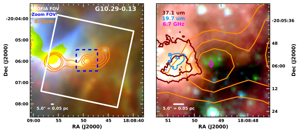 Figure 1
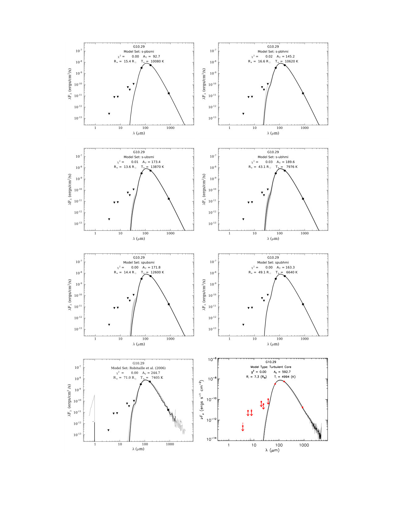 Figure 2
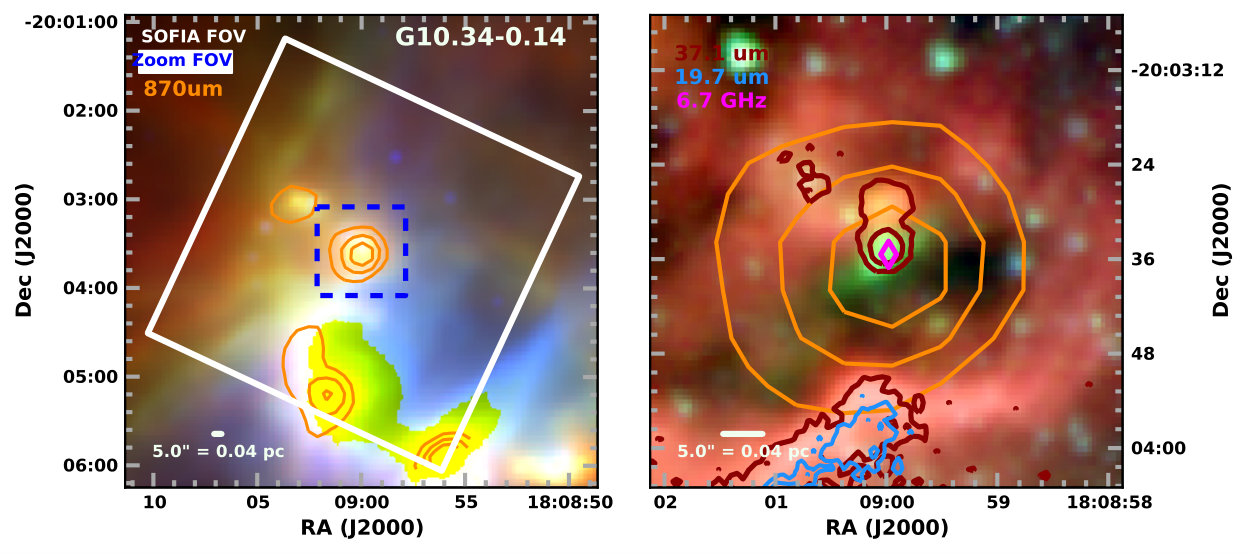 Figure 3
 Figure 4
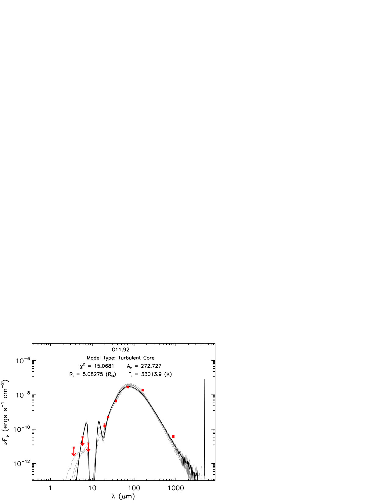 Figure 5
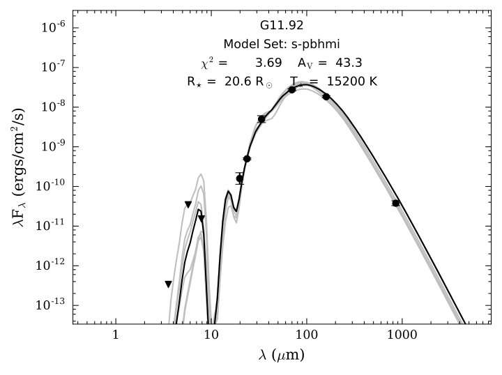 Figure 6
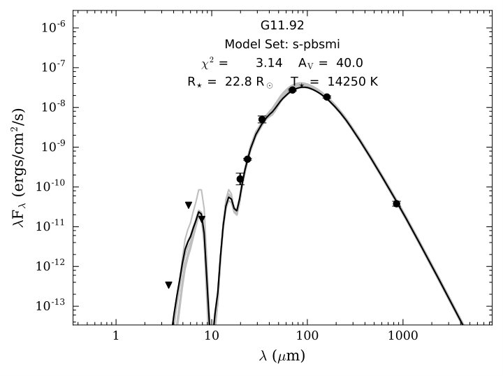 Figure 7
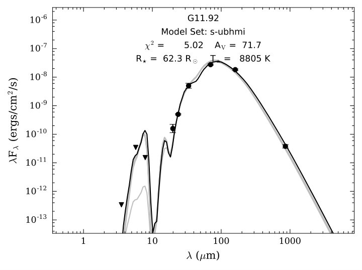 Figure 8
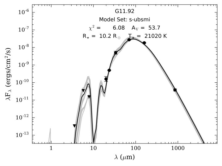 Figure 9
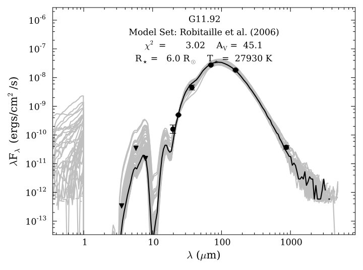 Figure 10
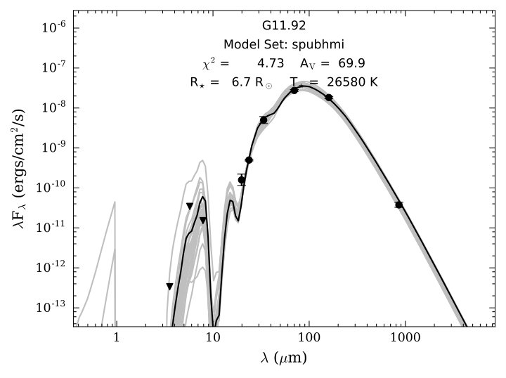 Figure 11
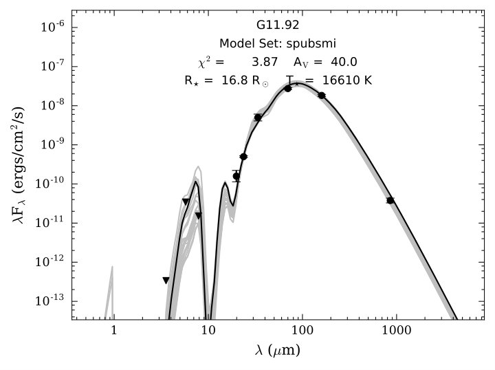 Figure 12
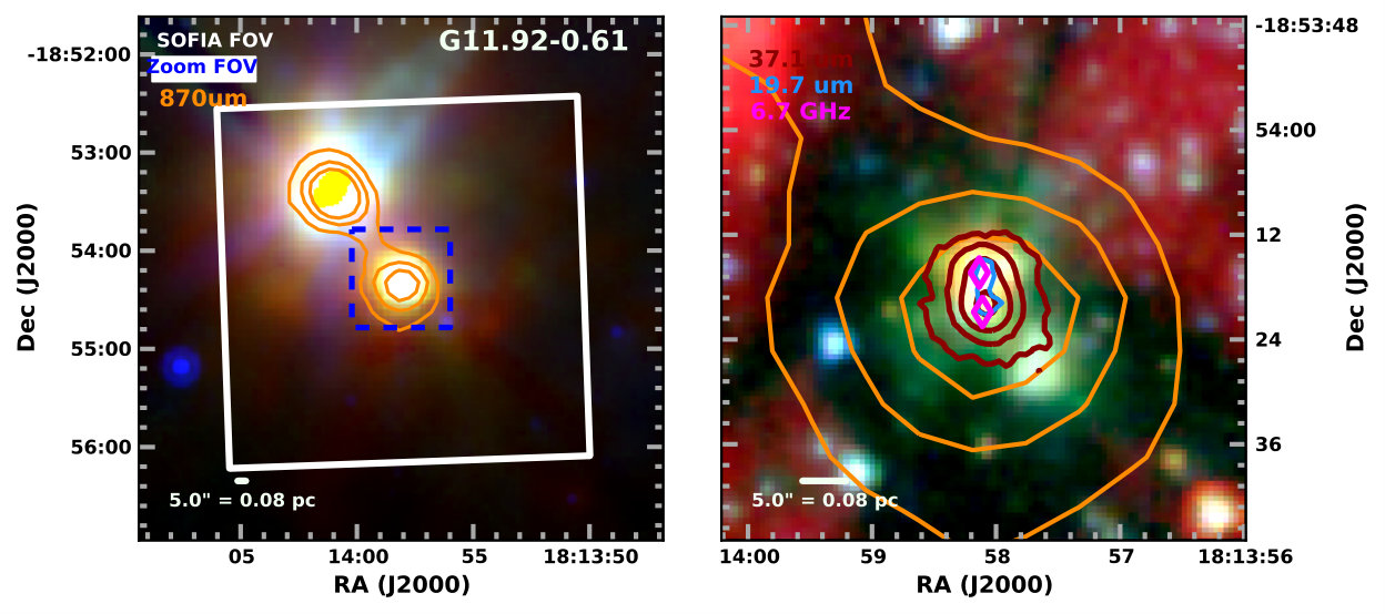 Figure 13
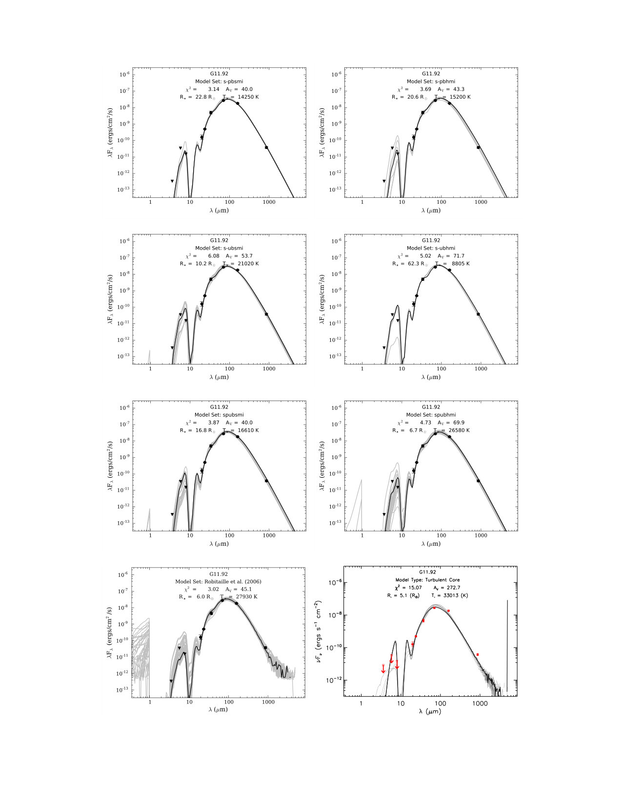 Figure 14
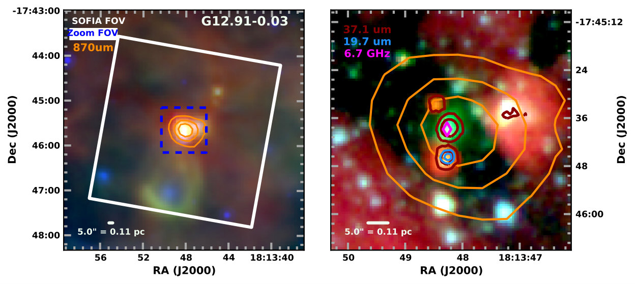 Figure 15
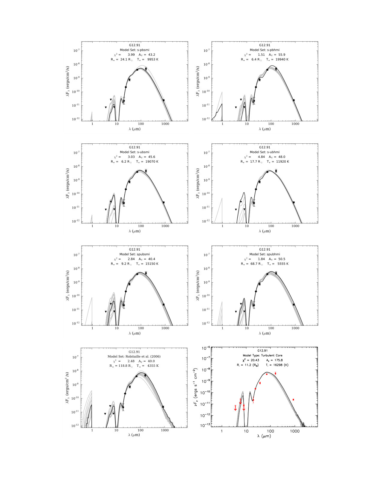 Figure 16
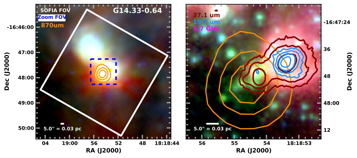 Figure 17
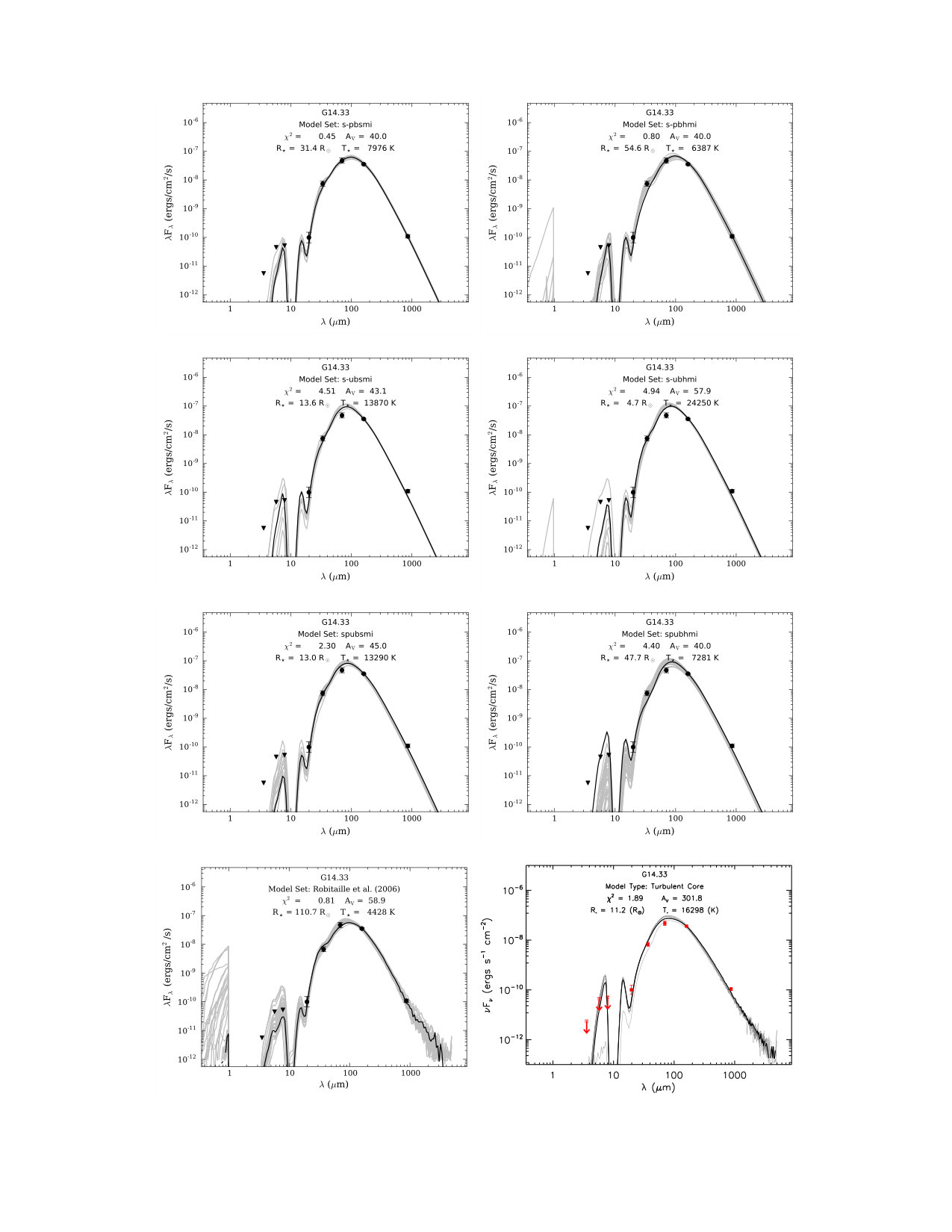 Figure 18
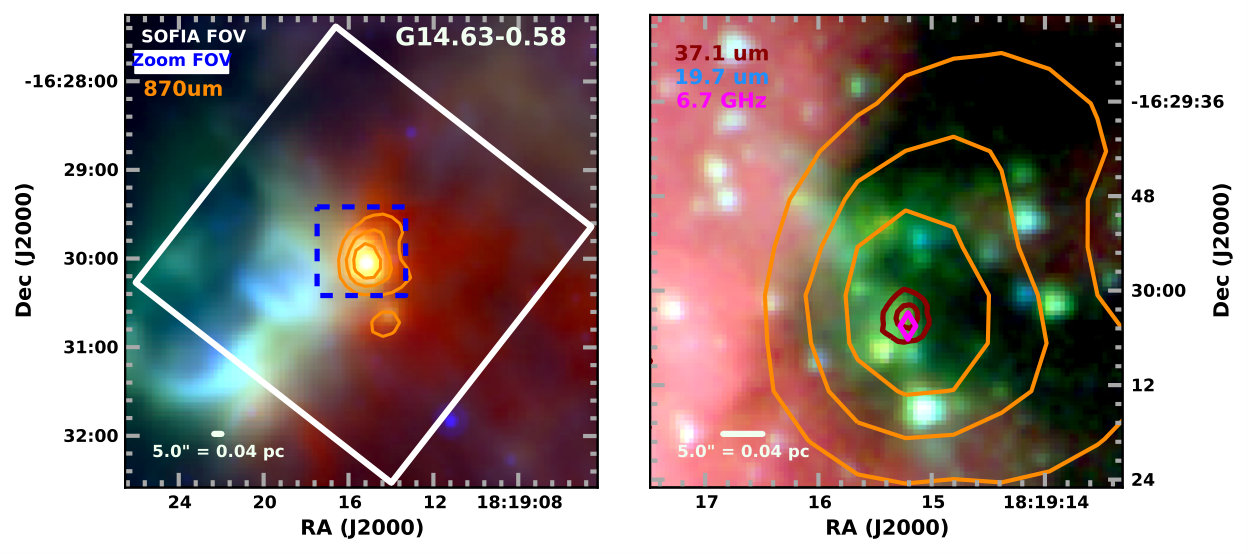 Figure 19
 Figure 20
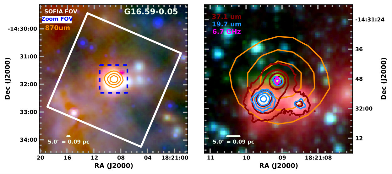 Figure 21
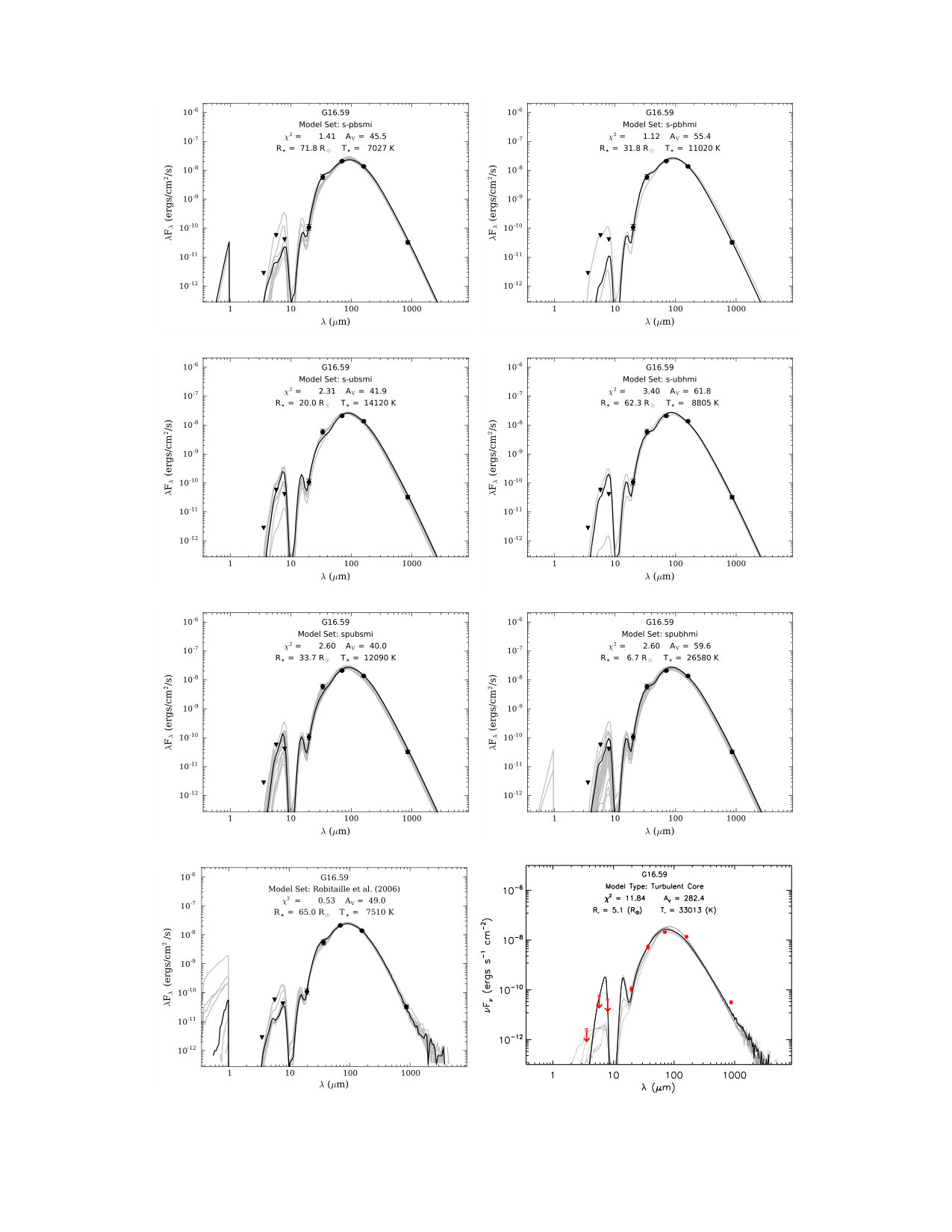 Figure 22
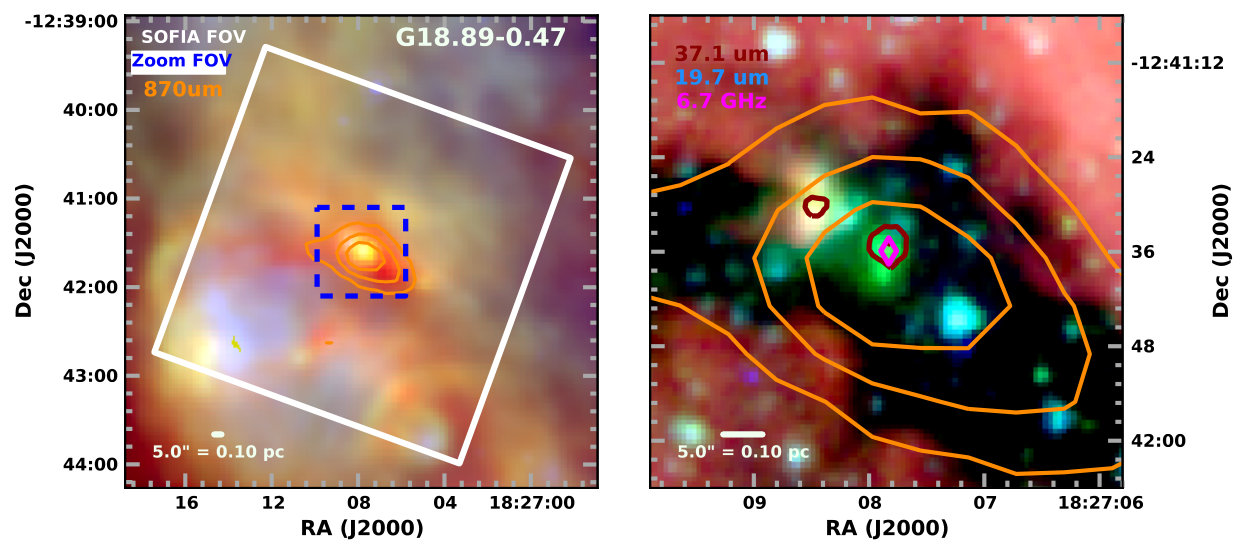 Figure 23
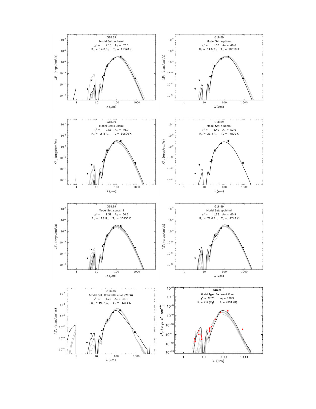 Figure 24
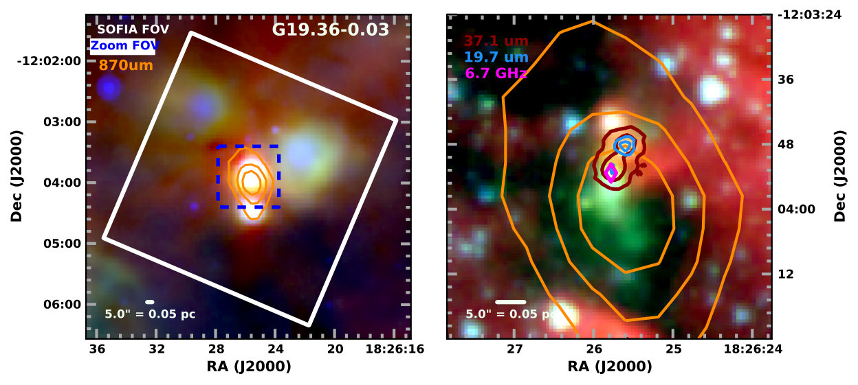 Figure 25
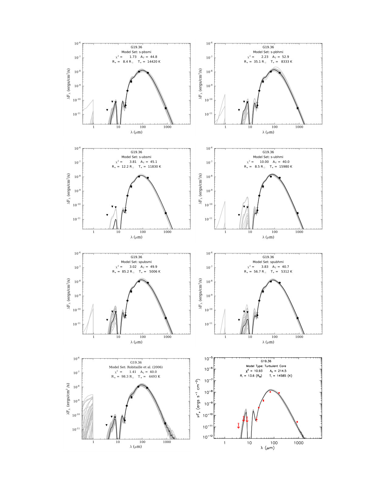 Figure 26
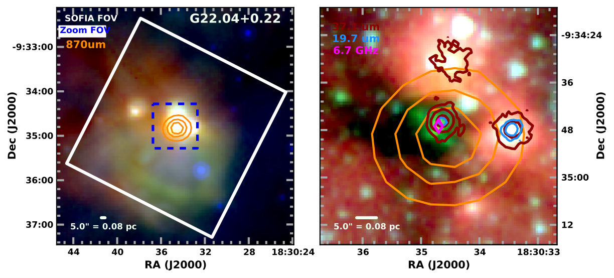 Figure 27
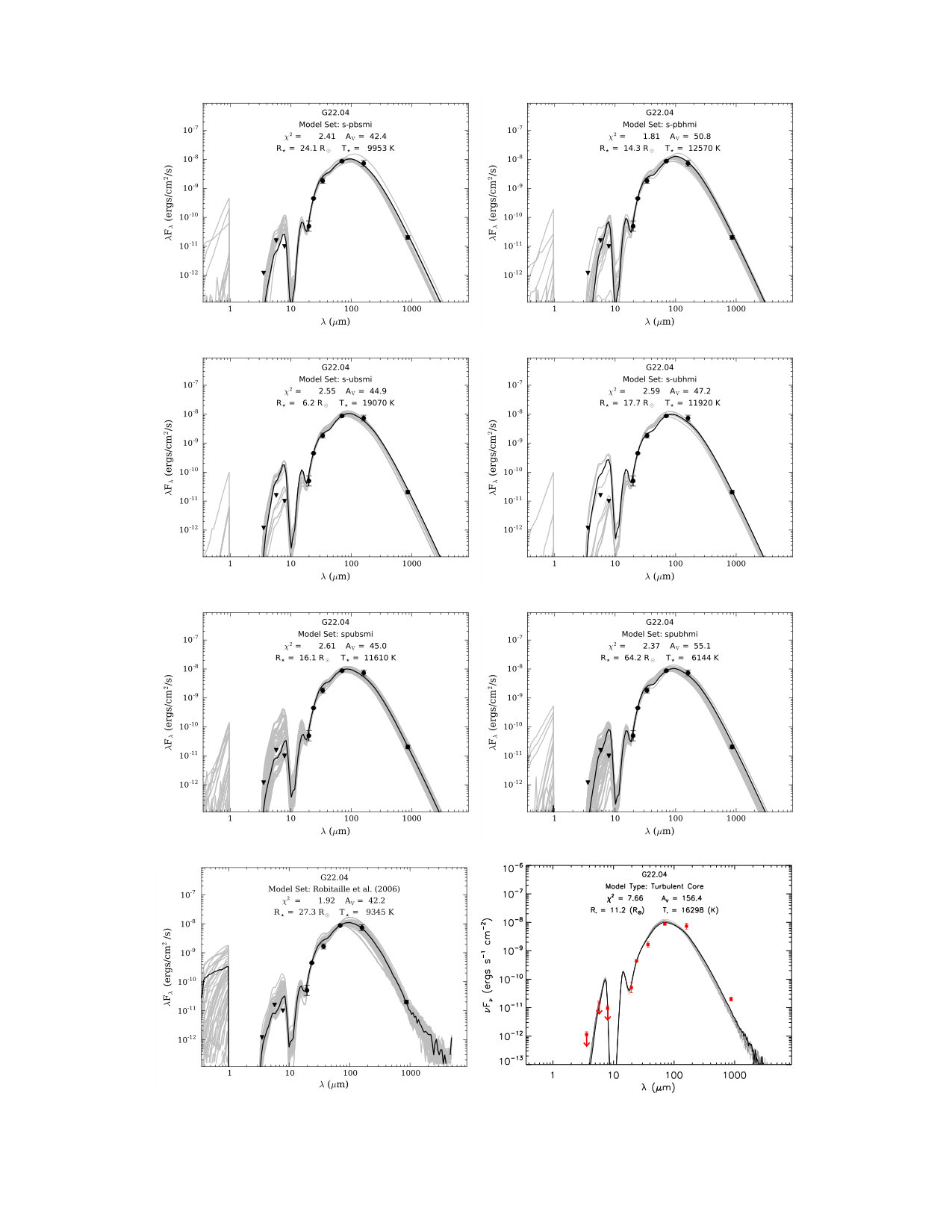 Figure 28
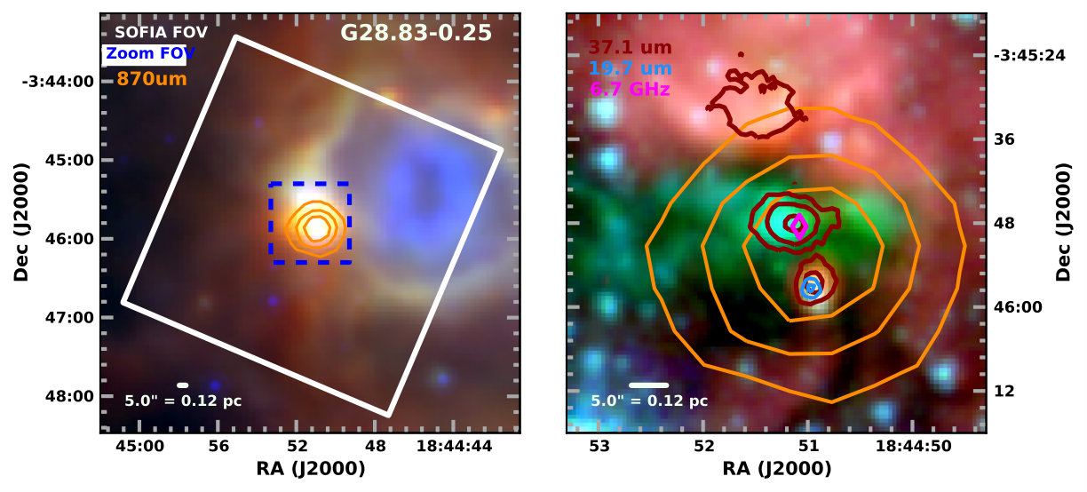 Figure 29
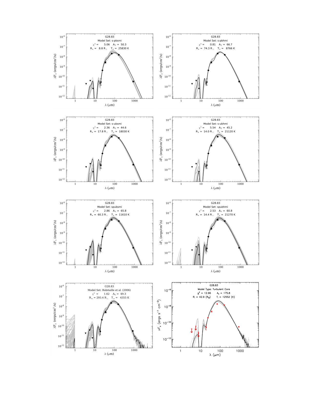 Figure 30
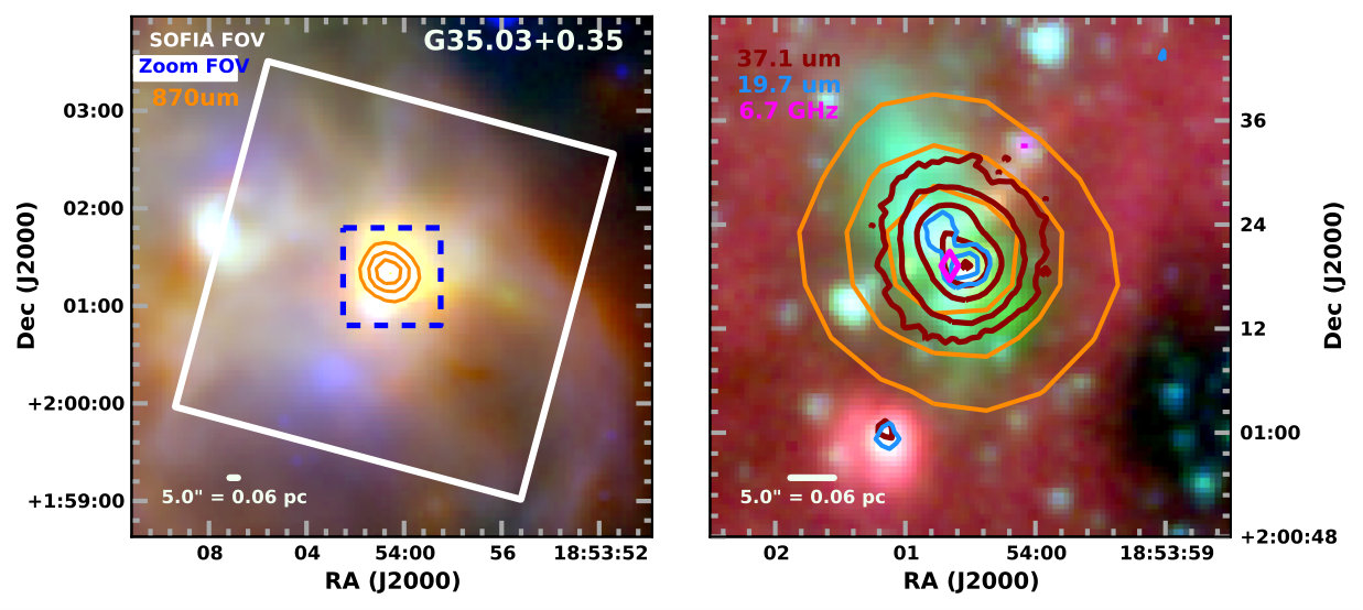 Figure 31
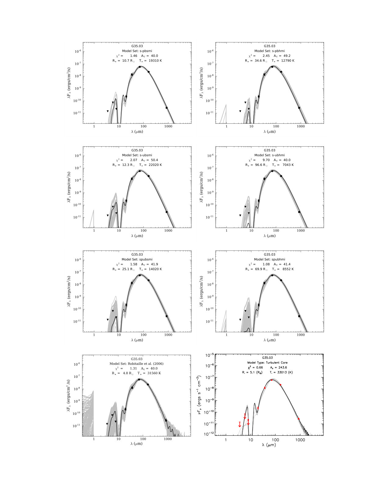 Figure 32
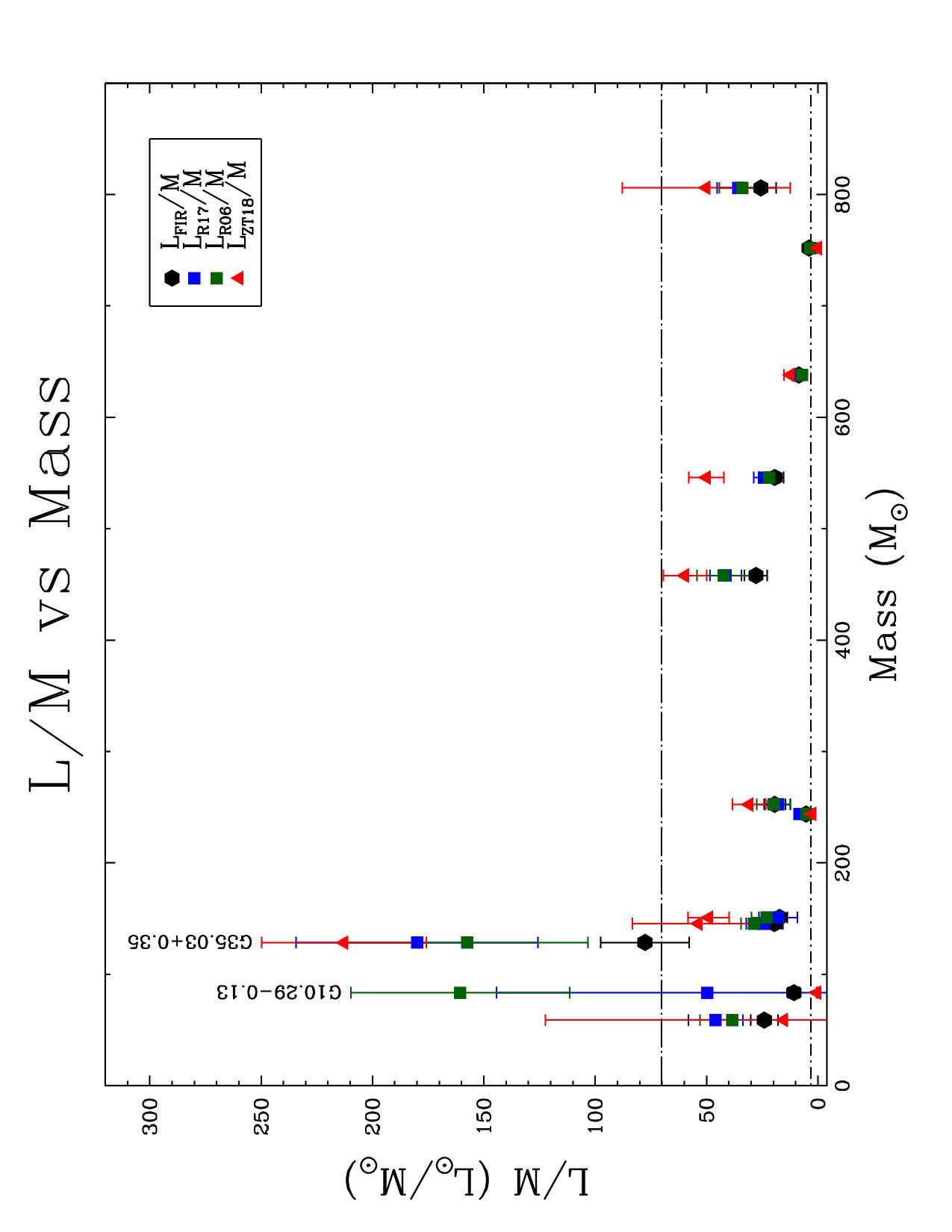 Figure 33
| Source | Distanceb | EGOc | IRDCd | H2Oe | CH3OH Masers (GHz)f | |||
|---|---|---|---|---|---|---|---|---|
| (km s-1) | (kpc) | Cat | Maser | 6.7g | 44h | 95i | ||
| G10.290.13 | 14 | 1.9 | 2 | Y | Y | Y | Y | Y |
| G10.340.14 | 12 | 1.6 | 2 | Y | Y | Y | Y | Y |
| G11.920.61 | 36 | 3.38 (3.5) | 1 | Y | Y | Y | Y | Y |
| G12.910.03 | 57 | 4.5 | 1 | Y | Y | Y | ? | Y |
| G14.330.64 | 23 | 1.13 (2.3) | 1 | Y | Y | ? | Y | Y |
| G14.630.58 | 19 | 1.83 (1.9) | 1 | Y | Y | Y | ? | Y |
| G16.590.05 | 60 | 3.58 (4.2) | 2 | N | Y | Y | ? | Y |
| G18.890.47 | 66 | 4.2 | 1 | Y | Y | Y | Y | Y |
| G19.360.03 | 27 | 2.2 | 2 | Y | N | Y | Y | Y |
| G22.040.22 | 51 | 3.4 | 1 | Y | Y | Y | Y | Y |
| G28.830.25 | 87 | 4.8 | 1 | Y | Y | Y | Y | ? |
| G35.030.35 | 53 | 2.32 (3.2) | 1 | Y | Y | Y | Y | Y |
| Source | Pointing Center (J2000) | Obs. Datea | TOSb | (MAD)c | ||
|---|---|---|---|---|---|---|
| RA | Dec | (s) | 37 m | 19 m | ||
| G10.290.13 | 18:08:49.2 | -20:05:59.3 | 2016 July 13 | 502 | 0.26 | 0.08 |
| G10.340.14 | 18:08:59.9 | -20:03:37.3 | 2016 Sept 27 | 626 | 0.30 | 0.07 |
| G11.920.61 | 18:13:58.0 | -18:54:19.3 | 2016 July 12 | 604 | 0.22 | 0.07 |
| G12.910.03 | 18:13:48.1 | -17:45:41.3 | 2016 July 19 | 1000 | 0.18 | 0.04 |
| G14.330.64 | 18:18:54.3 | -16:47:48.3 | 2016 July 12 | 593 | 0.24 | 0.07 |
| G14.630.58 | 18:19:15.3 | -16:29:57.3 | 2016 July 13 | 641 | 0.22 | 0.07 |
| G16.590.05 | 18:21:09.0 | -14:31:50.3 | 2016 July 20 | 810 | 0.19 | 0.04 |
| G18.890.47 | 18:27:07.8 | -12:41:38.3 | 2016 Sept 27 | 626 | 0.25 | 0.06 |
| G19.360.03 | 18:26:25.7 | -12:03:56.3 | 2016 Sept 20 | 285 | 0.46 | 0.09 |
| G22.040.22 | 18:30:34.6 | -09:34:49.3 | 2016 Sept 20 | 642 | 0.21 | 0.05 |
| G28.830.25 | 18:44:51.2 | -03:45:50.3 | 2016 Sept 27 | 470 | 0.26 | 0.07 |
| G35.030.35 | 18:54:00.4 | +02:01:15.7 | 2016 Sept 22 | 500 | 0.29 | 0.08 |
| EGO | Sourcea | Coordinates (J2000)b | Fitted Sizeb | 19 m Fluxc | 37 m Fluxc | ||
|---|---|---|---|---|---|---|---|
| RA (h m s) | Dec (∘ ) | Major Minor () | PA (∘) | Density (Jy) | Density (Jy) | ||
| G10.290.13 | a | ¡0.40 | ¡1.3 | ||||
| G10.340.14 | a | 18:09:00.001 (0.003) | -20:03:34.53 (0.04) | 1.41 1.01 (0.31 0.45) | 97 (31) | ¡0.36 | 14 (3) |
| b | 18:09:00.02 (0.02) | -20:03:28.8 (0.2) | 4.55 2.97 (0.71 0.61) | 97 (15) | 0.7 (0.2) | 9 (2) | |
| G11.920.61 | a | 18:13:58.078 (0.002) | -18:54:20.16 (0.04) | 2.63 2.39 (0.1 0.05) | 32 (9) | 1.1 (0.4) | 57 (12) |
| b | 18:13:58.113 (0.008) | -18:54:16.25 (0.09) | 3.41 2.59 (0.14 0.13) | 100 (6) | 0.7 (0.3) | 25 (5) | |
| G12.910.03 | a | 18:13:48.227 (0.004) | -17:45:38.46 (0.06) | 2.17 1.58 (0.26 0.30) | 148 (17) | 0.2 (0.1) | 9 (2) |
| b | 18:13:48.276 (0.005) | -17:45:45.91 (0.09) | 2.01 1.49 (0.40 0.48) | 160 (29) | 0.7 (0.2) | 6 (1) | |
| c | 18:13:48.44 (0.01) | -17:45:32.5 (0.2) | 1.43 1.11 (0.84 0.91) | 35 (140) | ¡0.20 | 2.2 (0.6) | |
| G14.330.64 | a | 18:18:54.232 (0.003) | -16:47:48.40 (0.06) | 5.40 3.41 (0.08 0.06) | 4.2 (1.3) | 0.7 (0.3) | 85 (17) |
| b | 18:18:53.36 (0.01) | -16:47:42.3 (0.1) | 11.42 10.23 (0.15 0.13) | 107 (5) | 22 (5) | 200 (41) | |
| c | 18:18:54.64 (0.01) | -16:47:49.6 (0.1) | point source | pt. src. | ¡0.33 | 7 (1) | |
| G14.630.58 | a | 18:19:15.225 (0.009) | -16:30:03.3 (0.1) | 3.60 2.91 (0.41 0.39) | 59 (22) | ¡0.34 | 10 (2) |
| G16.590.05 | a | 18:21:09.124 (0.002) | -14:31:48.79 (0.03) | 2.47 2.41 (0.04 0.04) | 89 (29) | 0.7 (0.2) | 67 (14) |
| b | 18:21:09.509 (0.001) | -14:31:55.88 (0.01) | 6.14 5.18 (0.1 0.09) | 141 (4) | 5 (1) | 68 (14) | |
| c | 18:21:08.511 (0.001) | -14:31:57.92 (0.01) | 1.91 1.91 (0.1 0.1) | 167 (360) | 0.8 (0.3) | 6 (1) | |
| G18.890.47 | a | 18:27:07.835 (0.008) | -12:41:35.1 (0.1) | 1.93 1.85 (0.70 0.72) | 167 (307) | ¡0.31 | 5 (1) |
| b | 18:27:08.46 (0.03) | -12:41:29.8 (0.5) | 5.0 3.3 (1.7 1.5) | 23 (31) | ¡0.31 | 4 (1) | |
| G19.360.03 | a | 18:26:25.750 (0.005) | -12:03:52.57 (0.07) | 2.69 2.48 (0.28 0.28) | 70 (52) | 0.3 (0.1) | 24 (5) |
| b | 18:26:25.591 (0.009) | -12:03:47.9 (0.1) | 3.78 2.56 (0.41 0.39) | 84 (12) | 1.7 (0.5) | 20 (4) | |
| G22.040.22 | a | 18:30:34.635 (0.003) | -09:34:45.74 (0.04) | 2.13 1.57 (0.13 0.15) | 135 (9) | 0.4 (0.2) | 21 (4) |
| b | 18:30:33.43 (0.01) | -09:34:47.9 (0.2) | 4.81 4.34 (0.40 0.38) | 95 (32) | 1.8 (0.4) | 14 (3) | |
| G28.830.25 | a | 18:44:51.138 (0.001) | -03:45:48.05 (0.01) | 4.41 2.53 (0.16 0.14) | 87.5 (0.1) | 0.3 (0.2) | 32 (7) |
| b | 18:44:50.938 (0.008) | -03:45:56.5 (0.2) | 2.61 1.34 (0.42 0.63) | 159 (12) | 1.1 (0.3) | 8 (2) | |
| G35.030.35 | a | 18:54:00.524 (0.003) | +02:01:19.16 (0.04) | 3.64 3.10 (0.03 0.03) | 115 (2) | 1.5 (0.4) | 160 (31) |
| b | 18:54:00.700 (0.007) | +02:01:23.2 (0.1) | 5.47 3.91 (0.09 0.07) | 131 (2) | 0.8 (0.3) | ||
| EGO | Source | Aperturea | Annulusa | Aperture Correctionb | Aperture-Corrected Flux Density (mJy) | ||||
|---|---|---|---|---|---|---|---|---|---|
| Radius () | Radii () | 3.6 m | 5.8 m | 8.0 m | 3.6 m | 5.8 m | 8.0 m | ||
| G10.290.13 | a | 3.6 | 3.6 to 8.4 | 1.125 | 1.135 | 1.221 | 0.4 (0.3) | 15 (3) | 22 (8) |
| G10.340.14 | a | 3.6 | 3.6 to 8.4 | 1.125 | 1.135 | 1.221 | 16.0 (0.8) | 94 (6) | 99 (14) |
| b | 3.6 | 3.6 to 8.4 | 1.125 | 1.135 | 1.221 | 11.2 (0.6) | 137 (7) | 350 (21) | |
| G11.920.61 | a | 2.4 | 2.4 to 7.2 | 1.215 | 1.366 | 1.568 | 10.0 (0.4) | 66 (3) | 40 (2) |
| b | 2.4 | 2.4 to 7.2 | 1.215 | 1.366 | 1.568 | 22.9 (0.9) | 193 (7) | 152 (6) | |
| G12.910.03 | a | 3.6 | 3.6 to 8.4 | 1.125 | 1.135 | 1.221 | 8.7 (0.4) | 52 (3) | 20 (5) |
| b | 4.8 | 14.4 to 24.0 | 1.070 | 1.076 | 1.087 | 1.3 (0.2) | 55 (4) | 130 (13) | |
| c | 3.6 | 3.6 to 8.4 | 1.125 | 1.135 | 1.221 | 0.5 (0.2) | 15 (2) | 34 (5) | |
| G14.330.64 | a | 4.8 | 14.4 to 24.0 | 1.070 | 1.076 | 1.087 | 6.6 (0.4) | 86 (4) | 136 (9) |
| b | 12.0 | 14.4 to 24.0 | 1.000 | 1.000 | 1.000 | 141 (6) | 1600 (70) | 4300 (180) | |
| c | 3.6 | 3.6 to 8.4 | 1.125 | 1.135 | 1.221 | 2.1 (0.2) | 26 (1) | 31 (3) | |
| G14.630.58 | a | 2.4 | 2.4 to 7.2 | 1.215 | 1.366 | 1.568 | 0.9 (0.1) | 10.5 (0.1) | 13 (2) |
| G16.590.05 | a | 3.6 | 3.6 to 8.4 | 1.125 | 1.135 | 1.221 | 3.3 (0.3) | 108 (5) | 107 (7) |
| b | 6.0 | 6.0 to 12.0 | 1.060 | 1.063 | 1.084 | 60 (3) | 740 (30) | 1840 (80) | |
| c | 6.0 | 6.0 to 12.0 | 1.060 | 1.063 | 1.084 | 43 (2) | 330 (15) | 820 (40) | |
| G18.890.47 | a | 4.8 | 14.4 to 24.0 | 1.070 | 1.076 | 1.087 | 4.6 (0.6) | 46.2 (0.4) | 20 (11) |
| b | 4.8 | 14.4 to 24.0 | 1.070 | 1.076 | 1.087 | 22 (1) | 104 (6) | 200 (15) | |
| G19.360.03 | a | 4.8 | 14.4 to 24.0 | 1.070 | 1.076 | 1.087 | 24 (1) | 151 (7) | 190 (12) |
| b | 3.6 | 3.6 to 8.4 | 1.125 | 1.135 | 1.221 | 11.0 (0.5) | 101 (4) | 220 (10) | |
| G22.040.22 | a | 4.8 | 14.4 to 24.0 | 1.070 | 1.076 | 1.087 | 1.4 (0.3) | 30 (2) | 26 (6) |
| b | 9.6 | 14.4 to 24.0 | 1.011 | 1.011 | 1.017 | 79 (4) | 791 (32) | 1980 (83) | |
| G28.830.25 | a | 4.8 | 14.4 to 24.0 | 1.070 | 1.076 | 1.087 | 23 (1) | 77 (5) | 17 (8) |
| b | 4.8 | 14.4 to 24.0 | 1.070 | 1.076 | 1.087 | 8.0 (0.6) | 91 (5) | 220 (13) | |
| G35.030.35 | a | 3.6 | 3.6 to 8.4 | 1.125 | 1.135 | 1.221 | 17.0 (0.8) | 140 (6) | 58 (6) |
| b | 3.6 | 3.6 to 8.4 | 1.125 | 1.135 | 1.221 | 30 (1) | 121 (6) | 34 (6) | |
| Stara | Coordinates (J2000)b | Catalog Flux | Fitted Flux | Flux Ratio | |
|---|---|---|---|---|---|
| RA (h m s) | Dec (∘ ) | (mJy) | (mJy) | ||
| 1 | 18:30:32.40 | -09:35:47.25 | 1950 (39) | 1220 (40) | 1.60 |
| 2 | 18:30:12.78 | -09:36:47.99 | 1980 (36) | 1250 (38) | 1.58 |
| 3 | 18:30:53.95 | -09:39:51.27 | 2960 (55) | 1870 (71) | 1.58 |
| 4 | 18:30:46.32 | -09:32:28.89 | 1230 (23) | 770 (23) | 1.60 |
| 5 | 18:30:48.45 | -09:36:00.11 | 780 (14) | 490 (17) | 1.59 |
| EGO | Source | Coordinates (J2000)a | Fitted Fluxb | Aperture-Correctedc | |
|---|---|---|---|---|---|
| RA (h m s) | Dec (∘ ) | Density (Jy) | Fitted Flux (Jy) | ||
| G10.290.13 | a | ¡0.28 | |||
| G10.340.14 | a | 18:08:59.989 (0.004) | -20:03:34.97 (0.06) | 0.77 (0.03) | 1.23 (0.08) |
| b | 18:09:00.017 (0.003) | -20:03:28.75 (0.05) | 1.51 (0.04) | 2.4 (0.1) | |
| G11.920.61 | a | 18:13:58.065 (0.001) | -18:54:21.26 (0.01) | 2.484 (0.003) | 4.0 (0.2) |
| b | 18:13:58.122 (0.001) | -18:54:14.97 (0.01) | 2.262 (0.003) | 3.6 (0.2) | |
| G12.910.03 | a | 18:13:48.233 (0.002) | -17:45:38.19 (0.03) | 1.11 (0.02) | 1.77 (0.09) |
| b | 18:13:48.283 (0.001) | -17:45:46.21 (0.01) | 1.50 (0.01) | 2.4 (0.1) | |
| c | 18:13:48.469 (0.004) | -17:45:31.77 (0.04) | 0.28 (0.01) | 0.45 (0.03) | |
| G14.330.64 | a | confused | |||
| b | saturated | ||||
| c | confused | ||||
| G14.630.58 | a | 18:19:15.221 (0.001) | -16:30:03.26 (0.02) | 0.683 (0.009) | 1.09 (0.06) |
| G16.590.05 | a | saturated | |||
| b | saturated | ||||
| c | confused | ||||
| G18.890.47 | a | 18:27:07.82 (0.01) | -12:41:35.1 (0.2) | 0.34 (0.04) | 0.54 (0.07) |
| b | 18:27:08.45 (0.01) | -12:41:29.5 (0.2) | 0.64 (0.07) | 1.0 (0.1) | |
| G19.360.03 | a | 18:26:25.782 (0.001) | -12:03:53.73 (0.01) | 2.356 (0.005) | 3.8 (0.2) |
| b | 18:26:25.569 (0.001) | -12:03:48.13 (0.01) | 3.371 (0.006) | 5.4 (0.3) | |
| G22.040.22 | a | 18:30:34.627 (0.001) | -09:34:46.24 (0.02) | 2.23 (0.02) | 3.6 (0.2) |
| b | 18:30:33.432 (0.001) | -09:34:48.39 (0.01) | 2.79 (0.02) | 4.4 (0.2) | |
| G28.830.25 | a | 18:44:51.136 (0.001) | -03:45:47.845 (0.009) | 2.230 (0.008) | 3.6 (0.2) |
| b | 18:44:50.931 (0.001) | -03:45:56.506 (0.009) | 2.362 (0.008) | 3.8 (0.2) | |
| G35.030.35 | a | saturated | |||
| b | saturated | ||||
| EGO | Source | Hi-GALa | 70 m Fluxb | 160 m Fluxb | 870 m Flux |
|---|---|---|---|---|---|
| 70 m Notes | (Jy) | (Jy) | (Jy) | ||
| G10.290.13 | a | 75 (6) | 298 (30) | 5.0 (0.8) | |
| G10.340.14 | a | 280 (20) | 590 (49) | 6 (1) | |
| b | assuming all emission from a | ||||
| G11.920.61 | a | 640 (33) | 980 (58) | 11 (2) | |
| b | assuming all emission from a | ||||
| G12.910.03 | a | 96 (6) | 270 (52) | 7 (1) | |
| b | assuming all emission from a | ||||
| c | assuming all emission from a | ||||
| G14.330.64 | a | 1130 (190) | 1940 (120) | 32 (4) | |
| b | assuming all emission from a | ||||
| c | assuming all emission from a | ||||
| G14.630.58 | a | 130 (8) | 390 (30) | 15 (2) | |
| G16.590.05 | a | 490 (26) | 740 (48) | 9 (1) | |
| b | assuming all emission from a | ||||
| c | assuming all emission from a | ||||
| G18.890.47 | a | sources a and b fit with imfit | 48 (2) | 180 (27) | 10 (2) |
| b | sources a and b fit with imfit | 19.6 (0.2) | |||
| G19.360.03 | a | 250 (14) | 470 (41) | 8 (1) | |
| b | assuming all emission from a | ||||
| G22.040.22 | a | sources a and b fit with imfit | 204 (10) | 400 (94) | 5.9 (0.8) |
| b | sources a and b fit with imfit | 59 (3) | |||
| G28.830.25 | a | 510 (65) | 870 (60) | 10 (1) | |
| b | assuming all emission from a | ||||
| G35.030.35 | a | 1350 (71) | 1230 (84) | 8 (1) | |
| b | assuming all emission from a |
| EGO | Distancea | Temperatures (K) | Masses (M⊙) | L | ||
|---|---|---|---|---|---|---|
| (kpc) | T | T | Greybody | NH3-derivedd | (103 ) | |
| G10.290.13 | 1.9 | 24 (1) | 21.19 (0.17) | 76 | 91 | 0.90 |
| G10.340.14 | 1.6 | 26 (1) | 28.23 (0.38) | 62 | 56 | 1.42 |
| G11.920.61 | 3.38 (3.5) | 27 (1) | 26.27 (0.19) | 450 | 466 | 12.76 |
| G12.910.03 | 4.5 | 23 (1) | 23.56 (0.31) | 649 | 627 | 5.49 |
| G14.330.64 | 1.13 (2.3) | 29 (2) | 25.26 (0.17) | 132 | 159 | 2.84 |
| G14.630.58 | 1.83 (1.9) | 22 (1) | 20.76 (0.32) | 234 | 254 | 1.31 |
| G16.590.05 | 3.58 (4.2) | 26 (1) | 20.51 (0.38) | 456 | 636 | 10.57 |
| G18.890.47 | 4.2 | 22 (1) | 28.24 (0.19) | 879 | 625 | 3.04 |
| G19.360.03 | 2.2 | 26 (1) | 24.90 (0.31) | 147 | 155 | 2.61 |
| G22.040.22 | 3.4 | 26 (1) | 26.71 (0.49) | 257 | 248 | 4.90 |
| G28.830.25 | 4.8 | 26 (1) | 28.27 (0.50) | 851 | 761 | 20.62 |
| G35.030.35 | 2.32 (3.2) | 33 (1) | 29.54 (0.92) | 119 | 138 | 9.98 |
| Source | Robitaille (2017)a,b | Robitaille et al. (2006)a | Zhang & Tan (2018)a | ||||||||||
|---|---|---|---|---|---|---|---|---|---|---|---|---|---|
| Name | Model | () | (K) | (103 ) | () | (K) | (103 ) | () | (K) | (103 ) | |||
| G10.290.13 | spubhmi | 49.1 | 6640 | 4.15 | 0.0003 | 71.0 | 7405 | 13.41 | 0.002 | 7.3 | 4994 | 0.03 | 0.001 |
| G10.340.14 | s-pbhmi | 27.5 | 7980 | 2.71 | 1.51 | 79.3 | 4492 | 2.27 | 1.45 | 21.7 | 6835 | 0.91 | 3.98 |
| G11.920.61 | s-pbsmi | 22.8 | 14250 | 18.97 | 3.14 | 6.0 | 27930 | 19.39 | 3.02 | 5.1 | 33013 | 27.34 | 15.07 |
| G12.910.03 | s-pbhmi | 6.4 | 19940 | 5.73 | 1.51 | 118.8 | 4355 | 4.49 | 2.48 | 11.2 | 16298 | 7.83 | 20.43 |
| G14.330.64 | s-pbsmi | 31.4 | 7976 | 3.53 | 0.45 | 110.7 | 4428 | 4.17 | 0.81 | 11.2 | 16298 | 7.83 | 1.89 |
| G14.630.58 | s-pbhmi | 11.8 | 11330 | 2.03 | 3.68 | 68.6 | 4172 | 1.26 | 1.94 | 18.5 | 6780 | 0.64 | 20.54 |
| G16.590.05 | s-pbhmi | 31.8 | 11020 | 13.20 | 1.12 | 65.0 | 7510 | 11.89 | 0.53 | 5.1 | 33013 | 27.34 | 11.84 |
| G18.890.47 | s-pbhmi | 14.6 | 10610 | 2.39 | 1.00 | 96.7 | 4234 | 2.66 | 4.2 | 7.3 | 4994 | 0.03 | 37.73 |
| G19.360.03 | s-pbsmi | 8.4 | 14420 | 2.70 | 1.73 | 98.3 | 4493 | 3.48 | 1.41 | 13.6 | 14585 | 7.41 | 10.93 |
| G22.040.22 | s-pbhmi | 14.3 | 12570 | 4.52 | 1.81 | 27.3 | 9345 | 5.03 | 1.92 | 11.2 | 16298 | 7.83 | 7.66 |
| G28.830.25 | s-pbhmi | 74.3 | 8766 | 28.85 | 0.81 | 293.4 | 4355 | 27.40 | 1.62 | 42.9 | 12552 | 40.43 | 12.96 |
| G35.030.35 | spubhmi | 69.9 | 8552 | 23.13 | 1.08 | 4.8 | 31560 | 20.23 | 1.31 | 5.1 | 33013 | 27.34 | 0.66 |
| Medianc: | 25 | 10800 | 4.3 | 1.31 | 75 | 5950 | 4.8 | 1.54 | 11 | 15440 | 7.8 | 12.40 | |
| G10.290.13 | G10.340.14c | G11.920.61 | |||||||||
|---|---|---|---|---|---|---|---|---|---|---|---|
| Model | Model | P(DM) | Model | Model | P(DM) | Model | Model | P(DM) | |||
| spubhmi | 0.0003 | s-u-smi | 0.0519 | s-pbhmi | 1.51 | s-pbhmi | 0.0029 | s-pbsmi | 3.14 | s-ubsmi | 0.0015 |
| spubsmi | 0.002 | spu-smi | 0.0422 | s-pbsmi | 2.30 | s-pbsmi | 0.0028 | s-pbhmi | 3.69 | s-pbsmi | 0.0009 |
| s-pbsmi | 0.004 | spubhmi | 0.0408625 | spubsmi | 6.75 | spubhmi | 0.0008625 | spubsmi | 3.87 | s-pbhmi | 0.0007 |
| s-ubsmi | 0.013 | s-pbhmi | 0.0384 | spubhmi | 8.53 | s-ubsmi | 0.0008 | spubhmi | 4.73 | spubsmi | 0.000675 |
| s-u-smi | 0.017 | s-ubhmi | 0.0359 | s-ubsmi | 12.13 | s-ubhmi | 0.0359 | s-ubhmi | 5.02 | s-ubhmi | 0.0006 |
| s-pbhmi | 0.022 | spubsmi | 0.02725 | s-ubhmi | 15.52 | spubsmi | 0.0325 | s-ubsmi | 6.08 | spubhmi | 0.0004125 |
| s-ubhmi | 0.028 | s-pbsmi | 0.0261 | spu-smi | 21.70 | spu-smi | 0 | s-u-smi | 34.70 | spu-smi | 0 |
| spu-smi | 0.044 | s-ubsmi | 0.0217 | s-u-smi | 23.52 | s-u-smi | 0 | spu-smi | 40.68 | s-u-smi | 0 |
| G12.910.03 | G14.330.64 | G14.630.58 | |||||||||
| Model | Model | P(DM) | Model | Model | P(DM) | Model | Model | P(DM) | |||
| s-pbhmi | 1.51 | s-pbhmi | 0.0013 | s-pbsmi | 0.45 | s-pbsmi | 0.0034 | s-pbhmi | 3.68 | s-pbsmi | 0.0007 |
| spubhmi | 1.84 | s-ubsmi | 0.0013 | s-pbhmi | 0.80 | s-pbhmi | 0.003 | s-pbsmi | 4.41 | s-pbhmi | 0.0006 |
| spubsmi | 2.84 | s-pbsmi | 0.0011 | spubsmi | 2.30 | s-ubhmi | 0.0006 | spubsmi | 24.81 | spubsmi | 0.0001 |
| s-ubsmi | 3.03 | s-ubhmi | 0.0006 | spubhmi | 4.40 | s-ubsmi | 0.0006 | spubhmi | 24.87 | spubhmi | 0.00005 |
| s-pbsmi | 3.99 | spubsmi | 0.00055 | s-ubsmi | 4.51 | spubhmi | 0.000425 | s-ubhmi | 38.19 | s-ubhmi | 0 |
| s-ubhmi | 4.84 | spubhmi | 00003375 | s-ubhmi | 4.94 | spubsmi | 0.000425 | s-ubsmi | 47.43 | s-ubsmi | 0 |
| s-u-smi | 28.58 | spu-smi | 0 | spu-smi | 12.78 | spu-smi | 0.0003 | spu-smi | 67.87 | spu-smi | 0 |
| spu-smi | 31.37 | s-u-smi | 0 | s-u-smi | 12.84 | s-u-smi | 0.0002 | s-u-smi | 70.85 | s-u-smi | 0 |
| G16.590.05 | G18.890.47 | G19.360.03 | |||||||||
| Model | Model | P(DM) | Model | Model | P(DM) | Model | Model | P(DM) | |||
| s-pbhmi | 1.12 | s-pbsmi | 0.0011 | s-pbhmi | 1.01 | s-pbhmi | 0.0008 | s-pbsmi | 1.73 | s-pbsmi | 0.0022 |
| s-pbsmi | 1.41 | s-ubsmi | 0.0008 | spubhmi | 1.83 | s-pbsmi | 0.0008 | s-pbhmi | 2.23 | s-ubhmi | 0.0019 |
| s-ubsmi | 2.32 | spubsmi | 0.00045 | s-pbsmi | 4.13 | s-ubsmi | 0.0007 | spubsmi | 3.02 | s-pbhmi | 0.0015 |
| spubsmi | 2.59 | spubhmi | 0.000425 | s-ubhmi | 8.40 | spubsmi | 0.000625 | s-ubsmi | 3.81 | spubsmi | 0.000625 |
| spubhmi | 2.60 | s-pbhmi | 0.0003 | s-ubsmi | 9.51 | s-ubhmi | 0.0002 | spubhmi | 3.83 | s-ubsmi | 0.0005 |
| s-ubhmi | 3.40 | s-ubhmi | 0.0003 | spubsmi | 9.59 | spubhmi | 0.0001 | s-ubhmi | 10.00 | spubhmi | 0.000425 |
| spu-smi | 32.60 | spu-smi | 0 | spu-smi | 44.43 | spu-smi | 0 | s-u-smi | 20.86 | spu-smi | 0 |
| s-u-smi | 35.47 | s-u-smi | 0 | s-u-smi | 44.73 | s-u-smi | 0 | spu-smi | 22.85 | s-u-smi | 0 |
| G22.040.22 | G28.830.25 | G35.030.35 | |||||||||
| Model | Model | P(DM) | Model | Model | P(DM) | Model | Model | P(DM) | |||
| s-pbhmi | 1.81 | spubsmi | 0.001925 | s-pbhmi | 0.81 | spubsmi | 0.00255 | spubhmi | 1.08 | s-ubsmi | 0.0056 |
| spubhmi | 2.37 | s-pbhmi | 0.0019 | s-ubsmi | 2.36 | s-ubsmi | 0.0023 | s-pbsmi | 1.46 | s-ubhmi | 0.0034 |
| s-pbsmi | 2.41 | s-pbsmi | 0.0019 | spubhmi | 2.53 | s-ubhmi | 0.002 | spubsmi | 1.58 | spubhmi | 0.0033 |
| s-ubsmi | 2.55 | s-ubsmi | 0.0019 | spubsmi | 2.86 | s-pbsmi | 0.002 | s-ubhmi | 1.94 | s-pbhmi | 0.0033 |
| s-ubhmi | 2.59 | s-u-smi | 00017 | s-pbsmi | 5.06 | spubhmi | 0.00195 | s-ubsmi | 2.07 | spubsmi | 0.002775 |
| spubsmi | 2.61 | spubhmi | 0.001025 | s-ubhmi | 5.54 | s-pbhmi | 0.0011 | s-pbhmi | 2.45 | s-u-smi | 0.0019 |
| s-u-smi | 16.97 | s-ubhmi | 0.001 | s-u-smi | 18.12 | s-u-smi | 0.0006 | spu-smi | 9.47 | spu-smi | 0.0017 |
| spu-smi | 19.13 | spu-smi | 0.0005 | spu-smi | 20.02 | spu-smi | 0 | s-u-smi | 12.47 | s-pbsmi | 0.0014 |
Peer Reviews
No public reviews on file for this paper yet. If you reviewed it on a platform where reviews are public (OpenReview, ICLR, NeurIPS, ICML), you can paste yours below so the community can read it here.
Videos
No videos yet. Explain this paper in a talk, walkthrough, or lecture? Add one.
SOFIA FORCAST Photometry of 12 Extended Green Objects in the Milky Way
A. P. M. Towner11affiliationmark: 22affiliation: Department of Astronomy, University of Virginia, P.O. Box 3818, Charlottesville, VA 22903, USA , C. L. Brogan11affiliation: National Radio Astronomy Observatory, 520 Edgemont Rd, Charlottesville, VA 22903, USA , T. R. Hunter11affiliation: National Radio Astronomy Observatory, 520 Edgemont Rd, Charlottesville, VA 22903, USA , C. J. Cyganowski33affiliation: Scottish Universities Physics Alliance (SUPA), School of Physics and Astronomy, University of St. Andrews, North Haugh, St Andrews, Fife KY16 9SS, UK , R. K. Friesen11affiliation: National Radio Astronomy Observatory, 520 Edgemont Rd, Charlottesville, VA 22903, USA
Abstract
Massive young stellar objects are known to undergo an evolutionary phase in which high mass accretion rates drive strong outflows. A class of objects believed to trace this phase accurately is the GLIMPSE Extended Green Object (EGO) sample, so named for the presence of extended 4.5 m emission on sizescales of 0.1 pc in Spitzer images. We have been conducting a multi-wavelength examination of a sample of 12 EGOs with distances of 1 to 5 kpc. In this paper, we present mid-infrared images and photometry of these EGOs obtained with the SOFIA telescope, and subsequently construct SEDs for these sources from the near-IR to sub-millimeter regimes using additional archival data. We compare the results from greybody models and several publicly-available software packages which produce model SEDs in the context of a single massive protostar. The models yield typical R_{\star}$$\sim10 , T_{\star}$$\sim103 to 104 K, and L_{\star}$$\sim1 40 103 ; the median for our sample is 24.7 /. Model results rarely converge for and , but do for , which we take to be an indication of the multiplicity and inherently clustered nature of these sources even though, typically, only a single source dominates in the mid-infrared. The median value for the sample suggests that these objects may be in a transitional stage between the commonly described “IR-quiet” and “IR-bright” stages of MYSO evolution. The median for the sample is less conclusive, but suggests that these objects are either in this transitional stage or occupy the cooler (and presumably younger) part of the IR-bright stage.
Subject headings:
stars: formation - stars: massive - stars: protostars - infrared: general - radiative transfer - techniques: photometric
**affiliationtext: A.P.M.T. is a Grote Reber Doctoral Fellow at the National Radio Astronomy Observatory.
1. Introduction
Massive young stellar objects (MYSOs) are challenging to observe due to their comparative rarity and short-lived natal phase, large distances from Earth, and highly-obscured formation environments. Early observations of suspected MYSOs were performed mostly with large beams, and probed size scales ranging from cores to clumps and clouds (0.1 pc, 1 pc, and 10 pc, respectively; see Kennicutt & Evans, 2012). Detailed descriptions of early surveys for MYSOs and their results can be found in, e.g., Molinari et al. (1996), Sridharan et al. (2002), and Fontani et al. (2005). Follow-up observations with improved sensitivity and spatial resolution, such as interferometric radio and millimeter observations, revealed that many of the objects originally identified as “MYSOs” were actually sites in which multiple protostars were forming simultaneously (e.g. Hunter et al., 2006; Cyganowski et al., 2007; Vig et al., 2007; Zhang et al., 2007, to name just a few). This predilection for forming in clustered environments means that the study of high-mass protostars is necessarily the study of protoclusters: clusters of protostars with a range of masses and in a variety of evolutionary stages. Current theories of high mass star formation differ in their predictions of the aggregate properties of these protoclusters, such as mass segregation (if any), sub-clustering of the protostars, and stellar birth order (e.g. Vázquez-Semadeni et al., 2017; Banerjee & Kroupa, 2017; Bonnell & Bate, 2006; McKee & Tan, 2003). It is therefore necessary to consider each high-mass protostar in combination with its environment.
Extended Green Objects (EGOs) were first identified by Cyganowski et al. (2008) using data from the Galactic Legacy Infrared Midplane Survey Extraordinaire (GLIMPSE, Benjamin et al., 2003; Churchwell et al., 2009) project. EGOs are named for their extended emission in the 4.5 m Spitzer IRAC band (commonly coded as “green” in three-color RGB images), which is due to shocked H2 from powerful protostellar outflows (e.g., Marston et al., 2004). Follow-up observations of 20 EGOs with the Karl G. Jansky Very Large Array (VLA) by Cyganowski et al. (2009) established both the presence of massive protostars (traced by 6.7 GHz Class II CH3OH masers) and shocked molecular gas indicative of outflows (traced by 44 GHz Class I CH3OH masers). The causal link between accretion and ejection (Frank et al., 2014) thus implies that these objects contain protostars undergoing active accretion, and the maser data indicate that these protostars are massive. The youth of the massive protostars within these EGOs was confirmed by deep (at that time) VLA continuum observations (Cyganowski et al., 2011b), which yielded only a few 3.6 cm detections, and by later VLA 1.3 cm continuum observations (Towner et al., 2017), which revealed primarily weak (1 mJy beam*-1*), compact emission. The low detection rates and integrated flux densities of the centimeter continuum emission in these sources demonstrate that any free-free emission is weak, consistent with a stage prior to the development of ultracompact HII regions.
Given that high-mass stars form in clusters, it is likely that EGOs are signposts for protoclusters rather than isolated high-mass protostars, though the level of multiplicity of massive sources (8) and overall cluster demographics remain open questions. Millimeter dust continuum observations of EGOs with 3 resolution, suggest that the number of massive protostars per EGO is typically one to a few (e.g. Cyganowski et al., 2012, 2011a; Brogan et al., 2011). However, the precise physical properties of protoclusters traced by EGO emission - such as total mass, luminosity, and massive protostellar multiplicity - remain largely unexplored in EGOs as a class.
The infrared emission from EGOs, and indeed MYSOs in general, is often challenging to characterize due to the presence of high extinction from their surrounding natal clumps (as they are still deeply embedded), and confusion from more evolved sources nearby. The latter issue has been particularly affected by the relatively poor angular resolution () that has heretofore been available at mid- and far-infrared wavelengths, where the high extinction can be overcome. Yet these wavelengths contain crucial information as hot dust, shocked gas, and polycyclic aromatic hydrocarbons (PAHs) all emit in this regime. Scattered light originating from the protostar itself may also sometimes escape through outflow cavities and would likewise be visible in the infrared. Thus mid-infrared wavelengths are a crucial component of the Spectral Energy Distribution (SED) which is a useful tool for constraining important source properties such as mass, bolometric luminosity, and temperature.
These properties are of particular interest for MYSOs, as recent analysis of the Herschel InfraRed Galactic Plane Survey (Elia et al., 2017) and a full census of the properties of ATLASGAL Compact Source Catalog (CSC) objects Urquhart et al. (2018) shows how the luminosity to mass ratio of protostellar clumps can be used to both qualitatively and quantitatively discriminate between the different evolutionary stages of pre- and protostellar objects. In theoretical terms, is tied to evolutionary state primarily due to abrupt changes in luminosity during different stages of MYSO/clump evolution (see, e.g., the stages described in Hosokawa & Omukai, 2009; Molinari et al., 2008).
In this paper, we present new data that directly address the questions of the multiplicity and physical properties (temperature, mass, and luminosity) of the massive protoclusters traced by EGOs. We have utilized the unique capabilities of the Stratospheric Observatory for Infrared Astronomy (SOFIA, Temi et al., 2014) to image a well-studied sample of 12 EGOs at two mid-IR wavelengths: 19.7 and 37.1 m with the necessary sensitivity (0.05 to 0.25 Jy beam*-1*) and angular resolution ( 3) to detect and resolve the mid-infrared emission from the massive protocluster members. By combining these results with ancillary multi-wavelength archival data, we create well-constrained SEDs from the near-infrared through submillimeter regimes. We then use three SED modelling packages published by Robitaille et al. (2006), Robitaille (2017), and Zhang & Tan (2018), to constrain physical parameters (see, e.g., Gaczkowski et al., 2013; De Buizer et al., 2017). In § 2, we describe our targeted SOFIA observations and the observational details of the archival data at each wavelength. In § 3, we describe our aperture-photometry procedures for each data set and discuss our detection rates and trends. We also present sets of multi-scale, multiwavelength images for each object in order to better demonstrate their small- and large-scale properties and overall environments. In § 4, we compare the physical parameters obtained from the various SED modeling methods, including , which help to place EGOs into a broader evolutionary context. In § 5 we discuss the implications of our results, and outline future investigations.
2. The Sample & Observations
In this paper, we conduct a multiwavelength aperture-photometry study of 12 EGOs using the SOFIA Faint Object infraRed CAmera for the SOFIA Telescope (FORCAST Herter et al., 2012). We use new SOFIA FORCAST 19 m and 37 m observations in conjunction with publicly-available archival datasets from Spitzer, Herschel, and the Atacama Pathfinder EXperiment111This publication is based on data acquired with the Atacama Pathfinder Experiment (APEX). APEX is a collaboration between the Max-Planck-Institut fur Radioastronomie, the European Southern Observatory, and the Onsala Space Observatory. (APEX) telescope, to model the SED of the dominant protostar in each of our target EGOs. Details of source properties for our sample are listed in Table 1.
2.1. SOFIA FORCAST Observations: 19.7 & 37.1 m
We used SOFIA FORCAST to observe our 12 targets simultaneously at 19.7 m and 37.1 m. Observations were performed in the asymmetric chop-and-nod imaging observing mode C2NC2. The measured222These FWHM are the average values in dual-channel mode for each wavelength as measured by the SOFIA team since Cycle 3. More information can be found in the Cycle 5 Observer’s Handbook on the SOFIA website at https://www.sofia.usra.edu/science/proposing-and-observing/sofia-observers-handbook-cycle-5 FWHM are 25 at 19.7 m and 34 at 37.1 m. At the nearest (1.13 kpc) and farthest (4.8 kpc) source distances, these FWHM correspond to physical size scales of 2,830 to 12,000 au at 19.7 m and 3,840 to 16,300 au at 37.1 m. The instantaneous field of view (FOV) of FORCAST is 34 32, with pixel size = 0768 after distortion correction. This FOV corresponds to 1.1 1.1 pc at a distance of 1.13 kpc, and 4.8 4.5 pc at a distance of 4.8 kpc. Table 2 summarizes observation information for each EGO. The project’s Plan ID is 04_0159.
Data calibration and reduction are performed by the SOFIA team using the SOFIA data-reduction pipeline333The FORCAST Data Handbook can be found on the SOFIA website at https://www.sofia.usra.edu/science/proposing-and-observing/data-products. After receipt of the Level 3 data products (artifact-corrected, flux-calibrated images), we converted our images from Jy pixel*-1* to Jy beam*-1* in order to more easily perform photometric measurements in CASA (McMullin et al., 2007). Conversion was accomplished by using the CASA task immath to multiply each image by the beam-to-pixel conversion factor . This factor depends on beam size and pixel size, and therefore is different for each wavelength. The beam-to-pixel conversion factors are X19.7μm = 12.0067 pixels/beam and X37.1μm = 22.2076 pixels/beam.
2.2. Archival Data
2.2.1 Spitzer IRAC (GLIMPSE) Observations: 3.6, 5.8, & 8.0 m
All of our EGO targets were originally selected due to their extended emission at 4.5 m as seen in Spitzer GLIMPSE images. In order to constrain the SEDs of the driving sources themselves, we used the archival Spitzer observations at 3.6 m, 5.8 m, and 8.0 m (bands I1, I3, and I4, respectively) from the GLIMPSE project (Benjamin et al., 2003; Churchwell et al., 2009). The point response function (PRF) of the IRAC instrument varies by band and position on the detector. The mean FWHM in bands I1, I3, and I4 are 166, 1, and 188, respectively, as detailed in Fazio et al. (2004). All archival GLIMPSE data were downloaded from the NASA/IPAC Infrared Science Archive (IRSA) Gator Catalog List. The images returned by the archive are all in units of MJy sr*-1*.
2.2.2 Spitzer MIPS (MIPSGAL) Observations: 24 m
We utilized archival 24 m data from the MIPSGAL survey to provide additional mid-IR constraints on our SEDs for 9 of our 12 targets. For the remaining 3 targets (G14.33, G16.59, G35.03), MIPSGAL 24 m data could not be used for the second task due to saturated pixels in the regions of interest. MIPSGAL images have a native brightness unit of MJy sr*-1*, and were converted to Jy beam*-1* by first multiplying each image by 1106 (to convert from MJy to Jy) and then multiplying by the solid angle subtended by the 60 60 MIPS beam at 24 m. Technical details of the MIPS instrument can be found in Rieke et al. (2004). For details of the MIPSGAL observing program, see Carey et al. (2009) and Gutermuth & Heyer (2015). All MIPSGAL data were downloaded from the IRSA Gator Catalog List.
2.2.3 Herschel PACS (Hi-GAL) Observations: 70 & 160 m
We used archival 70 m and 160 m data from the Herschel Infrared Galactic Plane Survey (Hi-GAL, Molinari et al., 2016), observed with the Herschel Photoconductor Array Camera and Spectrometer (PACS; Poglitsch et al., 2010) instrument, to probe the far-IR portion of the spectrum. These data were originally observed as part of the Herschel Hi-GAL project (Molinari et al., 2010, 2016) between 2010 October 25 and 2011 November 05. The observations were performed in parallel mode with a scan speed of 60*′′/s. Beam sizes, which are dependent on observing mode, were = 5.8 12.1′′* and = 11.4 13.4*′′* as reported in Molinari et al. (2016). The native brightness unit of the Hi-GAL data is MJy sr*-1*. Therefore, these images were converted to Jy beam*-1* using the same method as in §2.2.2.
We chose to use the Hi-GAL data over the archival PACS data available on the European Space Agency (ESA) Heritage Archive due to the additional astrometric and absolute flux calibration performed by the Hi-GAL team, as detailed in Molinari et al. (2016). All Hi-GAL data were obtained from the Hi-GAL Catalog and Image Server on the Via Lactea web portal444http://vialactea.iaps.inaf.it/vialactea/eng/index.php.
2.2.4 APEX LABOCA (ATLASGAL) Observations: 870 m
We used archival 870 m observations from the APEX Telescope Large Area Survey of the Galaxy (ATLASGAL, Schuller et al., 2009) to populate the submillimeter portion of the SED. The data were retrieved from the ATLASGAL Database Server555http://atlasgal.mpifr-bonn.mpg.de/cgi-bin/ATLASGAL_DATABASE.cgi. The ATLASGAL beam size is 192 192; additional observational details can be found in Schuller et al. (2009). These images were already in units of Jy beam*-1*, and thus required no unit conversion.
3. Results
Figures 1 through 4 show pairs of three-color (RGB) images for each source. The left-hand panels show a 53 field of view with 160, 70, and 24 m data mapped to R, G, and B, respectively, and with 870 m contours overlaid. These panels show the large-scale structure of the cloud and overall environment in which each EGO is located. The right-hand panels all have a 10 FOV with the Spitzer IRAC 8.0, 4.5, and 3.6 m data mapped to R, G, and B, respectively; the extended green emission in these images shows the extent of each EGO. SOFIA FORCAST 19.7 and 37.1 m contours and ATLASGAL 870 m contours are overlaid, and 6.7 GHz CH3OH masers (Cyganowski et al., 2009) are marked with diamonds. These panels show the small-scale structure and detailed NIR and MIR emission of each EGO, how this emission relates to the larger-scale 870 m emission, and the locations of any associated markers of MYSOs, such as 6.7 GHz CH3OH masers.
Below we discuss in detail the photometric methodology used for each band for the SED analysis. Because the angular resolution and sensitivity - and hence level of confusion - vary significantly among the different observations, we have elected to use a photometry method best suited for each particular wavelength in order to minimize (as much as feasible) contamination from unrelated sources. In the following sections we describe in some detail how the photometry was done for each wavelength.
3.1. SOFIA FORCAST Photometry
Table 3.1 shows the photometry for the 19.7 and 37.1 m SOFIA images. In this section, we describe the SOFIA astrometry, source selection, and photometry in more detail.
Astrometry
The SOFIA images required additional astrometric corrections. While the relative astrometry between the 19.7 and 37.1 m data was accurate to less than one pixel, the absolute astrometry of the SOFIA data varied considerably. Relative to the Spitzer MIPS 24 m data, the positions of the SOFIA images varied by up to . In order to properly register the SOFIA images, we selected field point sources that were present in both the 24 m images and either the 37.1 and 19.7 m images, fit a 2-dimensional gaussian to that point source in both the 24 m and SOFIA frame and applied the calculated position difference to both SOFIA images. In most cases, we were able to find a position match with the 24 m data in only one of the two SOFIA frames, and relied on the sub-pixel relative astrometry between the two SOFIA images in order to correct the non-matched frame. Post-astrometric correction, we consider the absolute astrometric accuracy of the SOFIA images to be dominated by the absolute position uncertainty of the MIPS 24 m images: 14.
Mid-IR Source Selection and Nomenclature
We limit our analysis to those mid-IR sources we consider to be plausibly associated with the protocluster in which the EGO resides (with some exceptions described below). For short, we call these sources “EGO-associated.” In this context, “EGO-associated” means one of two things: a) the mid-IR source is coincident with the extended 4.5 m emission of the EGO and is therefore likely tracing some aspect of the EGO driving source in the mid-IR, or b) the mid-IR source lies outside the 5 level of the 4.5 m emission but is still near to the EGO, and it is unclear whether the source is related or is a field source. In order to create a self-consistent system for selecting sources in the latter category, we establish two criteria: i) the source must lie above the 25% peak intensity level of the ATLASGAL emission and ii) it must be detected at both 19.7 and 37.1 m. If a mid-IR detection is not within the bounds of the 4.5 m emission and does not meet both criteria i) and ii), then it is considered to be a field source.
One source, G14.330.64_b meets neither criteria and is likely a field source. It is coincident with the known H ii region IRAS 181591648. However, it was necessary to explicitly fit this source in order to get accurate flux density results for the EGO-associated sources.
For a given EGO field, source “a” is always the brightest EGO-associated source at 37 m, source “b” is the second-brightest at 37 m (of all analyzed sources for that FOV), and so on in order of decreasing brightness. The 37 m source name designations are used for all the wavelengths analyzed in this paper.
Photometry
After source selection, we fit each source with 2-dimensional gaussian functions using the CASA task imfit in order to determine the total flux density, peak intensity, and major and minor axes. We then applied a multiplicative correction factor (an “aperture correction”) to each fitted flux in order to account for the deviation of the SOFIA PSF from a true gaussian. Our detailed procedure was as described below.
We first selected emission-free regions in each image in order to determine the background noise levels. These emission-free regions are identical for all three mid-IR data sets (SOFIA 37.1 m and 19.7 m, and MIPS 24 m) for a given source. However, the SOFIA images in particular have background levels that typically do not show noise variations about zero. Therefore, we chose to use the scaled MAD as an estimate of the noise (1.482MAD, where MAD is the median absolute deviation from the median), rather than the rms or standard deviation. With the exception of the ATLASGAL data, all data sets analyzed in this work have noise variations that are not centered about zero. Therefore, we have used the scaled MAD for all data sets for the sake of consistency. From this point forward, the “” symbol refers to the scaled MAD whenever we are estimating or discussing background noise levels of the images.
We then performed the fitting for each source using imfit. We iteratively refined each fit (e.g. by holding certain parameters, such as source position, fixed during the fit) until we determined the fit to be satisfactory. We declared a fit to be satisfactory once the absolute value of the residual intensities of all pixels in the central Airy disk were below 4MAD of the residual image, with the majority below 2MAD. In cases where source parameters are held fixed, imfit does not return an uncertainty for those specific parameters, so the uncertainty is due entirely due to user choice of source position, size, etc. For these fits, our position uncertainties are 0.01 pixels, and uncertainties in the major and minor axes or position angles are 0.1*∘*. All the uncertainties for parameters held fixed during the fit are listed in italics in Table 3.1.
Finally, we determined a wavelength-dependent multiplicative correction factor to the imfit flux results. The SOFIA PSF is an obscured Airy diffraction pattern - its central bright disk has a slightly narrower width than a standard Airy diffraction pattern due to the effect of a central obscuration in the light path (the secondary mirror). However, imfit only fits 2-dimensional Gaussians. In effect, it fits a Gaussian to the central Airy disk and ignores the surrounding Airy rings. These correction factors are effectively serving as “aperture corrections” for our data; the only difference is that they are corrections to the fitted flux values returned by imfit, rather than corrections to direct measurements. As Airy diffraction patterns are wavelength-dependent, we calculated separate aperture corrections for our 19.7 m and 37.1 m data. While the best practice in aperture photometry would be to measure the PSF of an unrelated, isolated point source in each field and then apply that PSF correction to the data, we found that almost none of our fields contained an unrelated point source, much less one bright enough to measure the PSF with any confidence. Instead, we employed the procedure described below.
We first created four 100100-pixel Airy diffraction patterns using the optical properties of the SOFIA telescope (primary and secondary mirror size and separation, etc.) at each of our two wavelengths. The PSFs are sampled with 0768 pixels, the same as the FORCAST instrument. At this pixel size, the total grid is 768 in diameter; this is 23 times the FWHM at 37.1 m (34) as quoted in the Handbook, and 31 times the FWHM at 19.7 m (25). Although Airy-disk diffraction patterns mathematically extend to infinity, on a practical level, our synthetic PSFs had to be truncated to a particular size; we considered 20 times the quoted FWHM to be sufficient. The four PSFs for a given wavelength are mathematically identical, but each center position is given either zero- or half-pixel offsets in both the x and y directions. This effectively gives us four different sampling scenarios for the PSF. This was done to account for the fact that the peak of a given point source might not always fall neatly onto a single pixel, but instead might be sampled relatively equally between two or even four pixels. We then used imfit to fit the central disk of each of these four PSFs, and compared the flux returned by imfit for the central disk alone to the flux measured within an aperture of radius 50 pixels (384 at 0768 per pixel; 50 pixels was the largest aperture radius available to us for a 100100-pixel grid). We calculated the ratio of measured to fitted fluxes for each of the four PSF grids for one wavelength, and took the mean of these ratios as our aperture correction factor for that wavelength. The aperture correction at 37 m is 1.17 0.02, and the aperture correction at 19 m is 1.11 0.04, where the uncertainties are the standard deviation of the four measured-to-fitted flux ratios at each wavelength.
Table 3.1 shows the aperture-corrected imfit results for our 37 m and 19 m data. Non-detections are noted as upper limits. Our detection rate at 37 m is 92%; the only target for which we did not detect any 37 m emission is G10.29-0.13. Overall, we detect 24 separate 37 m sources in our 12 targets. Our detection rate at 19 m is slightly lower - we detect 19 m emission in only 9 of our 12 targets, for a detection rate of 75%. Overall, we detect 18 separate 19 m sources in our 12 targets.
The reference list from the paper itself. Each links out to its DOI / PubMed record.
- 1Banerjee & Kroupa (2017) Banerjee, S., & Kroupa, P. 2017, A&A, 597, A 28
- 2Beltrán et al. (2014) Beltrán, M. T., Sánchez-Monge, Á., Cesaroni, R., et al. 2014, A&A, 571, A 52
- 3Benjamin et al. (2003) Benjamin, R. A., Churchwell, E., Babler, B. L., et al. 2003, PASP, 115, 953
- 4Bernasconi & Maeder (1996) Bernasconi, P. A., & Maeder, A. 1996, A&A, 307, 829
- 5Bonnell et al. (2001) Bonnell, I. A., Bate, M. R., Clarke, C. J., & Pringle, J. E. 2001, MNRAS, 323, 785
- 6Bonnell et al. (2003) Bonnell, I. A., Bate, M. R., & Vine, S. G. 2003, MNRAS, 343, 413
- 7Bonnell et al. (2004) Bonnell, I. A., Vine, S. G., & Bate, M. R. 2004, MNRAS, 349, 735
- 8Bonnell & Bate (2006) Bonnell, I. A., & Bate, M. R. 2006, MNRAS, 370, 488