An extended MHD study of the 16 October 2015 MMS diffusion region crossing
J. M. TenBarge, J. Ng, J. Juno, L. Wang, A. H. Hakim, and A., Bhattacharjee

TL;DR
This paper uses advanced multi-fluid MHD models within the Gkeyll framework to analyze the 16 October 2015 MMS magnetic reconnection event, comparing results with MMS data and PIC simulations to understand kinetic effects.
Contribution
It introduces extended multi-fluid MHD models that incorporate kinetic effects like electron pressure tensor and Landau damping, providing a less costly alternative to PIC simulations for studying magnetic reconnection.
Findings
Multi-fluid MHD models can replicate key features of the MMS reconnection event.
Inclusion of kinetic effects improves the accuracy of fluid models.
Comparison shows the trade-offs between model complexity and physical fidelity.
Abstract
The Magnetospheric Multiscale (MMS) mission has given us unprecedented access to high cadence particle and field data of magnetic reconnection at Earth's magnetopause. MMS first passed very near an X-line on 16 October 2015, the Burch event, and has since observed multiple X-line crossings. Subsequent 3D particle-in-cell (PIC) modeling efforts of and comparison with the Burch event have revealed a host of novel physical insights concerning magnetic reconnection, turbulence induced particle mixing, and secondary instabilities. In this study, we employ the Gkeyll simulation framework to study the Burch event with different classes of extended, multi-fluid magnetohydrodynamics (MHD), including models that incorporate important kinetic effects, such as the electron pressure tensor, with physics-based closure relations designed to capture linear Landau damping. Such fluid modeling approaches…
Click any figure to enlarge with its caption.
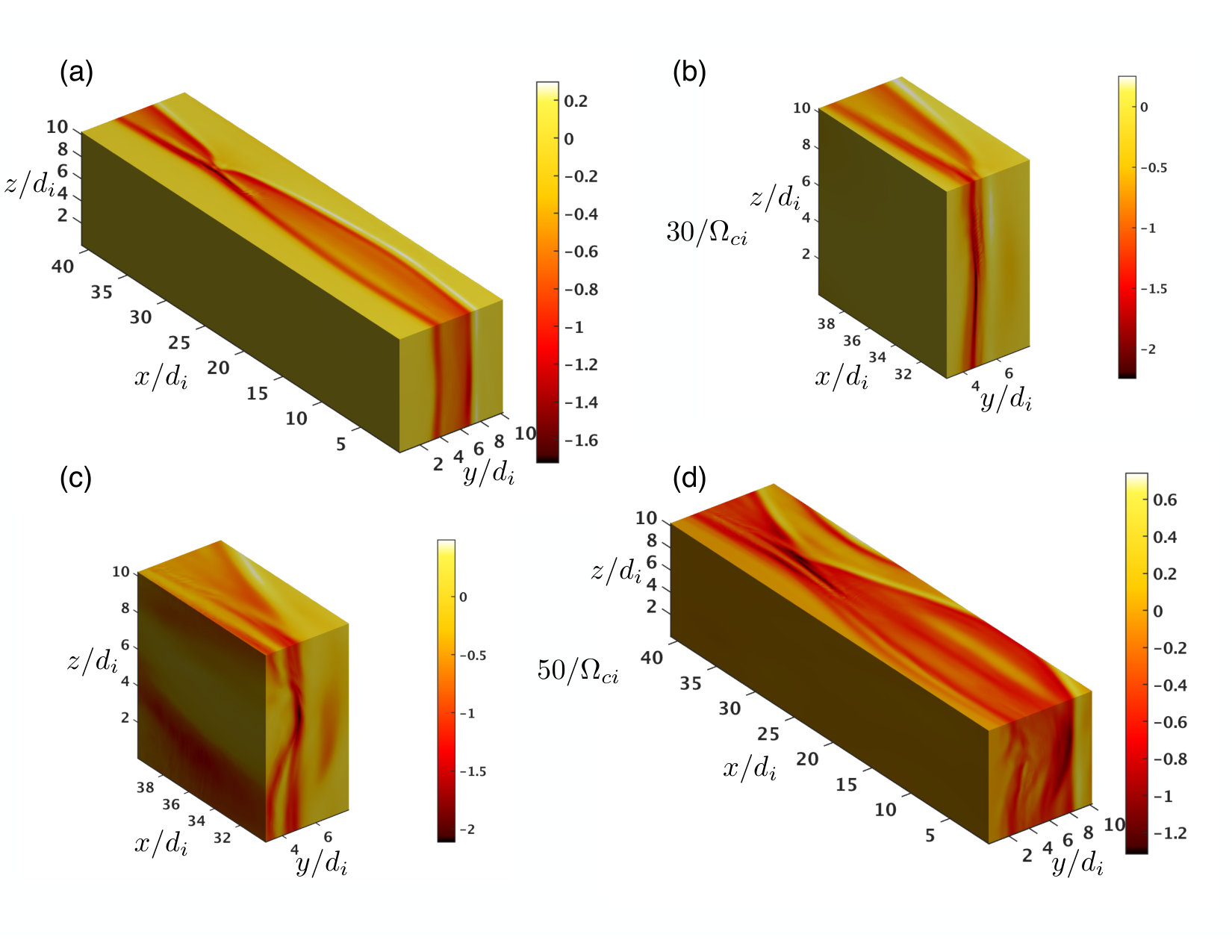 Figure 1
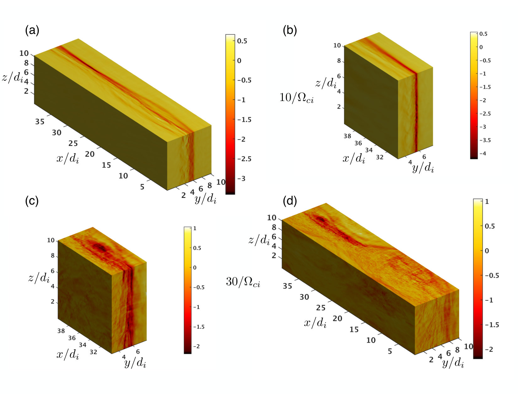 Figure 2
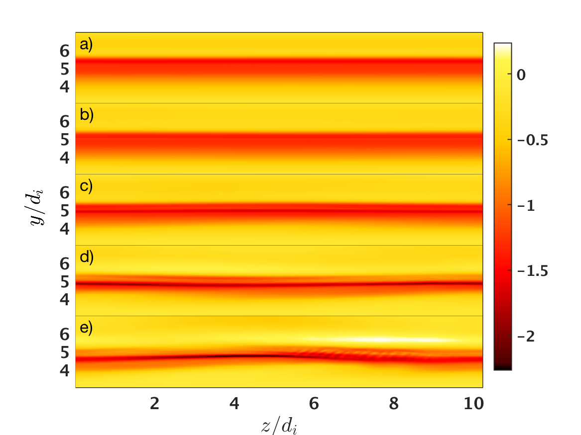 Figure 3
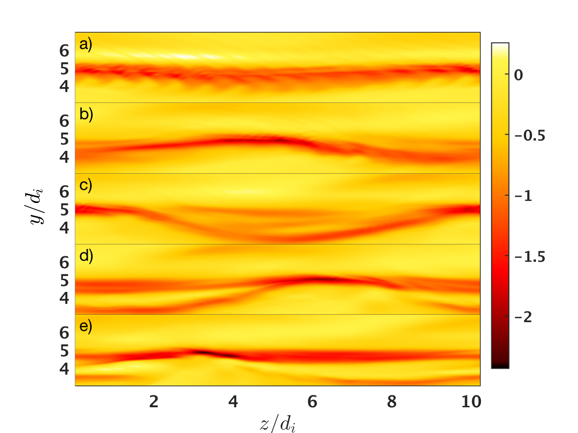 Figure 4
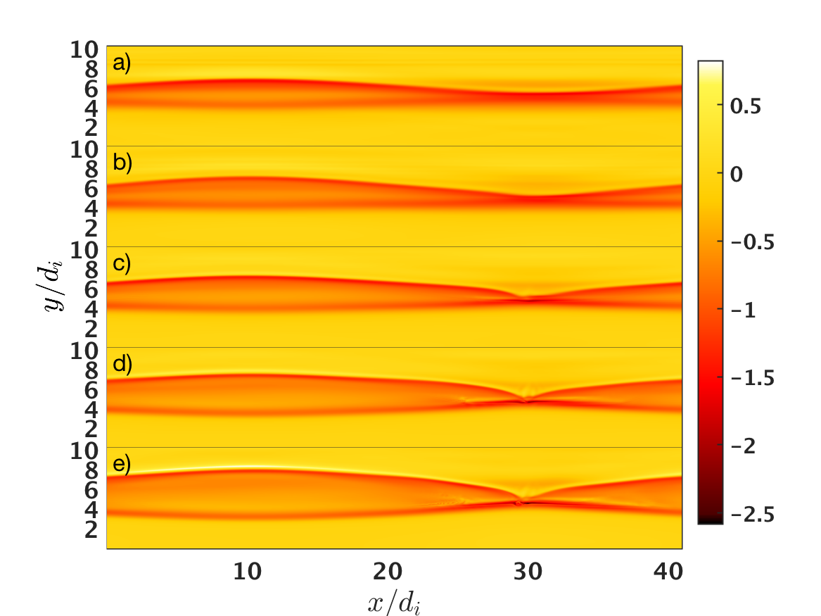 Figure 5
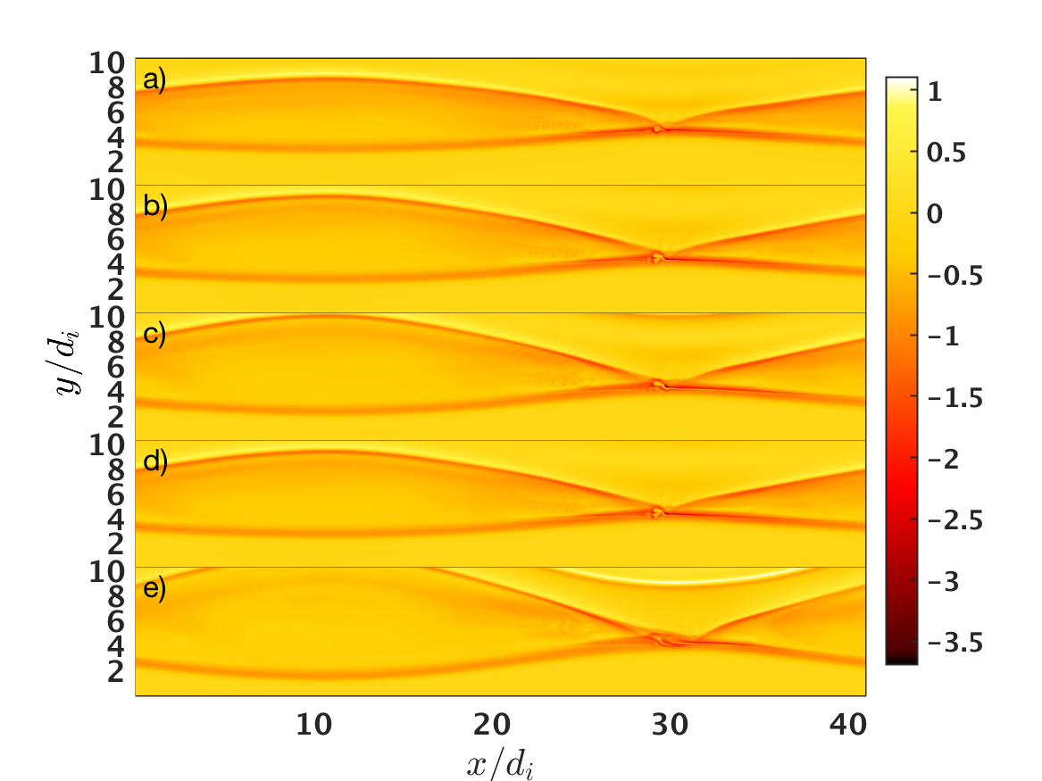 Figure 6
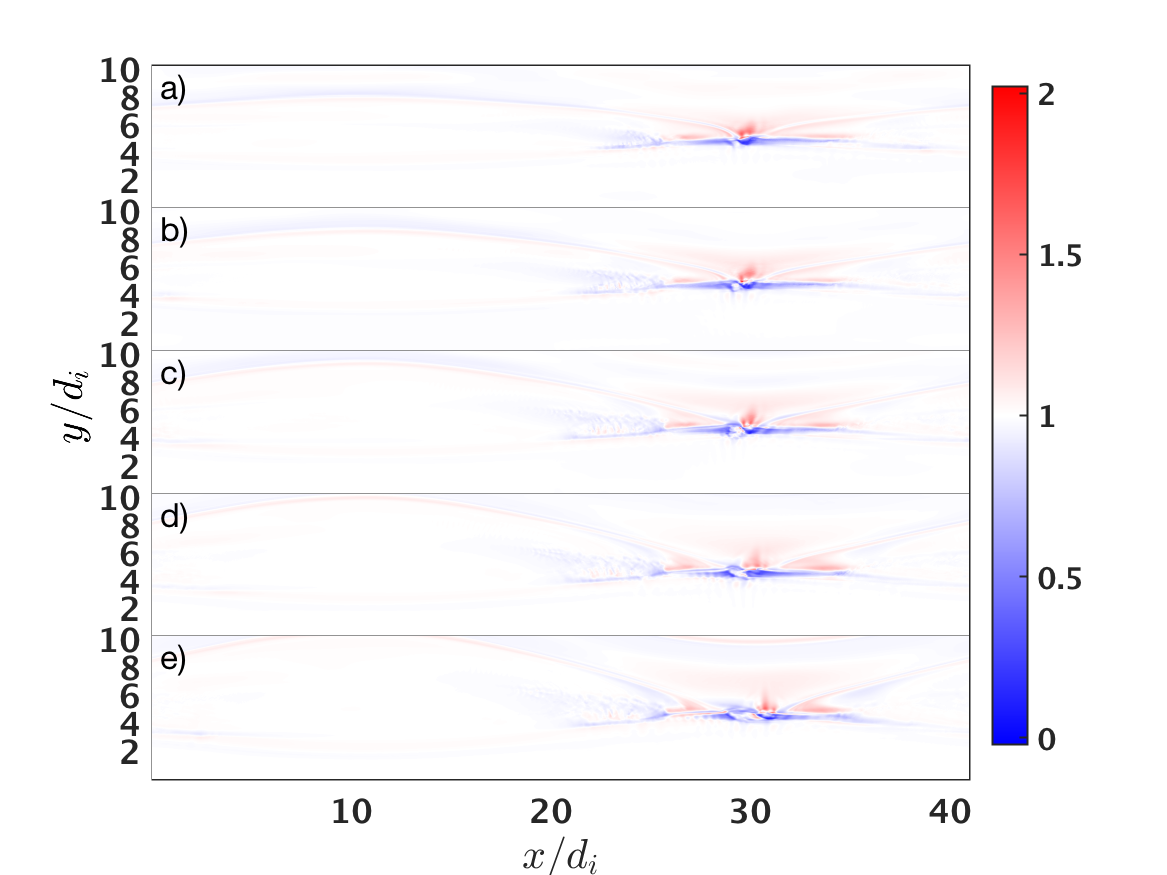 Figure 7
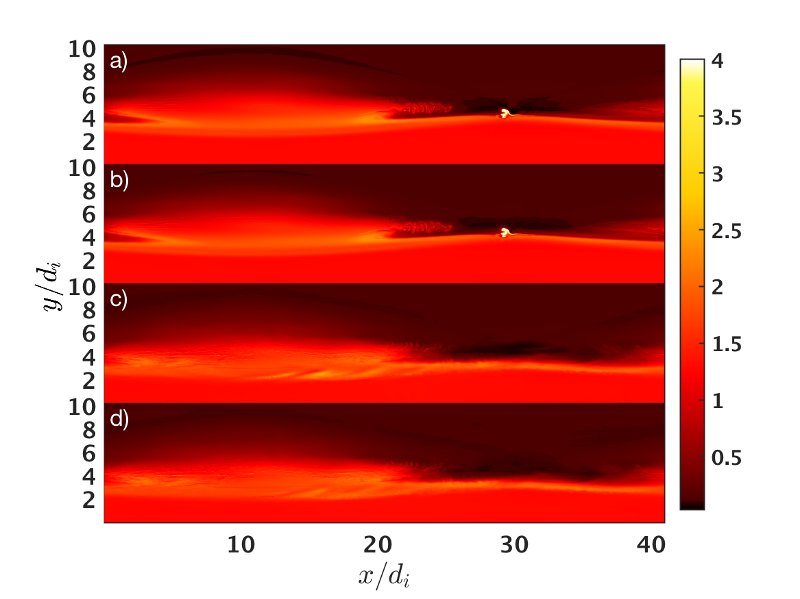 Figure 8
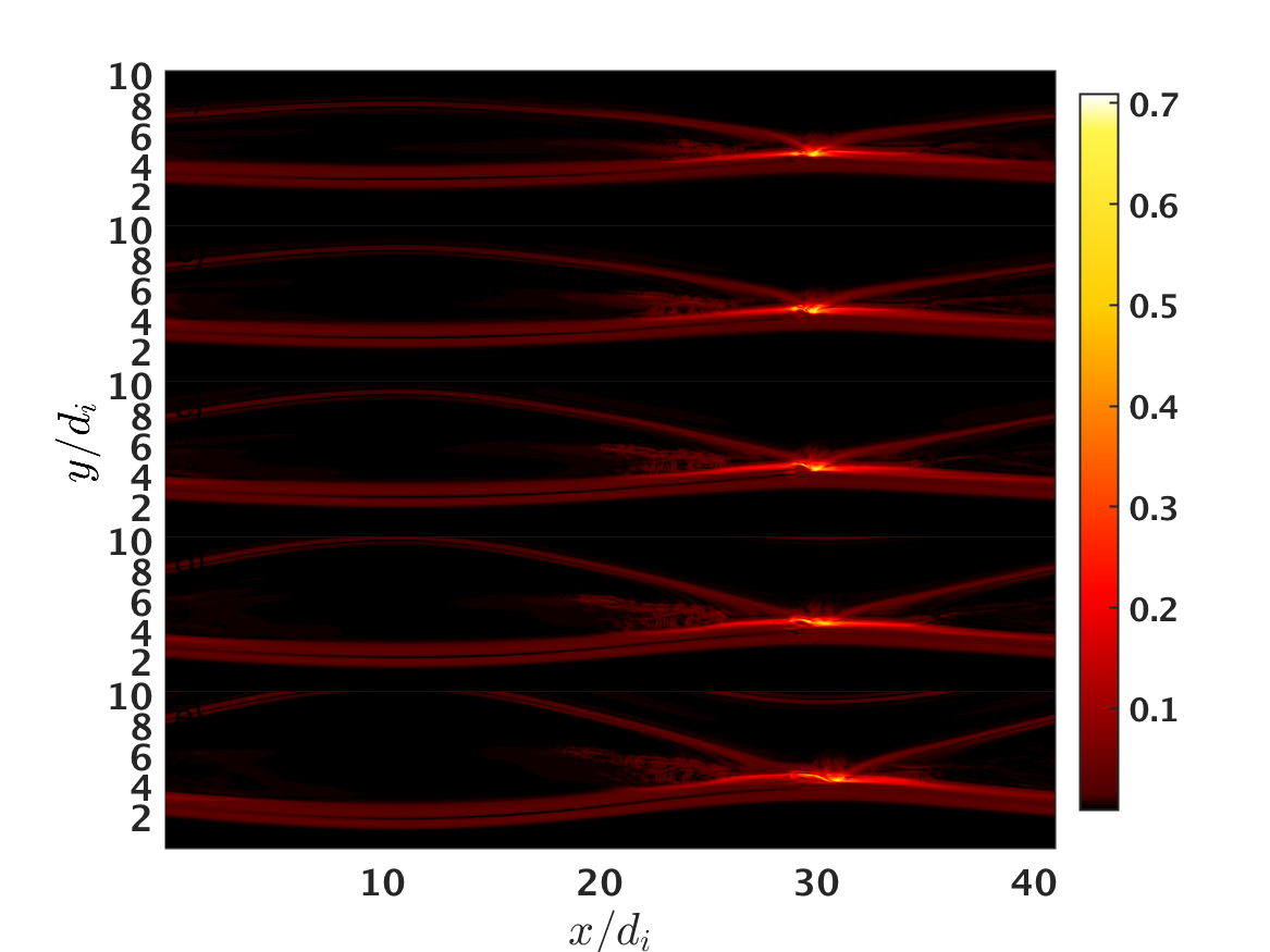 Figure 9
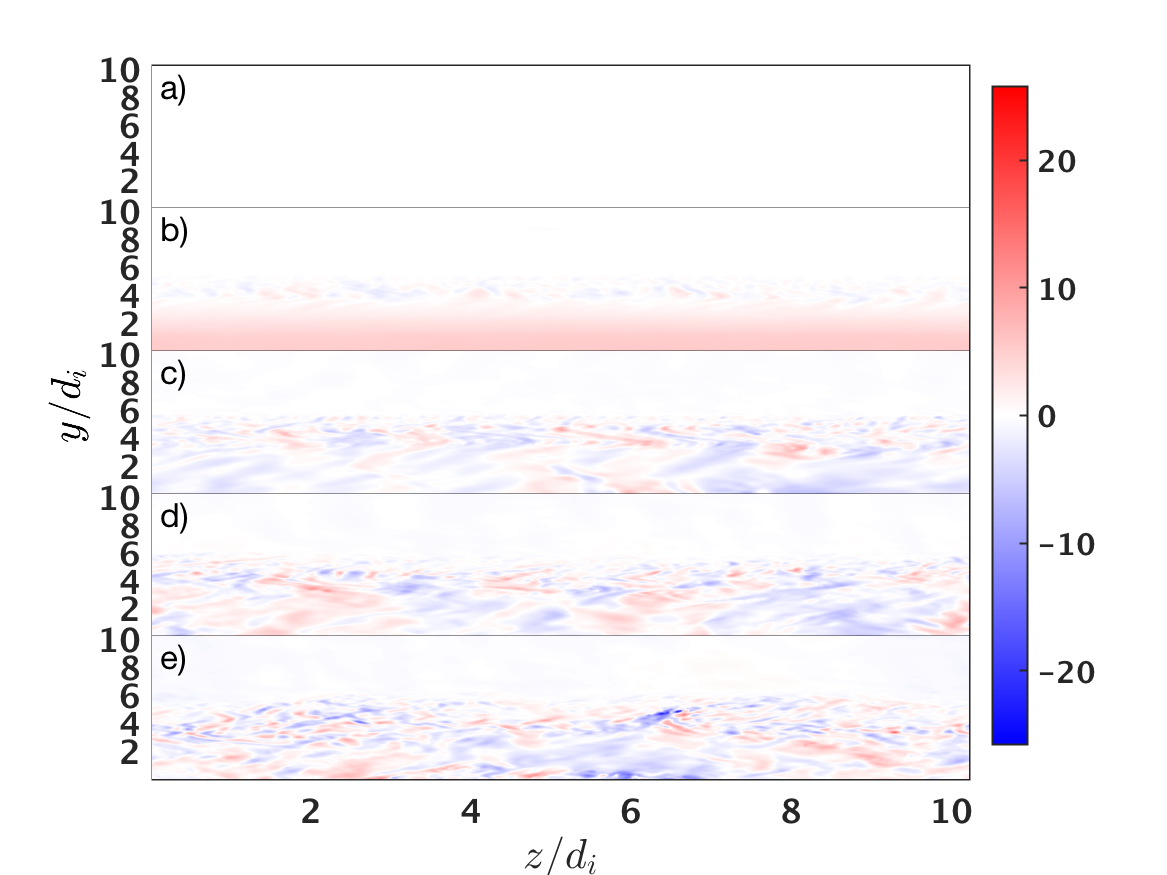 Figure 10
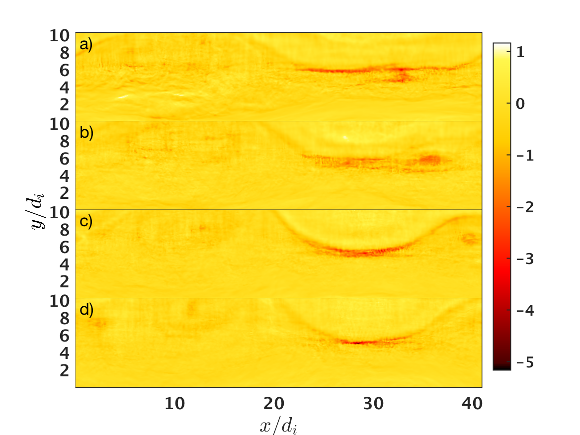 Figure 11
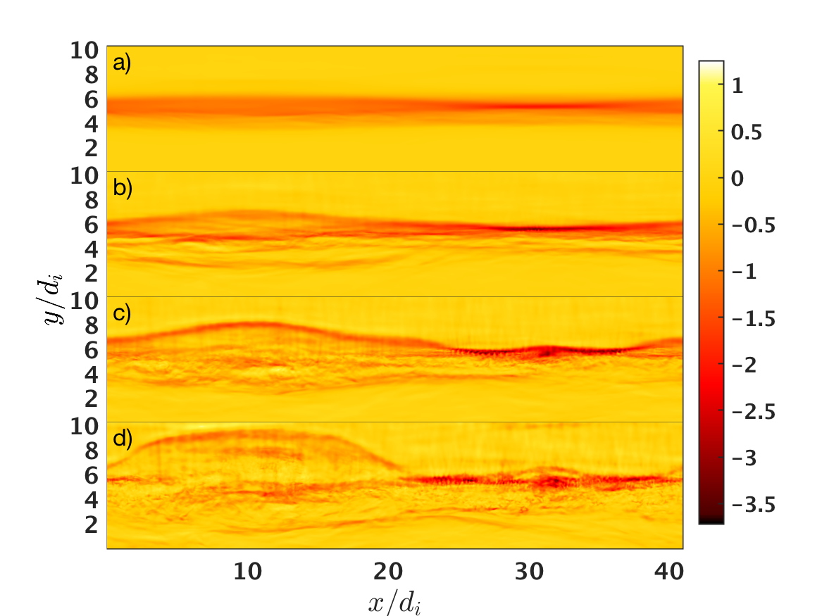 Figure 12
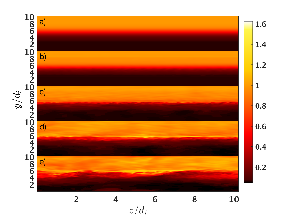 Figure 13
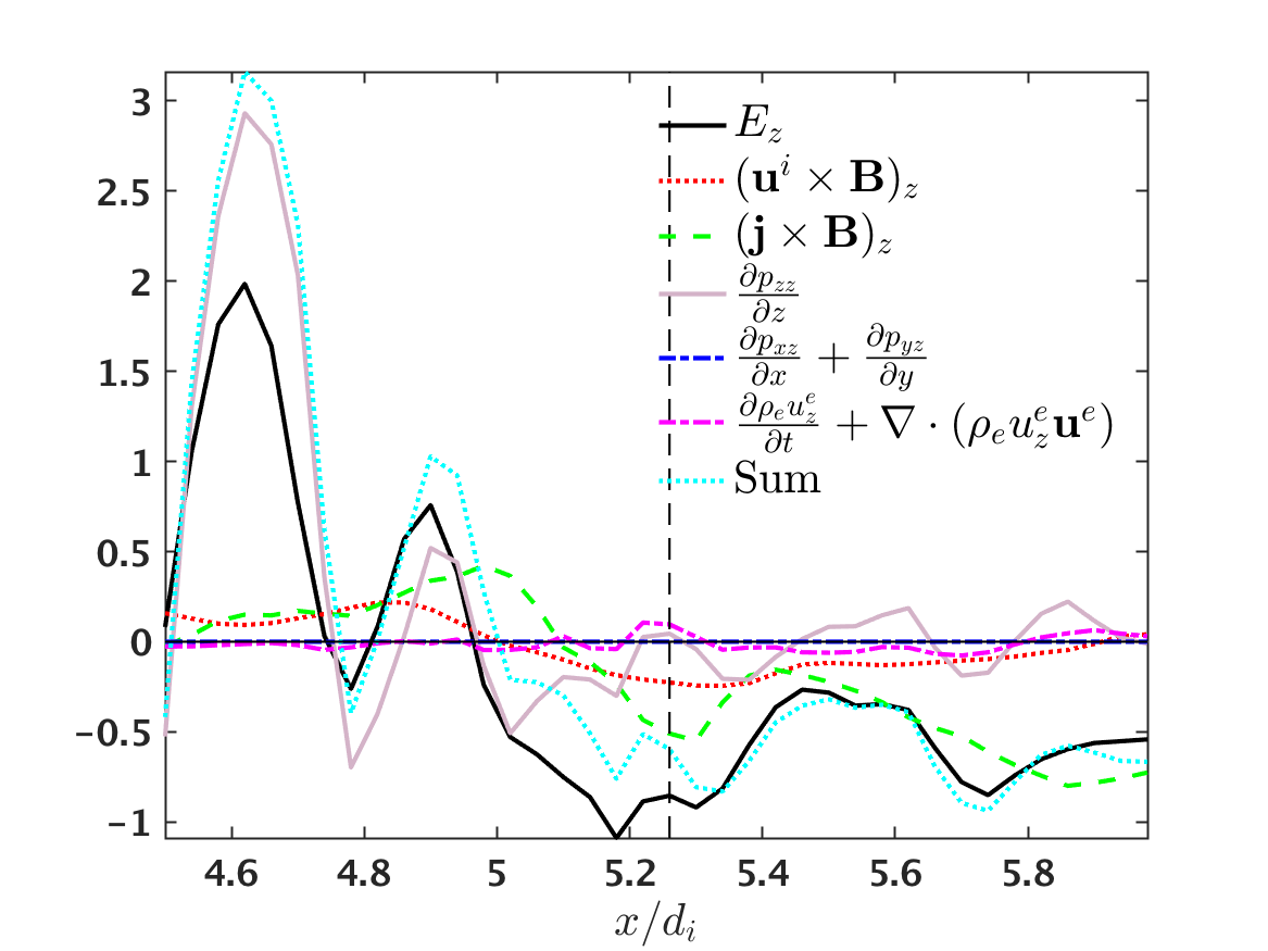 Figure 14
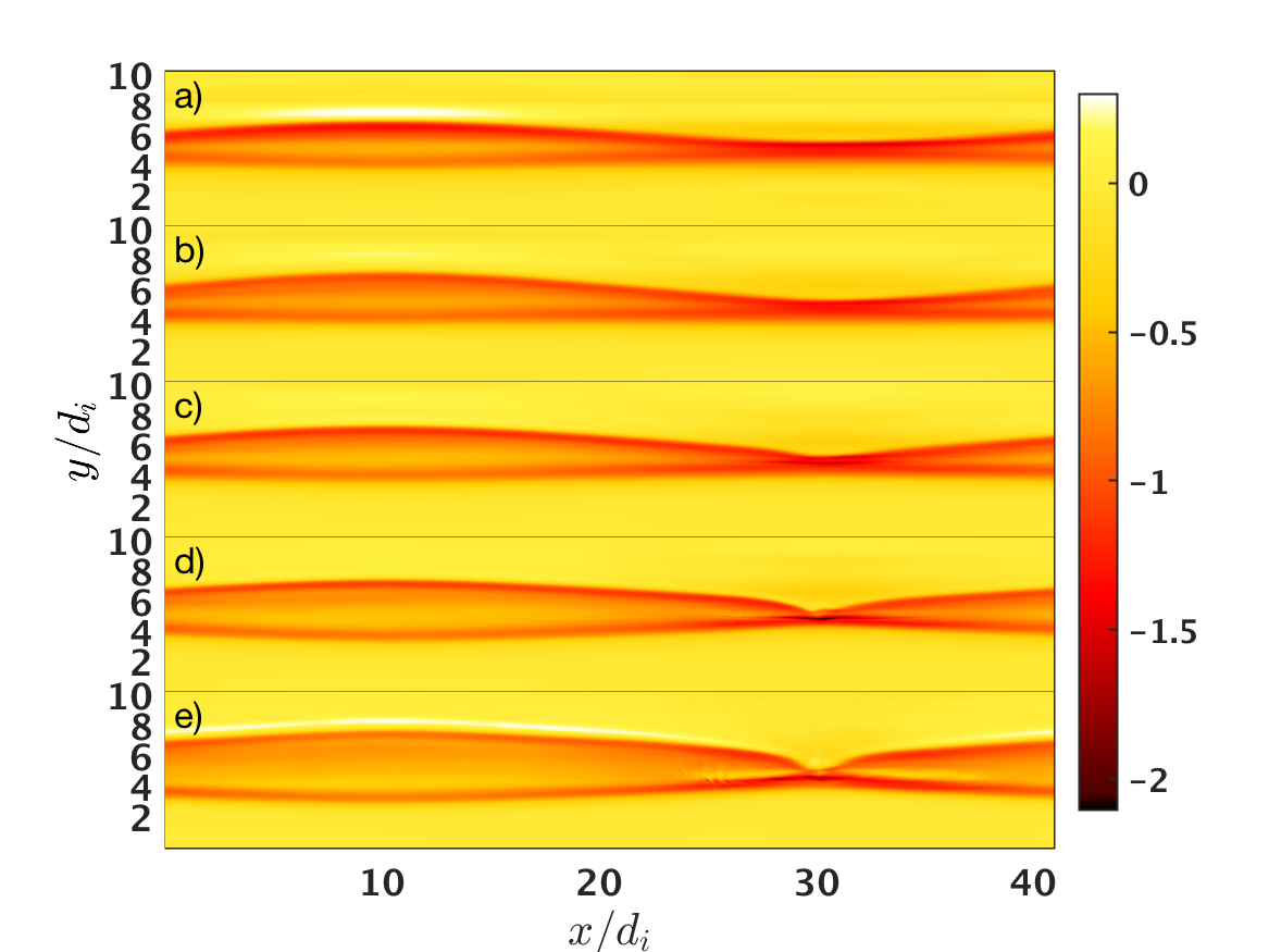 Figure 15
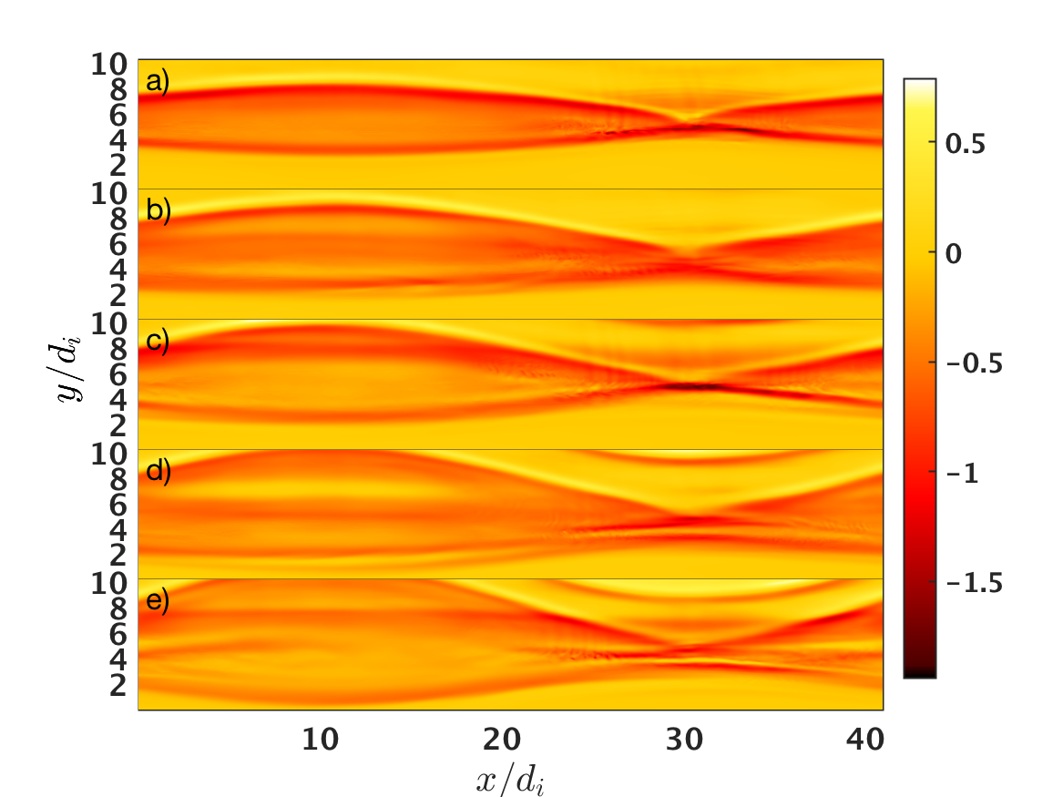 Figure 16
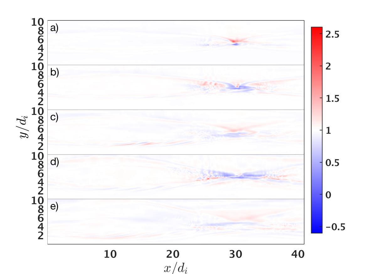 Figure 17
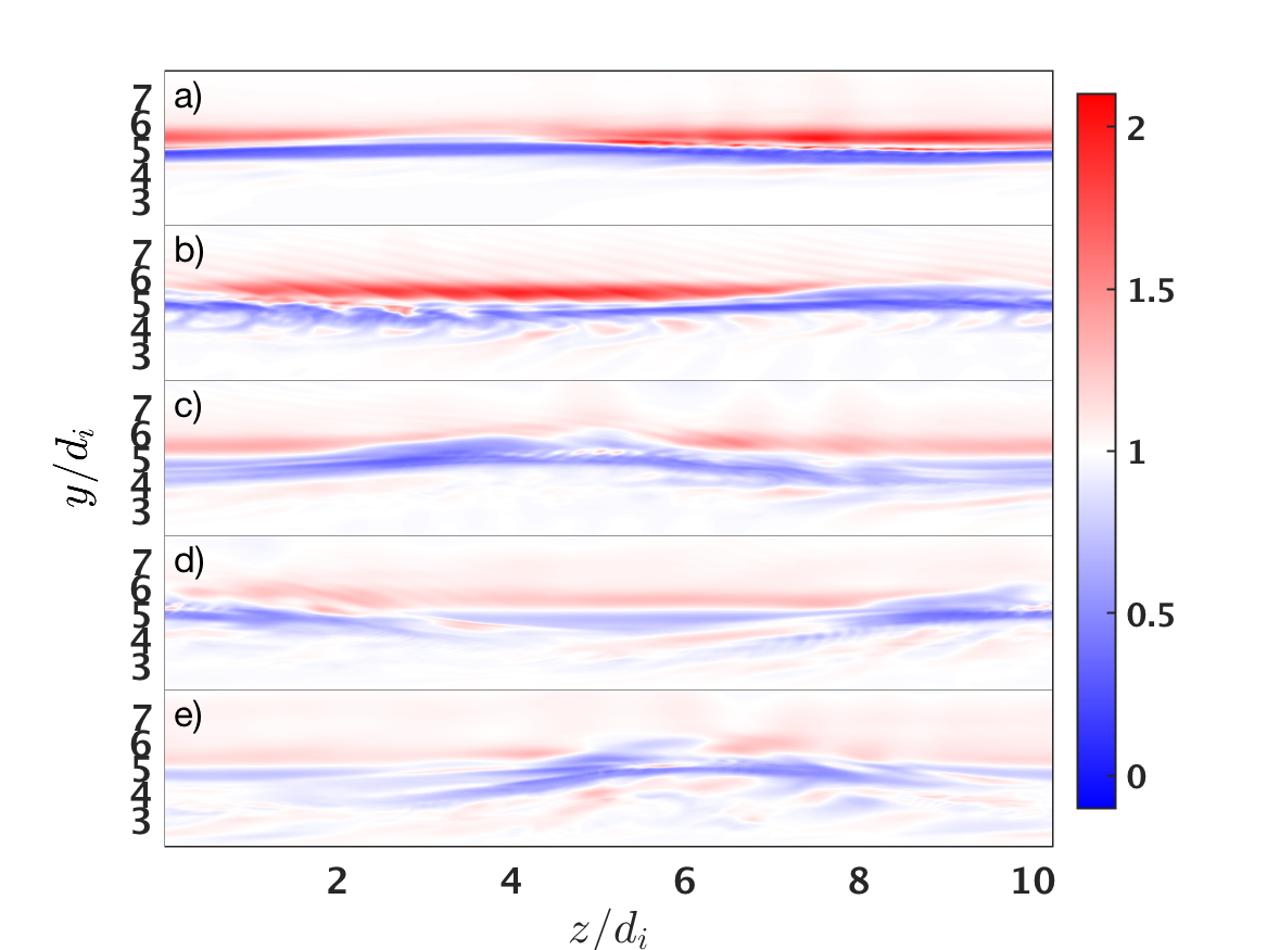 Figure 18
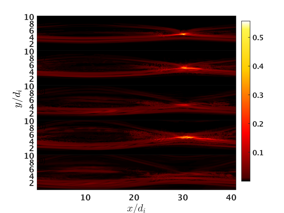 Figure 19
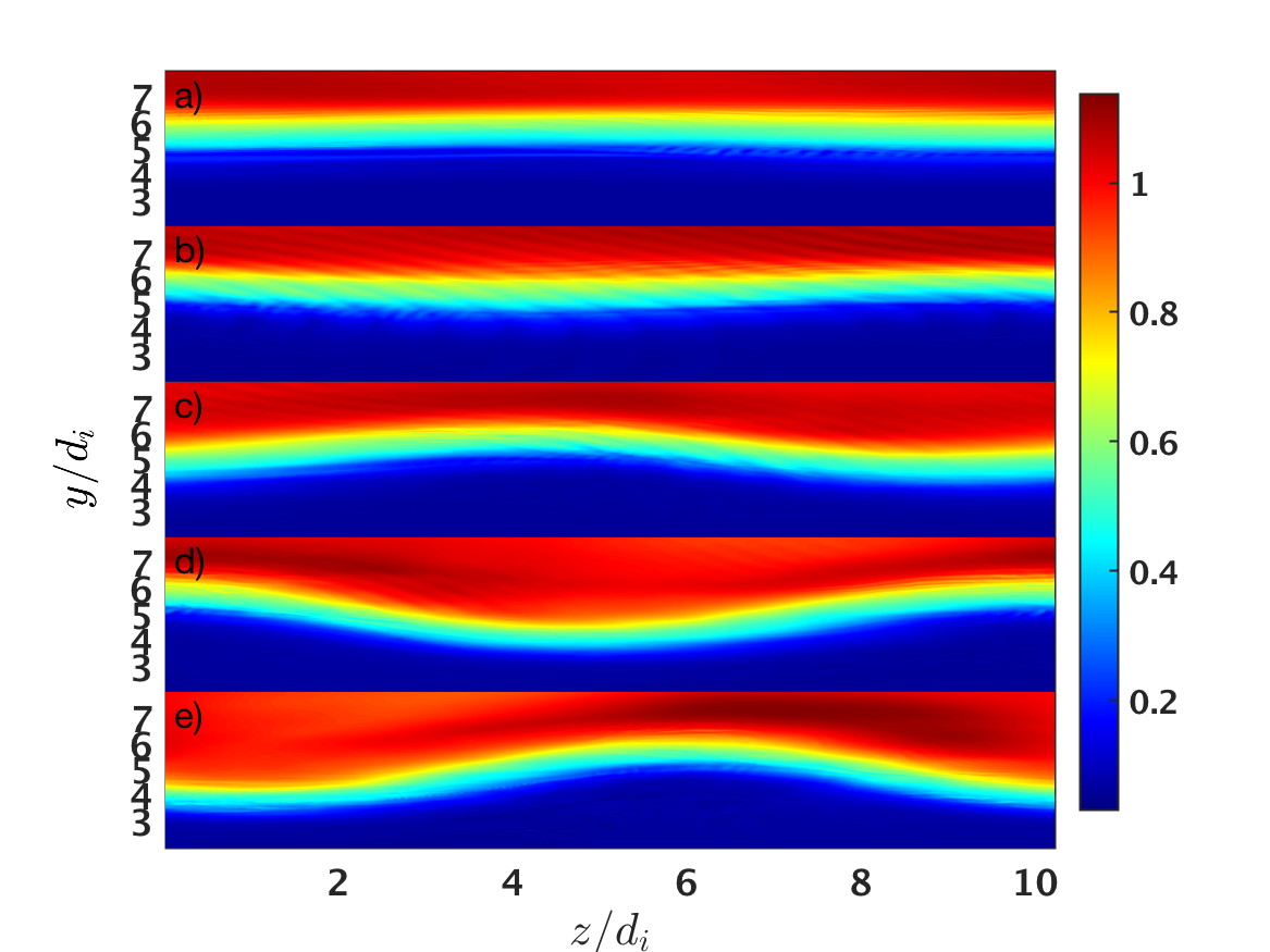 Figure 20
 Figure 21
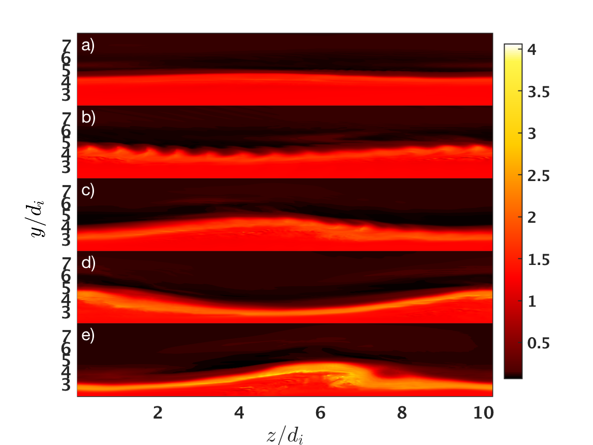 Figure 22
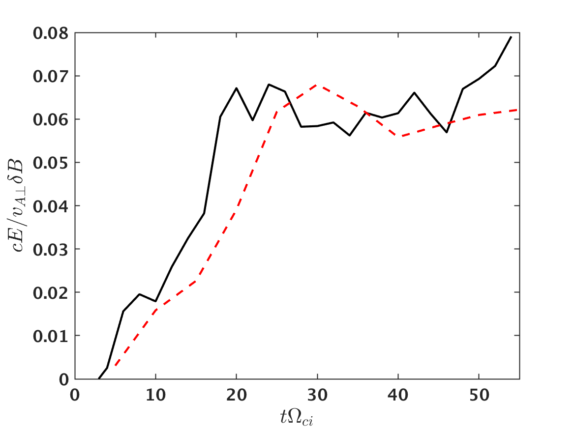 Figure 23
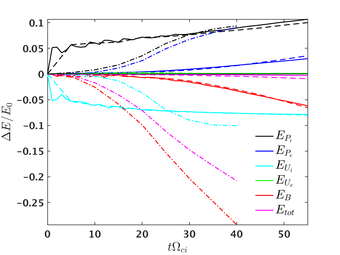 Figure 24
Peer Reviews
No public reviews on file for this paper yet. If you reviewed it on a platform where reviews are public (OpenReview, ICLR, NeurIPS, ICML), you can paste yours below so the community can read it here.
Videos
No videos yet. Explain this paper in a talk, walkthrough, or lecture? Add one.
An extended MHD study of the 16 October 2015 MMS diffusion region crossing
Abstract
The Magnetospheric Multiscale (MMS) mission has given us unprecedented access to high cadence particle and field data of magnetic reconnection at Earth’s magnetopause. MMS first passed very near an X-line on 16 October 2015, the Burch event, and has since observed multiple X-line crossings. Subsequent 3D particle-in-cell (PIC) modeling efforts of and comparison with the Burch event have revealed a host of novel physical insights concerning magnetic reconnection, turbulence induced particle mixing, and secondary instabilities. In this study, we employ the Gkeyll simulation framework to study the Burch event with different classes of extended, multi-fluid magnetohydrodynamics (MHD), including models that incorporate important kinetic effects, such as the electron pressure tensor, with physics-based closure relations designed to capture linear Landau damping. Such fluid modeling approaches are able to capture different levels of kinetic physics in global simulations and are generally less costly than fully kinetic PIC. We focus on the additional physics one can capture with increasing levels of fluid closure refinement via comparison with MMS data and existing PIC simulations.
\draftfalse\journalname
JGR-Space Physics
Department of Astrophysical Sciences, Princeton University, Princeton, NJ, USA. Princeton Center for Heliophysics, Princeton Plasma Physics Laboratory, Princeton, NJ, USA. Department of Astronomy, University of Maryland, College Park, MD, USA. IREAP, University of Maryland, College Park, MD, USA. Princeton Plasma Physics Laboratory, Princeton, NJ, USA.
\correspondingauthor
J. M. [email protected]
{keypoints}
An extended MHD model evolving the full electron pressure tensor and capturing aspects of Landau damping is applied to the MMS Burch event
Many aspects of the fluid model agree well with in situ observations, including strong parallel electron heating near the current layer
The event study demonstrates the efficacy of the ten moment model for global magnetosphere modeling efforts
1 Introduction
The coupled sun-Earth system is a critically important problem for protecting mankind’s technological infrastructure from damaging space weather events, but planetary magnetospheres represent a multi-scale, multi-process physical system that is weakly collisional and coupled to the highly dynamic sun, placing great demand on modeling efforts. Modern in situ spacecraft missions like the Magnetospheric Multiscale (MMS) mission (Burch, Moore\BCBL \BOthers., \APACyear2016) are providing field and particle data at unprecedented temporal and spatial resolution, revolutionizing our understanding of the fundamental plasma processes occurring in Earth’s magnetosphere, such as magnetic reconnection, shocks, and turbulence. Magnetic reconnection of the shocked plasma at Earth’s magnetosheath transports energy from the solar wind plasma into Earth’s magnetosphere (Paschmann \BOthers., \APACyear1979) and is a core process for understanding the sun-Earth coupling.
Despite the impressive quality of in situ measurements, numerical modelling remains our best resource for understanding the global behavior of planetary magnetospheres. Today, the three main numerical approaches are: 1) fully kinetic models such as particle-in-cell (PIC) and continuum Vlasov; 2) hybrid models wherein one species, typically ions, is treated kinetically and the other as a fluid; and 3) fluid models, such as magnetohydrodynamics (MHD), Hall MHD, and various extensions of MHD. Each of these modeling approaches has inherent advantages. For example, fully kinetic models are capable of capturing all of the fundamental plasma physics processes occurring in a magnetosphere; however, such complete modeling comes at the expense of computational complexity, making global simulations of Earth’s magnetosphere too costly to perform. Hybrid approaches are attractive because of their reduced computational cost relative to fully kinetic models, but the electron are typically treated as a massless, isothermal fluid, which is problematic for sub-ion physics such as reconnection, which will be diffused by explicit or numerical resistivity at the simulation grid scale. Additionally, one may be given to assume that since the ions are kinetic, they are treated fully; however, the kinetic ions are coupled to fluid electrons through Maxwell’s equations, which can have consequences at large-scales, such as fast magnetosonic modes being undamped (Parashar \BOthers., \APACyear2014; Grošelj \BOthers., \APACyear2017). Fluid simulations are the most commonly employed approach to model global magnetospheres due to their significantly reduced computational demand, but they assume that the plasma is highly collisional and thus near thermodynamic equilibrium; neither is a good assumption in the weakly collisional plasmas that permeate the solar wind and magnetospheres. Fluid models can be improved by retaining progressively higher fluid moments, with each additional moment retained by the closure corresponding to the fluid model more accurately representing the fully kinetic system. The closure employed by the fluid model can also be tuned to better approximate kinetic effects.
Magnetic reconnection plays a fundamental role in coupling the sun-Earth system; therefore, any fluid model employed in global magnetosphere modeling should minimally capture the physics of reconnection accurately. Reconnection is ultimately controlled by electron demagnetization, which is governed by a combination of electron inertia and pressure agyrotropy (Vasyliunas, \APACyear1975). Based upon this condition, the minimum requirement for a fluid model for global modeling is that the electron closure retain finite mass and evolve the full pressure tensor, implying at least ten moments be retained for each species, , , and , i.e., moments. Since the plasmas of interest are weakly collisional, the closure for a ten moment model should incorporate collisionless effects, such as Landau damping. The Hammett-Perkins Hammett \BBA Perkins (\APACyear1990) approach to closure is one such attempt to incorporate aspects of linear Landau damping in a fluid model. The Hammett-Perkins closure is based upon a linearization of the Vlasov equation, followed by integration over velocity space to obtain an expression for the unclosed fluid moment.
The Gkeyll simulation framework includes both a two-fluid, five-moment model that achieves closure via truncation of moments beyond the isotropic pressure, , and a ten moment model with an approximation of the Hammett-Perkins closure for the heat flux. The ten moment model has been well compared to PIC in the anti-parallel reconnection case (Wang \BOthers., \APACyear2015) and island coalescence (Ng \BOthers., \APACyear2015). Gkeyll has also been successfully employed to model the magnetosphere of the Jovian moon Ganymede (Wang \BOthers., \APACyear2018). To further evaluate the efficacy of the ten moment model, we consider here an asymmetric reconnection event based upon the 16 October 2015 MMS magnetosheath crossing (Burch, Torbert\BCBL \BOthers., \APACyear2016). The large asymmetry of this event provides a stringent test for the ten moment model in the two and three dimensions that can be validated against in situ observations and existing PIC simulations of the event.
The paper is organized as follows. In section 2, we introduce the Gkeyll framework and discuss the closures for the two fluid five (, , and ) and ten moment (, , and ) models that are part of Gkeyll. Section 3 presents the initial conditions derived from the Burch event and the closure parameters chosen for the ten moment model. Simulation results for the ten and five moment models are provided in section 4. Section 5 places the results of the paper in the context of contemporary simulation methods. Finally, in section 6, we present a summary of this paper.
2 The Five- and Ten-Moment Models
The simulation framework we will use for this study is Gkeyll, which includes solvers for continuum Vlasov-Maxwell Juno \BOthers. (\APACyear2018), gyrokinetics Shi \BOthers. (\APACyear2015), and five and ten moment two fluid equations Hakim \BOthers. (\APACyear2006); Hakim (\APACyear2008); Wang \BOthers. (\APACyear2015). In this work, we focus on the five- and ten-moment two-fluid models.
The fluid models evolve the electromagnetic fields through Maxwell’s equations
[TABLE]
[TABLE]
where and are the electric and magnetic field, and are the permeability and permittivity of free space, and , with , , and representing the species charge, density, and velocity. In the following, we drop the species subscripts for notational elegance.
The evolution equations for the moments are obtained via the standard procedure of taking moments of the Vlasov equation:
[TABLE]
[TABLE]
[TABLE]
where is is the completely anti-symmetric Levi-Cevita tensor, which is defined to be for even/odd permutations and zero otherwise, and square brackets around indices represent the minimal sum over permutations of free indices needed to yield completely symmetric tensors.
[TABLE]
is the pressure tensor and
[TABLE]
is the heat-flux tensor, where and are the rest-frame pressure and heat-flux tensors. At this level, the fluid equations are exact but an endless hierarchy, with the th moment requiring knowledge of the st moment.
2.1 The Five-Moment Model
One approach to achieve closure is a simple truncation by neglecting the heat-flux and considering only isotropic pressures. We begin by taking the trace of equation (5) to obtain the exact energy equation
[TABLE]
where
[TABLE]
,
[TABLE]
is the heat-flux vector, is the viscous stress tensor, and is the Kronecker delta function. Closure is obtained by setting and , reducing equation (8) to
[TABLE]
Thus, equations (3)-(4) and (11) constitute a closed system of five-moment equations, , , and , equations for each species. Note that this model reduces formally to Hall MHD in the limit and Srinivasan \BBA Shumlak (\APACyear2011).
2.2 The Ten-Moment Model
To retain additional kinetic physics relative to the five-moment model, we desire the full pressure tensor, thus constituting a ten moment model. Therefore, we must obtain an expression for appearing implicitly in equation (5) to close the system. Additionally, since space plasmas tend to be weakly collisional, we seek a collisionless closure and thus choose to use a Hammett-Perkins Hammett \BBA Perkins (\APACyear1990) inspired closure. The closure is based upon a linearization of the Vlasov equation, followed by integration over velocity space to obtain an expression for the unclosed fluid moment, which in this case is the heat flux. This approach leads to expressions involving plasma response functions in Fourier space, which are approximated by an -pole Padé approximant. Following Hammett \BBA Perkins (\APACyear1990), we choose to employ a -pole approximation to the response function; however, since the approximation is in Fourier space, the closure is non-local along magnetic field lines. To reduce the computation demand of integrating along field lines and Fourier transforming, we further use a local approximation of the heat-flux divergence
[TABLE]
where is the thermal speed, and is a typical wavenumber, which defines a scale below which collisionless damping is thought to occur. Equation (12) together with equations (3)-(5) represent the closed ten moment model for , , and . Note that this closure closely resembles a collisional closure that scatters the system towards isotropy with collision frequency . would allow the pressure to evolve freely, while the limit isotropizes the pressure tensor at all scales, approaching the five-moment limit.
3 Initial Conditions
The initial conditions for the study contained herein are motivated by the first observed Magnetospheric Multiscale (MMS) spacecraft crossing of a magnetic field X-line at Earth’s magnetosheath Burch, Torbert\BCBL \BOthers. (\APACyear2016), hereafter referred to as the Burch event. The initial magnetic field and temperature profiles have the following form,
[TABLE]
where subscripts and correspond to magnetosheath and magnetosphere quantities, is the initial current sheet width, is the asymptotic ion inertial length on the sheath side, and is the sheath ion plasma frequency. For notational simplicity, we will use and going forward, where is the sheath gyrofrequency. The initial magnetic field profile is given by , where , with a uniform guide field . The initial electron and ion temperature profiles are also given by equation (13) and satisfy and . The density profile is chosen to satisfy force balance across the sheet, which leads to . An initial vector potential perturbation of the form
[TABLE]
is added to initiate reconnection, where . The simulation dimensions are in 2D and in 3D, with fully periodic boundary conditions in all cases. The number of grid points are and giving and in 2 and 3D. A reduced mass ratio of and are used in all cases, where is the asymptotic sheath Alfvén speed based upon the reconnecting field. To break the inherent symmetry of the initial conditions in 3D, noise with root-mean-square amplitude is added to the first 20 Fourier modes in the , , and directions of and . We will refer to the 2D ten moment and 3D five and ten moment Gkeyll simulations as 2D10, 3D5, and 3D10, respectively.
Prior Gkeyll reconnection studies (Ng \BOthers., \APACyear2015; Wang \BOthers., \APACyear2015) have demonstrated that is required to achieve agreement with particle-in-cell simulations, where subscript refers to species. However, a value of provides slightly better performance for turbulence simulations without significantly degrading the reconnection performance (Juno \BOthers., \APACyear2018). Since we expect these event simulations to be turbulent, we choose closure parameters for both ten moment model simulations to be . Formally, this choice for will permit pressure anisotropy and agyrotropy to develop to a scale before the ten moment closure scatters the pressure toward isotropy.
4 Results
4.1 Ten-Moment Simulation Results
We first present the results of the Burch event study using the ten-moment model in two and three dimensions. In figure 1 is presented the reconnection rates (left panel) and relative changes of energy components (right) for runs 2D10 (solid) and 3D10 (dashed). The reconnection rate in the 3D case was computed by averaging and over the -direction and integrating to construct an average vector potential, . In both 2 and 3D, the rate reaches a plateau at the canonically observed value of . The relative change of the energies is essentially identical in 2D and 3D for the ten-moment model. Thus, in terms of energy exchange and reconnection rates, the 2 and 3D ten-moment simulations are fundamentally similar.
The evolution of the out-of-plane current density, , in the -plane for runs 2D10 and 3D10 are presented in figures 2 and 3. For run 3D10, the current density is taken at . The early-time evolution for to in increments is presented in the left panel of each figure. Little qualitative or quantitative difference exists during this phase, the most significant difference being a moderately increased current density in 2D due to the existence of sharper magnetic field gradients. The right panels of the figures presents the current density at times to . Beginning at , the 2 and 3D evolution noticeably diverges. The source of the divergence becomes clear by examining the full 3D evolution of the current in run 3D10, as shown in figure 4. At the current layer is predominantly laminar, while at , the entire layer has become turbulent. In figure 5 is shown the current in the -plane at the X-line, , at the same times as figure 3. It is clear that in three dimensions turbulence plays an active role, broadening the current layers, thereby further reducing the local current density. The entire current layer is also kink unstable with wavelength equal to the longest wavelength accessible in the domain.
The turbulence is generated by a field aligned shear flow instability with wavelength (Romero \BOthers., \APACyear1992). Figure 6 presents slices of the electron density (left) and temperature (right) at the X-line at times prior to and following the growth of the instability, to . The instability drives a low amplitude density perturbation along the current layer that spreads into the high density, magnetosheath, side. By using the large temperature gradient across the layer as a tracer in the right panel of figure 6, it becomes apparent that the instability drives Kelvin-Helmholtz like vorticies along the current layer that lead to enhanced mixing relative to the 2D simulation. This instability is active along the entire separatrix layer; however, it is most significant in the vicinity of the X-line.
The electron shear flow instability present in run 3D10 has been observed in PIC simulations of the Burch event (Le \BOthers., \APACyear2017); however, the shear instability is preceded by the growth of the lower hybrid drift instability (LHDI) (Krall \BBA Liewer, \APACyear1971; Daughton, \APACyear2003), which feeds off of the large density gradient present in this event, but the LHDI is absent from this ten-moment simulation. Prior particle-in-cell simulations of the Burch event (Price \BOthers., \APACyear2016; Le \BOthers., \APACyear2017) find that the LHDI plays a fundamental role in generating turbulence that both supports the reconnection electric field and enhances mixing and electron heating. Linear analysis of the ten-moment model performed in Ng \BOthers. (\APACyear2019) shows that the LHDI is indeed captured by the model, but the closure parameter for both species, , can significantly modify the growth rate of the instability. To recover kinetic growth rates, the ion closure parameter must be approximately equal to the wavelength of the fastest growing LHDI mode. Unfortunately, the fastest growing LHDI modes have (Daughton, \APACyear2003), which differs significantly from the closure parameter that is necessary to model reconnection in the vicinity of the X-line, , and the value chosen for this study. Therefore, the ten-moment closure for the parameters employed in run 3D10 damps the LHDI, leading to a growth rate that is reduced by approximately an order of magnitude relative to kinetic theory.
The electron temperature anisotropy, , for runs 2D10 (left) and 3D10 (right) are presented in figure 7 for times to . Significant electron temperature anisotropy develops in both two and three dimensions in the ten-moment model; however, the presence of shear driven turbulence and mixing in three dimensions enhances the temperature anisotropy along the separatrices and significantly broadens the region with in the vicinity of the X-line. Examining the structure of the temperature anisotropy in the -plane in the left panel of figure 8 for run 3D10 reveals that the most significant excess parallel heating occurs in regions where the current layer has oscillated toward the magnetosphere, creating local depressions of the magnetic field amplitude.
The largest value of the temperature anisotropy occurs in run 3D10 and is , which is in close agreement with the value observed by MMS [see figure 3I of Burch, Torbert\BCBL \BOthers. (\APACyear2016)]. However, the Burch event observation of is entirely on the low density, magnetosphere side of the current layer, and the magnetosheath is observed to be nearly isotropic. In both runs 3D10 and and 2D10, is only generated on the magnetosheath side of the X-line, while the magnetosphere side is predominantly plasma. The right panel of figure 8 presents electron (a & c) and (b & d) separately for runs 2D10 (a & b) and 3D10 (c & d) at and . Overall, the electron heating is isotropic, with regions of anisotropic heating being due to isolated and small variations in the temperature components. Three dimensional PIC simulations of the Burch event find that the entire magnetosphere separatrix layer is heated in only the parallel direction with [see figure 3 of Le \BOthers. (\APACyear2017)], which is consistent with the location but not magnitude of observed temperature anisotropy in the MMS event. The anisotropic heating in the 3D PIC result is attributed to mixing induced by the LHDI, which is only present in three dimensions; however, as noted above, the LHDI is damped in the ten-moment model.
Since the ten-moment model evolves the full pressure tensor, we present in figure 9 the electron pressure agyrotropy for runs 2D10 (left) and 3D10 (right), where
[TABLE]
is the measure of gyrotropy defined in Swisdak (\APACyear2016). By definition, , where corresponds to gyrotropy (maximal agyrotropy). The peak values of and occur in the vicinity of the X-point and X-Line in 2 and 3D, respectively, with the reduced peak value in run 3D10 due to turbulence broadening the current layers. The gyrotropy measure also highlights the separatricies, where . The structure and magnitude of are generally consistent with results observed in PIC simulations and in situ spacecraft observations of reconnection, e.g., Swisdak (\APACyear2016); Zenitani \BBA Nagai (\APACyear2016); Bourdin (\APACyear2017); Genestreti \BOthers. (\APACyear2018).
To further emphasize the importance of the pressure agyrotropy at the X-line, we next examine the components of the generalized Ohm’s law for the ten-moment model, which can be derived from the electron momentum equation, equation (4). At the X-line, only the guide field, , aligned component of the Ohm’s law contributes
[TABLE]
where is the charge of an electron and is the electron mass density. The one dimensional components of the generalized Ohm’s law across the current layer for run 3D10 at time and are plotted in the left panel of figure 10, where the vertical dashed line indicates the location of the magnetic field reversal. The only component of the Ohm’s law that contributes significantly at the reversal is the off-diagonal pressure tensor (dot dashed blue). Away from the X-line, the Hall term, , (dashed green) is the primary contributor.
4.2 Five-moment Simulation Results
Moving to the five-moment model, we begin by examining the relative change in energy for run 3D5 presented in the right panel of figure 1 as dash-dotted lines. The evolution of run 3D5 is notably different from the ten-moment simulations, with the magnetic field decaying rapidly, and its free energy going to ion and electron thermal energy. Also notable is the poor conservation of total energy (magenta) in this run that onsets shortly following the initial decay of magnetic energy. Poor conservation of energy indicates that a significant amount of energy is reaching the grid scale, even at this early stage of the simulation. The reconnection rate for run 3D5 is not plotted in this figure for reasons that will become apparent below.
In figure 11 is plotted the evolution of the out-of-plane current density taken at for run 3D5 at times to (left) and to (right), with each frame separated by . The full three dimensional structure of the layer at times and are presented in figure 12. Clearly, the behavior of the five-moment model for these highly asymmetric parameters differs significantly from that of the ten-moment model. The current layer is permeated by turbulence, which leads to substantial diffusion and broadening across the entire layer, essentially destroying the current layer. By , the entire domain has become turbulent. The strong turbulence present in this simulation is responsible for the transport of energy to the grid scale that results in poor energy conservation. Additionally, the turbulence precludes one from reliably calculating the reconnection rate using conventional methods, since the magnetic X and O points are ambiguous.
The origin of the turbulence in this simulation is the LHDI, in stark contrast to the ten-moment results. Evidence for this can be seen in figure 13, where the evolution of the electron density (left) and (right) are plotted in the -plane at times to . Already, at , evidence of the LHDI has become apparent, with density and electric field fluctuations extending from the the edge of the central current layer into the low density, magnetosphere, side with wavelength . By , the initially electrostatic modes have fully penetrated the current layer and fill the entire magnetosphere side.
These results concerning the LHDI are also supported by linear stability analysis of the five-moment model presented in Ng \BOthers. (\APACyear2019). Ng \BOthers. (\APACyear2019) demonstrates that the LHDI grows by a factor of two to three faster in the five-moment model than in kinetic theory, thus leading to the explosive growth of the instability and subsequent turbulence seen in run 3D5.
The generalized Ohm’s for the five-moment model differs from that for ten-moment model given in equation (16) only in that the the off-diagonal pressure tensor components do not contribute. The one dimensional components of the generalized Ohm’s law across the current layer for run 3D5 at time and are plotted in the right panel of figure 10, where the vertical dashed line indicates the location of the magnetic field reversal. The primary contributor to the reconnection electric field at the X-line is the Hall term (dashed green). Away from the X-line, the electron pressure gradient (lavender) is the primary contributor.
5 Discussion
The ten-moment model presented in section 2.2 represents the most sophisticated fluid closure available that is numerically tractable for global magnetosphere modeling. The closure employed by the ten-moment model captures many aspects of kinetic theory that are well beyond the capabilities of the most commonly applied model to global magnetospheres, MHD. MHD assumes the plasma is highly collisional, such that it is in local thermodynamic equilibrium; therefore, the only mechanism available to break field lines and allow magnetic reconnection to proceed is resistivity, be it grid-scale diffusion or explicitly imposed. In either case, the resistivity employed exceeds the real value in weakly collisional planetary magnetospheres by orders of magnitude, thus altering significantly the location, evolution, and transport induced by reconnection. Indeed, MHD models predict either extended Sweet-Parker layers or copious plasmoid production, with the evolution being determined entirely by the Lundquist number rather than kinetic processes (Daughton \BBA Roytershteyn, \APACyear2012). Additionally, although the ten-moment model has difficulty capturing the LHDI, the LHDI is completely ordered out of MHD.
Fluid models more sophisticated than MHD exist, such as Hall MHD or two-fluid models with isothermal closures, but they are rarely employed in the context of global modelling due to computational constraints. However, both Hall MHD and traditional two-fluid models also neglect the electron kinetic effects that permit reconnection to proceed naturally, relying on resistivity to break field lines. As demonstrated by the five-moment model in section 4.2, retaining finite electron inertia effects without fully evolving the pressure tensor can lead to anomalously large growth rates for instabilities that are common to global magnetospheres, such as the LHDI.
As computational resources are expanding, hybrid approaches are gaining increased focus, because they treat the ions kinetically; however, hybrid models suffer many of the same issues outlined above. Since the electrons are treated as a fluid, they also require a closure model, which is that of a massless, isothermal fluid, although finite electron mass is occasionally retained. Therefore, reconnection still proceeds via resistivity, despite having fully kinetic ions. The electron closure also feeds back on the ions through Maxwell’s equations, leading to consequences at large-scales, such as undamped fast magnetosonic modes (Grošelj \BOthers., \APACyear2017) and electron equation of state dependent energy transport (Parashar \BOthers., \APACyear2014). Further, electron instabilities such as the LHDI remain problematic in hybrid models, because they occur on electron kinetic scales and often involve electron phase space resonances.
Despite the overall success of the application of the ten-moment model to the Burch event presented in Section 4.1, it does display some weaknesses relative to fully kinetic, particle-in-cell simulations. Specifically, the ten-moment closure fails to properly capture the LHDI and the important role it plays in heating and transporting plasma across the separatrix. The source of the disagreement follows directly from the local closure chosen in section 2.2. Ng \BOthers. (\APACyear2019) demonstrates that a non-local heat flux closure is able to accurately recreate the LHDI, where the local heat flux closure presented in equation (12) is replaced with
[TABLE]
where , represents the Fourier transform, and is an adjustable constant. The factor appearing in the denominator makes this closure non-local in real space, drastically increasing the computational expense and making its utility for global modelling limited. A gradient-based closure to the ten-moment model has been introduced by Allmann-Rahn \BOthers. (\APACyear2018), where equation (12) is replaced with
[TABLE]
and is an adjustable constant. Allmann-Rahn \BOthers. (\APACyear2018) find that the gradient closure better agrees with Vlasov and PIC simulations than the local closure presented in equation (12), with minimal additional computational expense for typical choices of . Therefore, the gradient closure appears to be a good alternative to the local closure for global modelling, but further study to determine how well the gradient closure captures the LHDI is necessary.
6 Summary and Conclusions
We have performed an event study of the Burch, Torbert\BCBL \BOthers. (\APACyear2016) 16 October 2015 MMS diffusion region crossing using the two-fluid, multi-moment models contained in the Gkeyll framework. The ten-moment model evolves the full pressure tensor and is closed with a local Hammett-Perkins model for the heat flux divergence. The closure is designed to capture linear Landau damping that sets in at a fixed, isotropic, and species dependent wavenumber, . The five-moment model achieves closure by truncating the moment hierarchy at the isotropic pressure for each species, setting all higher moments to zero. The ten-moment model was applied to the Burch event in two and three dimensions, while the five-moment model was applied only in three dimensions.
The ten-moment model was found to accurately capture aspects of the Burch event that are beyond the capabilities of conventional fluid approaches, such as MHD, Hall MHD, or two-fluid models with isothermal closures. Inclusion of the full electron pressure tensor, electron inertia, and Hall terms permits the electrons to demagnetize naturally at the X-line. The pressure agyrotropy structure and amplitude developed by the ten-moment model is consistent with existing PIC simulations of reconnection. The ten-moment model also accurately reproduces the same magnitude of electron temperature anisotropy as observed in situ with MMS. However, the spatial location of the temperature anisotropy is on the magnetosheath side of the X-line; whereas, in situ observations (Burch, Torbert\BCBL \BOthers., \APACyear2016) and PIC simulations (Le \BOthers., \APACyear2017) find it to be on the low density, magnetosphere side. The discrepancy is due to lower hybrid drift instability (LHDI) induced heating and transport in the PIC simulation. The chosen closure parameter for the ion ten-moment model, , is too far in scale from the fastest growing LHDI mode and is thus anomalously damped. Choosing a larger value for the closure parameter, , can reproduce the growth of the LHDI accurately but would prevent reconnection from proceeding correctly, since the electron pressure would be scattered toward isotropy at a much faster rate, precluding electron agyrotropy from forming. Electron shear flow and kink instabilities do develop in the layer in three dimensional ten-moment Gkeyll simulation, which are also observed in PIC simulations (Le \BOthers., \APACyear2017). The shear flow instability generates significant turbulence and increases the transport across the current layer relative to the two dimensional Gkeyll simulations of the Burch event.
In contrast to the ten-moment model, the LHDI grows more rapidly in the five-moment model than predicted by kinetic theory. The explosive growth of the instability and concomitant turbulence rapidly destroy the current layer and drives energy to the grid scale, where it is diffused away and lost from the simulation. Due to the explosive growth of the LHDI, the five-moment model was found to poorly model the Burch event.
The ten-moment model in Gkeyll is a simple but effective closure for capturing reconnection dynamics, which are fundamental for understanding the coupled sun-Earth system and other planetary magnetospheres, both within and without the solar system. The model well captures many of the kinetic aspects of the Burch event, demonstrating the efficacy of the ten-moment model for performing global magnetosphere simulations. However, the local, isotropic closure does anomalously damp small scale modes that play an important role in mixing and heating the plasma at the magnetopause. Therefore, additional improvements in the closure are possible, such as the gradient based closure introduced by Allmann-Rahn \BOthers. (\APACyear2018) and discussed in section 5. These improvements are necessary to attain maximal fidelity of global fluid models of planetary magnetospheres and will be explored in future works.
Acknowledgements.
The authors are grateful for fruitful discussions with Marc Swisdak, Ari Le, Mike Shay, and Paul Cassak. This research was supported by NSF grants AGS-1338944 and AGS-1622306. This research also used resources of the National Energy Research Scientific Computing Center (NERSC), a U.S. Department of Energy Office of Science User Facility operated under Contract No. DE-AC02-05CH11231. Simulation data used in this manuscript is available upon request.
The reference list from the paper itself. Each links out to its DOI / PubMed record.
- 1Allmann-Rahn \B Others . ( \APA Cyear 2018) \APA Cinsertmetastar Allmann:2018 {APA Crefauthors} Allmann-Rahn, F., Trost, T. \BCBL \BBA Grauer, R. \APA Cref Year Month Day 2018. \BBOQ \APA Crefatitle Temperature gradient driven heat flux closure in fluid simulations of collisionless reconnection Temperature gradient driven heat flux closure in fluid simulations of collisionless reconnection. \BBCQ \APA Cjournal Vol Num Pages J. Plasma Phys.843. \Print Back Refs \Current Bib
- 2Bourdin ( \APA Cyear 2017) \APA Cinsertmetastar Bourdin:2017 {APA Crefauthors} Bourdin, P \BHBI A. \APA Cref Year Month Day 2017 \APA Cmonth 09. \BBOQ \APA Crefatitle Catalog of fine-structured electron velocity distribution functions - Part 1: Antiparallel magnetic-field reconnection (Geospace Environmental Modeling case) Catalog of fine-structured electron velocity distribution functions - Part 1: Antiparallel magnetic-field reconnection (Geospace Environmental Modeling case). \BBCQ \A · doi ↗
- 3Burch, Moore \BCBL \B Others . ( \APA Cyear 2016) \APA Cinsertmetastar Burch:2016 b {APA Crefauthors} Burch, J \BPBI L., Moore, T \BPBI E., Torbert, R \BPBI B. \BCBL \BBA Giles, B \BPBI L. \APA Cref Year Month Day 2016 \APA Cmonth 03. \BBOQ \APA Crefatitle Magnetospheric Multiscale Overview and Science Objectives Magnetospheric Multiscale Overview and Science Objectives. \BBCQ \APA Cjournal Vol Num Pages Space Sci. Rev.1995-21. {APA Cref DOI} 10.1007/s 11214-015-0164-9 \Print Back Ref · doi ↗
- 4Burch, Torbert \BCBL \B Others . ( \APA Cyear 2016) \APA Cinsertmetastar Burch:2016 {APA Crefauthors} Burch, J \BPBI L., Torbert, R \BPBI B., Phan, T \BPBI D., Chen, L \BHBI J., Moore, T \BPBI E., Ergun, R \BPBI E. \BDBL Chandler, M. \APA Cref Year Month Day 2016 \APA Cmonth 06. \BBOQ \APA Crefatitle Electron-scale measurements of magnetic reconnection in space Electron-scale measurements of magnetic reconnection in space. \BBCQ \APA Cjournal Vol Num Pages Sci.352aaf 2939. {APA Cref DOI} · doi ↗
- 5Daughton ( \APA Cyear 2003) \APA Cinsertmetastar Daughton:2003 {APA Crefauthors} Daughton, W. \APA Cref Year Month Day 2003 \APA Cmonth 08. \BBOQ \APA Crefatitle Electromagnetic properties of the lower-hybrid drift instability in a thin current sheet Electromagnetic properties of the lower-hybrid drift instability in a thin current sheet. \BBCQ \APA Cjournal Vol Num Pages Phys. Plasmas 103103-3119. {APA Cref DOI} 10.1063/1.1594724 \Print Back Refs \Current Bib · doi ↗
- 6Daughton \BBA Roytershteyn ( \APA Cyear 2012) \APA Cinsertmetastar Daughton:2012 {APA Crefauthors} Daughton, W. \BCBT \BBA Roytershteyn, V. \APA Cref Year Month Day 2012 \APA Cmonth 11. \BBOQ \APA Crefatitle Emerging Parameter Space Map of Magnetic Reconnection in Collisional and Kinetic Regimes Emerging Parameter Space Map of Magnetic Reconnection in Collisional and Kinetic Regimes. \BBCQ \APA Cjournal Vol Num Pages Space Sci. Rev.172271-282. {APA Cref DOI} 10.1007/s 11214-011-9766- · doi ↗
- 7Genestreti \B Others . ( \APA Cyear 2018) \APA Cinsertmetastar Genestreti:2018 {APA Crefauthors} Genestreti, K., Varsani, A., Burch, J., Cassak, P., Torbert, R., Nakamura, R. \BDBL others \APA Cref Year Month Day 2018. \BBOQ \APA Crefatitle MMS observation of asymmetric reconnection supported by 3-D electron pressure divergence Mms observation of asymmetric reconnection supported by 3-d electron pressure divergence. \BBCQ \APA Cjournal Vol Num Pages J. Geophys. Res.12331806–1821. \Print Bac
- 8Grošelj \B Others . ( \APA Cyear 2017) \APA Cinsertmetastar Groselj:2017 {APA Crefauthors} Grošelj, D., Cerri, S \BPBI S., Bañón Navarro, A., Willmott, C., Told, D., Loureiro, N \BPBI F. \BDBL Jenko, F. \APA Cref Year Month Day 2017 \APA Cmonth 09. \BBOQ \APA Crefatitle Fully Kinetic versus Reduced-kinetic Modeling of Collisionless Plasma Turbulence Fully Kinetic versus Reduced-kinetic Modeling of Collisionless Plasma Turbulence. \BBCQ \APA Cjournal Vol Num Pages Astrophys. J.84728. {APA · doi ↗