Dynamic Planar Point Location in External Memory
J. Ian Munro, Yakov Nekrich

TL;DR
This paper introduces a fully-dynamic external memory data structure for planar point location that achieves near-optimal query and update I/O performance, significantly improving upon previous methods.
Contribution
It presents the first dynamic data structure for planar point location in external memory with near-optimal query costs, matching internal-memory bounds.
Findings
Supports queries in O(log_B n (log log_B n)^3) I/Os
Supports updates in O(log_B n (log log_B n)^2) amortized I/Os
First dynamic external memory structure with almost-optimal query performance
Abstract
In this paper we describe a fully-dynamic data structure for the planar point location problem in the external memory model. Our data structure supports queries in I/Os and updates in amortized I/Os, where is the number of segments in the subdivision and is the block size. This is the first dynamic data structure with almost-optimal query cost. For comparison all previously known results for this problem require I/Os to answer queries. Our result almost matches the best known upper bound in the internal-memory model.
Click any figure to enlarge with its caption.
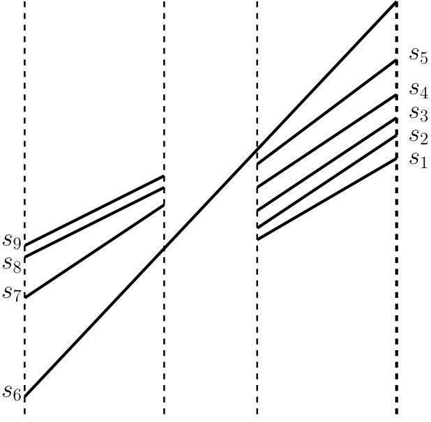 Figure 1
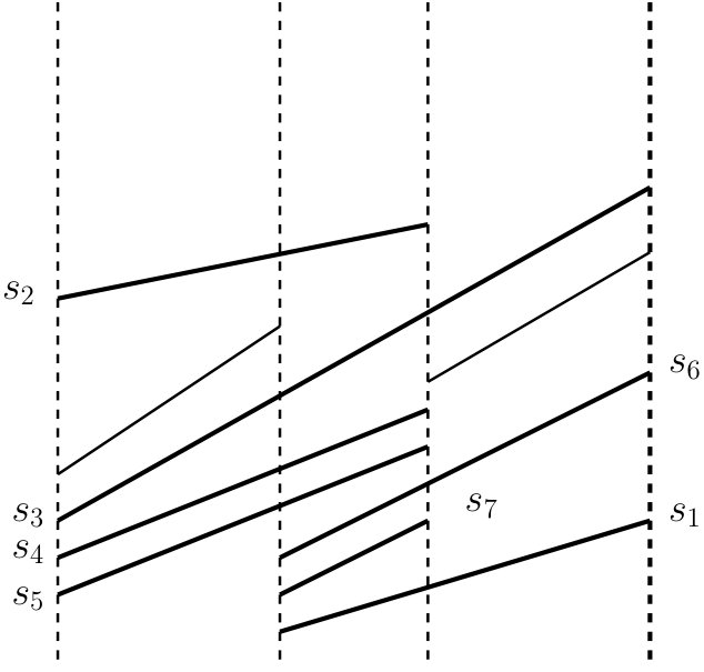 Figure 2
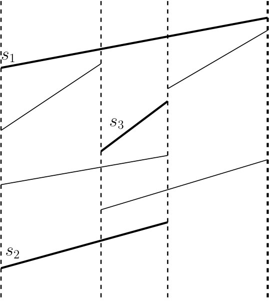 Figure 3
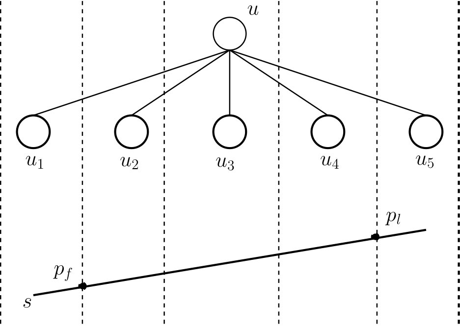 Figure 4
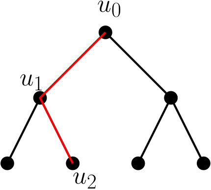 Figure 5
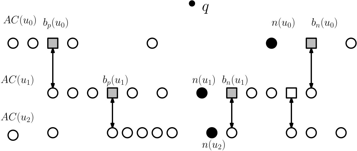 Figure 6
Peer Reviews
No public reviews on file for this paper yet. If you reviewed it on a platform where reviews are public (OpenReview, ICLR, NeurIPS, ICML), you can paste yours below so the community can read it here.
Videos
No videos yet. Explain this paper in a talk, walkthrough, or lecture? Add one.
Taxonomy
TopicsComputational Geometry and Mesh Generation · Algorithms and Data Compression · Machine Learning and Algorithms
Dynamic Planar Point Location in External Memory
J. Ian Munro Cheriton School of Computer Science, University of Waterloo. Email [email protected].
Yakov Nekrich Cheriton School of Computer Science, University of Waterloo. Email: [email protected].
Abstract
In this paper we describe a fully-dynamic data structure for the planar point location problem in the external memory model. Our data structure supports queries in I/Os and updates in amortized I/Os, where is the number of segments in the subdivision and is the block size. This is the first dynamic data structure with almost-optimal query cost. For comparison all previously known results for this problem require I/Os to answer queries. Our result almost matches the best known upper bound in the internal-memory model.
1 Introduction
Planar point location is a classical computational geometry problem with a number of important applications. In this problem we keep a polygonal subdivision of the two-dimensional plane in a data structure; for an arbitrary query point , we must be able to find the face of that contains . In this paper we study the dynamic version of this problem in the external memory model. We show that a planar subdivision can be maintained under insertions and deletions of edges, so that the cost of queries and updates is close to , where is the number of segments in the subdivision and is the block size.
Planar point location problem was studied extensively in different computational models. Dynamic internal-memory data structures for general subdivisions were described by Bentley [11], Cheng and Janardan [16], Baumgarten et al. [9], Arge et al. [3], and Chan and Nekrich [13]. Table 1 lists previous results. We did not include in this table many other results for special cases of the point location problem, such as the data structures for monotone, convex, and orthogonal subdivisions, e.g., [26, 27, 18, 17, 21, 20, 14]. The currently best data structure [13] achieves111In this paper denotes the binary logarithm of when the logarithm base is not specified. query time and update time or query time and update time; the best query-update trade-off described in [13] is randomized query time and update time. See Table 1.
In the external memory model [2] the data can be stored in the internal memory of size or on the external disk. Arithmetic operations can be performed only on data in the internal memory. Every input/output operation (I/O) either reads a block of contiguous words from the disk into the internal memory or writes words from the internal memory into disk. Measures of efficiency in this model are the number of I/Os needed to solve a problem and the amount of used disk space.
Goodrich et al. [22] presented a linear-space static external data structure for point location in a monotone subdivision with query cost. Arge et al. [5] designed a data structure for a general subdivison with the same query cost. Data structures for answering a batch of point location queries were considered in [22] and [8]. Only three external-memory results are known for the dynamic case. The data structure of Agarwal, Arge, Brodal, and Vitter [1] supports queries on monotone subdivisions in I/Os and updates in I/Os amortized. Arge and Vahrenhold [7] considered the case of general subdivisons; they retain the same cost for queries and insertions as [1] and reduce the deletion cost to . Arge, Brodal, and Rao [4] reduced the insertion cost to . Thus all previous dynamic data structures did not break query cost barrier. For comparison the first internal-memory data structure with query time close to logarithmic was presented by Baumgarten et al [9] in 1994. See Table 2. All previous data structures use words of space (or blocks of words222Space usage of external-memory data structures is frequently measured in disk blocks of words. In this paper we measure the space usage in words. But the space usage of words is equivalent to blocks of space.).
In this paper we show that it is possible to break the barrier for the dynamic point location problem. Our data structure answers queries in I/Os, supports updates in I/Os amortized, and uses linear space. Thus we achieve close to logarithmic query cost and a query-update trade-off almost matching the state-of-the-art upper bounds in the internal memory model. Our result is within double-logarithmic factors from optimal. Additionally we describe a data structure that supports point location queries in an orthogonal subdivision with query cost and amortized update cost. The computational model used in this paper is the standard external memory model [2].
2 Overview
2.1 Overall Structure
As in the previous works, we concentrate on answering vertical ray shooting queries. The successor segment of a point in a set of non-intersecting segments is the first segment that is hit by a ray emanating from in the -direction. Symmetrically, the predecessor segment of in is the first segment hit by a ray emanating from in the direction. A vertical ray shooting query for a point on a set of segments asks for the successor segment of in . If we know the successor segment or the predecessor segment of among all segments of a subdivision , then we can answer a point location query on (i.e., identify the face of containing ) in I/Os [7]. In the rest of this paper we will show how to answer vertical ray shooting queries on a dynamic set of non-intersecting segments.
Our base data structure is a variant of the segment tree. Let be a set of segments. We store a tree on -coordinates of segment endpoints. Every leaf contains segment endpoints and every internal node has children for . Thus the height of is . We associate a vertical slab with every node of . The slab of the root node is , where and denote the -coordinates of the leftmost and the rightmost segment endpoints. The slab of an internal node is divided into slabs that correspond to the children of . A segment spans the slab of a node (or simply spans ) if it crosses its vertical boundaries.
A segment is assigned to an internal node , if spans at least one child of but does not span . We assign to a leaf node if at least one endpoint of is stored in . All segments assigned to a node are trimmed to slab boundaries of children and stored in a multi-slab data structure : Suppose that a segment is assigned to and it spans the children , , of . Then we store the segment in , where is the point where intersect the left slab boundary of and is the point where intersects the right boundary of . See Fig. 1. Each segment is assigned to nodes of .
In order to answer a vertical ray shooting query for a point , we identify the leaf such that the slab of contains . Then we visit all nodes on the path from the root of to and answer vertical ray shooting queries in multi-slab structures .
2.2 Our Approach
Thus our goal is to answer ray shooting queries in multi-slab structures along a path in the segment tree with as few I/Os as possible. Segments stored in a multi-slab are not comparable in the general case; see Fig. 2. It is possible to impose a total order on all segments in the following sense: let be a vertical line that intersects segments and ; if the intersection of with is above the intersection of with , then . We can find such a total order in I/Os, where is the number of segments [8, Lemma 3]. But this ordering is not stable under updates: even a single deletion and a single insertion can lead to significant changes in the order of segments. See Fig. 2. Therefore it is hard to apply standard techniques, such as fractional cascading [15, 25], in order to speed-up ray shooting queries. Previous external-memory solutions in [1, 4] essentially perform independent searches in the nodes of a segment tree or an interval tree in order to answer a query. Each search takes I/Os, hence the total query cost is .
Internal memory data structures achieve query cost using dynamic fractional cascading [15, 25]. Essentially the difference with external memory is as follows: since we aim for query cost in internal memory, we can afford to use base tree with small node degree. In this special case the segments stored in sets , , can be ordered resp. divided into a small number of ordered sets. When the order of segments in is known, we can apply the fractional cascading technique [15, 25] to speed up queries. Unfortunately dynamic fractional cascading does not work in the case when the total order of segments in is not known. Hence we cannot use previous internal memory solutions of the point location problem [16, 9, 3, 13] to decrease the query cost in external memory.
In this paper we propose a different approach. Searching in a multi-slab structure is based on a weighted search among segments of . Weights of segments are chosen in such way that the total cost of searching in all multi-slab structures along a path is logarithmic. We also use fractional cascading, but this technique plays an auxiliary role: we apply fractional cascading to compute the weights of segments and to navigate between the tree nodes. Interestingly, fractional cascading is usually combined with the union-split-find data structure, which is not used in our construction.
This paper is structured as follows. In Section 3 we show how our new technique, that will be henceforth called weighted telescoping search, can be used to solve the static vertical ray shooting problem. Next we turn to the dynamic case. In our exposition we assume, for simplicity, that the set of segment -coordinates is fixed, i.e., the tree does not change. We also assume that the block size is sufficiently large, . We show how our static data structure from Section 3 can be modified to support insertions in Section 4. To maintain the order of segments in a multi-slab under insertions we pursue the following strategy: when a new segment is inserted into the multi-slab structure , we split it into a number of unit segments, such that every unit segment spans exactly one child of . Unit segments can be inserted into a multi-slab so that the order of other segments is not affected. The number of unit segments per inserted segment can be large; however we can use buffering to reduce the cost of updates.333As a side remark, this approach works with weighted telescoping search, but it would not work with the standard fractional cascading used in internal-memory solutions [16, 9, 3, 13]. The latter technique relies on a union-split-find data structure (USF) and it is not known how to combine buffering with USF. We need to make some further changes in our data structure in order to support deletions; the fully-dynamic solution for large is described in Section 5. The main result of Section 5, summed up in Lemma 2, is the data structure that answers queries in I/Os; insertions and deletions are supported in and amortized I/Os respectively. We show how to reduce the cost of insertions and the space usage in Sections 6 and Appendix A respectively. We address some missing technical details and consider the case of small block size in Section 7. The special case of vertical ray shooting among horizontal segments is studied in Appendix B. Appendix C provides an alternative introduction to the weighted telescoping search by explaining how this technique works in a simplified scenario. This section is not used in the rest of the paper; the sole purpose of Appendix C is to provide an additional explanation for the weighted telescoping search.
3 Ray Shooting: Static Structure
In this section we show how the weighted telescoping search can be used to solve the static point location problem. Let be the tree, defined in Section 2.1, with node degree for . Let be the set of segments that span at least one child of but do not span .
Augmented Catalogs. We keep augmented catalogs in every node . Each is divided into subsets for ; contains segments that span children , , of and only those children. Augmented catalogs satisfy the following properties:
- (i)
If a segment , then for an ancestor of and spans .
- (ii)
Let for a child of . For any and , , there are at most elements of between any two consecutive elements of .
- (iii)
If , then .
Elements of for some will be called down-bridges; elements of the set , where denotes the parent node of , are called up-bridges. We will say that a sub-list of a catalog bounded by two up-bridges is a portion of . We refer to e.g., [3] or [13] for an explanation how we can construct and maintain . We assume in this section that all segments in every catalog are ordered. We can easily order a set or any set of segments that cross the same vertical line : the order of segments is determined by (-coordinates of) intersection points of segments and . Therefore we will speak of e.g., the largest/smallest segments in such a set.
Element weights. We assign the weight to each element of in a bottom-to-top manner: All segments in a set for every leaf node are assigned weight . Consider a segment , i.e., a segment that spans children , , of some internal node . For let denote the largest bridge in that is (strictly) smaller than and let denote the smallest bridge in that is (strictly) larger than ; we let , where the sum is over all segments and . See Fig. 3 for an example. We set . We keep a weighted search tree for every portion of the list By a slight misuse of notation this tree will also be denoted by . Thus every catalog is stored in a forest of weighted trees where every tree corresponds to a portion of 444In most cases we will omit the subindex and will speak of a weighted tree because it will be clear from the context what portion of is used.. We also store a data structure supporting finger searches on .
Weighted Trees. Each weighted search tree is implemented as a biased -tree with parameters and [10, 19]. The depth of a leaf in a biased -tree is bounded by , where is the weight of an element in the leaf and is the total weight of all elements in the tree. Every internal node has children and every leaf holds segments555In the standard biased ()-tree [10, 19], every leaf holds one element. But we can modify it so that every leaf holds different elements (segments). The weight of a leaf is the total weight of all segments stored in .. In each internal node we keep segments . For every child of and for all and , , is the highest segment from in the subtree of ; if there are no segments from in the subtree of , then . Using values of we can find, for any node of the biased search tree, the child of that holds the successor segment of the query point . Hence we can find the smallest segment in a portion that is above a query point in I/Os where is the total weight of all segments in and is the weight of .
Additional Structures. When the segment is known, we will need to find the bridges that are closest to in order to continue the search. We keep a list for each node and for every , . contains all segments of and some additional segments chosen as follows: is divided into groups so that each group consists of consecutive segments; the only exception is the last group in that contains segments (here we use the fact that segments in are ordered). We choose the constant in such way that every group but the last one contains segments. If a group contains a segment that spans , then we select the highest segment from that spans and the lowest segment from that spans ; we store both segments in . See Fig. 4. For every segment in we also store a pointer to its group in . We keep in a B-tree that supports finger search queries.
Suppose that we know the successor segment of a query point in . We can find the successor segment of in using : Let denote the group that contains . We search in for the segment using finger search. If is not in , we consider the highest segment that spans . By definition of , there are at most segments between and . We can find in I/Os by finger search on using as the finger. Using a similar procedure, we can find the highest bridge segment in .
Queries. A vertical ray shooting query for a point is answered as follows. Let denote the leaf such that the slab of contains . We visit all nodes , , , on the root-to-leaf path where is the root node and . We find the segment in every visited node, where is the successor segment of in . Suppose that is the -th child of ; spans the -th child of . First we search for in the weighted tree of . Next, using the list , we identify the smallest bridge such that and the largest bridge segment such that . The index is chosen so that is the -th child of . We execute the same operations in nodes , , . When we are in a node we consider the portion between bridges and ; we search in the weighted tree of for the successor segment of . Then we identify the lowest bridge and the highest bridge . When all are computed, we find the lowest segment among . Since , is the successor segment of a query point .
The cost of a ray shooting query can be estimated as follows. Let denote the weight of . Let denote the total weight of all segments of (we assume that ). Search for in the weighted tree takes I/Os. By definition of weights, . Hence
[TABLE]
We have and we will show below that . Since , and . Hence the sum above can be bounded by . When is known, we can find and in I/Os, as described above. Hence the total cost of answering a query is . Since every segment is stored in lists , the total space usage is .
It remains to prove that . We will show by induction that the total weight of all elements on every level of is bounded by : Every element in a leaf node has weight ; hence their total weight does not exceed . Suppose that, for some , the total weight of all elements on level does not exceed . Consider an arbitrary node on level , let , , be the children of , and let denote the total weight of elements in . Every element in contributes fraction of its weight to at most different elements in . Hence and the total weight of all elements in does not exceed . Hence, for any level , the total weight of for all nodes on level does not exceed . Hence the total weight of for the root node is also bounded by .
Lemma 1
There exists an -space static data structure that supports point location queries on non-intersecting segments in I/Os.
The result of Lemma 1 is not new. However we will show below that the data structure described in this section can be dynamized.
4 Semi-Dynamic Ray Shooting for : Main Idea
Now we turn to the dynamic problem. In Sections 4 and 5 we will assume666Probably a smaller power of can be used, but we consider to simplify the analysis. that . Overview. The main challenge in dynamizing the static data structure from Section 3 is the order of segments. Deletions and insertions of segments can lead to significant changes in the segment order, as explained in Section 2. However segment insertions within a slab are easy to handle in one special case. We will say that a segment is a unit segment if for some . In other words a unit segment spans exactly one child of . Let denote the conceptual list of all segments that span . When a unit segment is inserted, we find the segments and that precede and follow in ; we insert at an arbitrary position in so that . It is easy to see that the correct order of segments is maintained: the correct order is maintained for the segments that span and other segments are not affected.
An arbitrary segment that is to be inserted into can be represented as unit segments. See Fig. 5 for an example. However we cannot afford to spend operations for an insertion. To solve this problem, we use bufferization: when a segment is inserted, we split it into unit segments and insert them into a buffer . A complete description of the update procedure is given below.
Buffered Insertions. We distinguish between two categories of segments, old segments and new segments. We know the total order in the set of old segments in the portion (and in the list ). New segments are represented as a union of up to unit segments. When the number of new segments in a portion exceeds the threshold that will be specified below, we re-build : we compute the order of old and new segments and declare all segments in to be old.
As explained in Section 3 every portion of is stored in a biased search tree data structure. Each node of has a buffer that can store up to segments. When a new segment is inserted into , we split it into unit segments and add them to the insertion buffer of , where is the root node of . When the buffer of an internal node is full, we flush it, i.e., we move all segments from to buffers in the children of . We keep values , defined in Section 3, for all internal nodes . All and all segments in fit into one block of memory; hence we can flush the buffer of an internal node in I/Os. When the buffer of an internal node is flushed, we do not change the shape of the tree. When the buffer of a leaf node is full, we insert segments from into the set of segments stored in . If necessary we create a new leaf and update the weights of and . We can update the biased search tree in time. We also update data structures for , , . Since a leaf node contains the segments from at most two different groups, we can update all in I/Os. The biased tree is updated in I/Os. The total amortized cost of a segment insertion into a portion is because .
When the number of new segments in is equal to , where is the number of old segments in , we rebuild . Using the method from [8], we order all segments in and update the biased tree. Sorting of segments takes I/Os. We can re-build the weighted tree in I/Os by computing the weights of leaves and inserting the leaves into the new tree one-by-one.
When a new segment is inserted, we identify all nodes where must be stored. For every corresponding list , we find the portion where must be stored. This takes I/Os in total. Then we insert the trimmed segment into each portion as described above. The total insertion cost is . Queries are supported in the same way as in the static data structure described in Section 3. The only difference is that biased tree nodes have associated buffers. Many technical aspects are not addressed in this section. We fill in the missing details and provide the description of the data structure that also supports deletions in Section 5.
5 Ray Shooting for : Fully-Dynamic Structure
Now we give a complete description of the fully-dynamic data structure for vertical ray shooting queries. Deletions are also implemented using bufferization: deleted segments are inserted into deletion buffers that are kept in the nodes of trees . Deletion buffers are processed similarly to the insertion buffers. There are, however, a number of details that were not addressed in the previous section. When a new bridge is inserted we need to change weights for a number of segments. When the segment is found, we need to find the bridges and . The complete solution that addresses all these issues is more involved. First, we apply weighted search only to segments from . We complete the search and find the successor segment in using some auxiliary sets stored in the nodes of . Second, we use a special data structure to find the bridges and . We start by describing the changed structure of weighted trees .
Segments stored in the leaves of are divided into weighted and unweighted segments. Weighted segments are segments from , i.e., weighted segments are used as down-bridges. All other segments are unweighted. Every leaf contains weighted segments. There are at and unweighted segments between any two weighted segments. Hence the total number of segments in a leaf is between and . Only weighted segments in a leaf have non-zero weights. Weights of weighted segments are computed in the same way as explained in Section 3. Hence the weight of a leaf is the total weight of all weighted segments in . The search for a successor of in is organized in such way that it ends in the leaf holding the successor of in . Then we can find the successor of in using auxiliary data stored in the nodes of .
We keep the following auxiliary sets and buffers in nodes of every weighted tree . Let denote the set of segments from that are stored in leaf descendants of a node .
- (i)
Sets and for all such that and for all nodes . () contains highest (lowest) segments from . For every segment in sets and we record the index such that (or NULL if is not a bridge segment).
- (ii)
The set for an internal node is the union of all sets and for all children of .
- (iii)
The set , contains highest segments from that are not stored in any set for an ancestor of . Either holds at least and at most segments or holds less than segments and for all descendants of are empty. In other words, are organized as external priority search trees [6]. The set is defined in the same way with respect to the lowest segments. We use and to maintain sets and .
- (iv)
Finally we keep an insertion buffer and a deletion buffer in every node .
Deletions. If an old segment is deleted, we insert it into the deletion buffer of the root node . If a new segment is deleted, we split into unit segments and insert them into . When one or more segments are inserted into , we also update sets and . For any node , when the number of segments in exceeds , we flush both and using the following procedure. First we identify segments and remove such from both and . Next we move segments from and to buffers and in the children of . For every child of , first we update sets by removing segments from (resp. inserting segments from ) if necessary. Then we take care that the size of is not too small. If some contains less than segments and more than [math] segments, we move up segments from the children of into , so that the total size of becomes equal to or all segments are moved from the corresponding sets in the children of into . We recursively update in each child of using the same procedure.
Next, we update sets . We compute where the union is taken over all proper ancestors of . Every segment in is either from or from for a proper ancestor of . Hence we can compute all when and are known. Sets and are updated in the same way. Finally we update the set by collecting segments from and .
All segments needed to re-compute sets after flushing buffers and fit into one block of space. Hence we can compute the set in I/Os and all sets in each node in I/Os. The set is updated in I/Os. Since each node has children, the total number of I/Os needed to flush a buffer is . Every segment can be divided into up to unit segments and each unit segment can contribute to buffer flushes. Hence the total amortized cost per segment is . We did not yet take into account the cost of refilling the buffers ; using the analysis similar to the analysis in [12, Section 4], we can estimate the cost of re-filling as .
We do not store buffers in the leaf nodes. Let be the set of segments kept in a leaf and let be the set of weighted segments stored in . When we move segments from or to its leaf child , we update accordingly. This operation changes the weight of . Hence we need to update the weighted tree in I/Os. Sets and are also updated.
After an insertion of new segments into a leaf node, we may have to insert or remove some bridges in for . When we insert a new bridge into , we must split some portion into two new portions, and . Additionally we must change the weights of the bridge segments in that precede and follow . The cost of splitting is . We also need I/Os to change the weights of two neighbor bridges. Hence the total cost of inserting a new bridge is . We insert a bridge at most once per insertions into because every new segment is divided into up to unit segments. We remove a bridge at most once after deletions. See [13] for the description of the method to maintain bridges in catalogs . Thus the total amortized cost incurred by a bridge insertion or deletion is .
Insertions. Insertions are executed in a similar way. A new inserted segment is split into unit segments that are inserted into the buffer for the root node . The buffers and auxiliary sets are updated and flushed in the same way as in the case of deletions. When the number of new segments in some portion is equal to , where is the number of old segments in , we rebuild . As explained in Section 4, rebuilding of incurs an amortized cost of .
Queries. The search for the successor segment in the weighted tree consists of two stages. Suppose that the query point is in the slab of the -th child of . First we find the successor of in by searching in . We traverse the path from the root to the leaf holding . In every node we select its leftmost child , such that for some contains a segment that is above and is not deleted (i.e., for all ancestors of ). The size of each set is larger than the total size of all in all ancestors of . Hence every contains some elements that are not deleted unless the set is empty. Therefore we select the correct child in every node. Since is a biased search tree [10, 19], the total cost of finding the leaf is bounded by where is the total weight of all segments in and is the weight of the bridge segment .
During the second stage we need to find the successor segment of in . The distance between and in can be arbitrarily large. Nevertheless is stored in one of the sets for some ancestor of . Suppose that is an unweighted segment stored in a leaf of and let denote the lowest common ancestor of and . Let be the child of that is an ancestor of . There are at most segments in between and . Hence, is stored in the set . Hence, is also stored in . We visit all ancestors of and compute . Then we visit all ancestors one more time and find the successor of in . The asymptotic query cost remains the same because we only visit the nodes between and the root and each node is visited a constant number of times.
We need to consider one additional special case. It is possible that there are no bridge segments stored in the leaves of . In this case there are at most segments in for every pair , satisfying , stored in the leaves of . For each portion , if there are at most segments in , we keep the list of all such segments. All such lists fit into one block of memory. We also keep the list of indexes , such that is empty.Suppose that we need to find the successor of and is empty. Then we simply examine all segments in for all and find the successor of in I/Os.
When is known, we need to find and , if was not computed at the previous step. It is not always possible to find these bridges using because and can be outside of . To this end, we use the data structure for colored union-split-find problem on a list (list-CUSF) that will be described in Section B.1. We keep the list containing all down-bridges from , for , and all up-bridges from . Each segment in is associated to an interval; a segment is associated to an interval and a segment from is associated to a dummy interval . For any segment we can find the preceding/following segment associated to an interval for any , , in I/Os. Updates of are supported in I/Os. Since we insert or remove bridge segments once per updates, the amortized cost of maintaining the list-CUSF structure is .
Summing up. By the same argument as in Section 3, weighted searches in all nodes take I/Os in total. Additionally we spend I/Os in every node with a query to list-CUSF. Thus the total query cost is . When a segment is deleted, we remove it from lists and from secondary structures (weighted trees etc.) in these nodes. The deletions take I/Os per node or I/Os in total. When a segment is inserted, it must be inserted into lists . We first have to spend I/Os to find the portion of each where it must be stored. When is known, an insertion takes amortized I/Os as described above. The total cost of an insertion is I/Os. Since every segment is stored in lists, the total space is .
Lemma 2
If , then there exists an space data structure that supports vertical ray shooting queries on a dynamic set of non-intersecting segments in I/Os. Insertions and deletions of segments are supported in and amortized I/Os respectively.
6 Faster Insertions
When a new segment is inserted into our data structure, we need to find the position of in lists (to be precise, we need to know the portion of that contains ). When positions of in are known, we can finish the insertion in I/Os. In order to speed-up insertions, we use the multi-colored segment tree of Chan and Nekrich [13]. Segments in lists are assigned colors , so that the total number of different colors is where is the height of the segment tree. Let denote the set of segments of color in . We apply the technique of Sections 3- 5 to each color separately. That is, we create augmented lists and construct weighted search trees for each color separately. The query cost is increased by factor , the number of colors. The deletion cost is also increased by factor because we update the data structure for each color separately. When a new segment is inserted, we insert it into some lists where is the node such that spans but does not span its parent and is some color (the same segment can be assigned different colors in different nodes ). We can find the position of in all with I/Os where is the query cost in a union-split-find data structure in the external memory model. See [13] for a detailed description.
Lemma 3
If , then there exists an space data structure that supports vertical ray shooting queries on a dynamic set of non-intersecting segments in I/Os. Insertions and deletions of segments can be supported in amortized I/Os.
7 Missing Details
Using the method from [13] we can reduce the space usage of our data structure to linear at the cost of increasing the query and update complexity by factor.The resulting data structure supports queries in I/Os and updates in amortized I/Os. See Section A for a more detailed description.
In our exposition we assumed for simplicity that the tree does not change, i.e., the set of -coordinates of segment endpoints is fixed and known in advance. To support insertions of new -coordinate, we can replace the static tree with a weight-balanced tree with node degree . We also assumed that the block size is large, . If , the linear-space internal memory data structure [13] achieves query cost and update cost because and for . Thus we obtain our main result.
Theorem 1
There exists an space data structure that supports vertical ray shooting queries on a dynamic set of non-intersecting segments in I/Os. Insertions and deletions of segments are supported in amortized I/Os.
Appendix A Saving Space
We use another method from [13] to reduce the space usage of the data structure in Lemma 3 to linear.
Lemma 4** ([13], Lemma 3.1)**
Consider a decomposable search problem, where (i) there is an -space fully dynamic data structure with query cost and update cost, and (ii) there is an -space deletion-only data structure with query cost, update cost, and preprocessing cost. Then there is an -space fully dynamic data structure with query cost and amortized update cost for any given parameter (assuming that is nondecreasing).
Lemma 5** ([13], Lemma 3.1)**
If there is a deletion-only data structure for vertical ray shooting queries for horizontal segments with space, query cost, update cost, and preprocessing cost, then there is a deletion-only data structure for vertical ray shooting queries for arbitrary non-intersecting segments with space, query cost, update cost, and preprocessing cost.
The two above lemmata are obtained by a straightforward extension of Lemmata 3.1 and 3.2 from [13] to the external memory model. We will describe in Section B.3 a data structure that supports vertical ray shooting queries on a set of horizontal segments in I/Os and updates within the same amortized bounds. If we plug this result into Lemma 5, we obtain a deletion-only data structure for ray shooting queries in a set of arbitrary non-intersecting segments with query cost, deletion cost, and preprocessing cost. Recall that the structure of Lemma 3 has query cost , update cost I/Os amortized, and space usage . We apply Lemma 4 to the structure of Lemma 3 and the deletion-only structure described above. We obtain the following lemma.
Lemma 6
If , then there exists an space data structure that supports vertical ray shooting queries on a dynamic set of non-intersecting segments in I/Os. Insertions and deletions of segments are supported in amortized I/Os.
Appendix B Ray Shooting on Horizontal Segments
In this section we describe a data structure for vertical ray shooting queries in a dynamic set of horizontal segments. A data structure for this problem can be used to answer dynamic point location queries in an orthogonal subdivision. The special case of horizontal segments is much simpler than the ray shooting among arbitrary segments because it is easy to maintain the order among horizontal segments. Our solution is based on a colored variant of the predecessor search, described in Section B.1. We describe how this data structure can be combined with the segment tree to answer ray shooting queries in Section B.2. We show that the space usage of our data structure can be reduced from to in Section B.3.
B.1 Colored Predecessor Search in External Memory
In the colored predecessor searching problem, every element has a value and color interval , . We assume that color intervals are disjoint for elements with the same value, i.e., if for two elements and , then . The answer to a colored predecessor query for and is the largest (with respect to its value ) element , such that and . We say than an element is colored with a color if . First, we show how colored search queries for a small set of elements can be answered with a constant number of I/Os. Then, we will describe a data structure for an arbitrarily large set of elements.
Lemma 7
Let and . The colored predecessor searching problem for a set , such that colors of elements belong to for , can be solved in I/Os using a space data structure that supports updates in I/Os.
- Proof: We sort the elements in by their values (elements with the same value are sorted by the smallest colors that belong to their color intervals) and store them in the leaves of a tree . Each leaf contains elements of and each internal node has children. We say that an internal node contains an element if is stored in a leaf descendant of . In every internal node , we store a table : for each and each , iff the -th child of contains at least one element with color . For every such that , we also store the maximal and the minimal elements colored with that belong to the -th child of . Every table fits into blocks. There are internal nodes in ; hence, all use words of space.
The search for starts at the root of . In each visited node of , we identify the rightmost child such that for some and the minimal element colored with in is not greater than . If such does not exist, then contains no element colored with that is smaller than or equal to . Otherwise, the search continues in . The height of is and the search takes I/Os.
When a new element is inserted into , we insert it into a leaf of . Then, we visit all ancestors of and update the tables . The tree can be rebalanced in a standard way. Deletions are processed with a symmetric procedure.
Lemma 8
Let . A colored searching problem for a set of elements, such that values of elements belong to the universe and colors belong to the interval for , can be solved in I/Os using a space data structure that supports updates in amortized I/Os.
- Proof: To simplify the description, we introduce a new set of interval colors : for each interval , , there is an interval color . Thus each interval color corresponds to a color interval . Obviously, for each original color there is the interval color that corresponds to the interval . An element is colored with a color from a set if and only if is colored with an interval color from a set . For every set of colors the equivalent set of interval colors can be constructed in I/Os. While each element is colored with colors from an interval , each is colored with only one interval color.
The data structure can be defined recursively. If , we can use the data structure of Lemma 7 and answer queries in I/Os. If , then we divide the interval into subintervals of size777For ease of description we assume that is an integer. for . The array contains two tables and for each subinterval. The table ( contains the minimal (maximal) element in the -th subinterval colored with an interval color . If there is no such element in the -th subinterval, then . Let be the set of elements whose values belong to the subinterval and whose interval color is . If , the values of elements from are already stored in and . If for at least one pair , we construct a recursively defined data structure for . All values of elements in are specified relative to the left end of the -th subinterval; thus values of all elements in belong to . The data structure supports colored predecessor searching in the array : if , then contains an element with and , i.e. is colored with an interval color . Values of elements in also belong to the interval . All tables and in the array have entries. Therefore uses words of space. Since values of elements in and belong to , there are at most recursion levels. Hence, the total space usage is .
A query is processed as follows. Let be the set of interval colors that is equivalent to . If , the query is answered in I/Os by Lemma 7. Otherwise we check whether there is at least one pair such that and ; here denotes the index of the subinterval that contains . This condition can be tested in I/Os because each entry of fits into one block of memory. If such a pair exists, the search continues in the data structure . Otherwise, we use the data structure to find the largest such that is colored with a color . The answer to the query is the maximal element among all such that .
Suppose that and an element is inserted. We update the values of and for if necessary. If after the insertion of , we insert an element , such that and into . If after the insertion of , we insert an element into the data structure . Deletions are symmetric to insertions.
In the colored union-split-find (CUSF) problem we put an additional restriction on queries: only queries , such that there is an element with value , are allowed. Moreover, we assume that a pointer to such an element is provided with a query. When an element is deleted or inserted, we assume that the position of is known.
Lemma 9
The CUSF problem for a set of elements and , , colors can be solved in I/Os using a space data structure that supports updates in amortized I/Os.
- Proof: We can transform the general searching data structure into a CUSF data structure using the same principle as in [20]. The set of elements is divided into chunks of size . If , then we set . Otherwise, we set . We assign to each chunk an ordered label : if the chunk follows , then . Labels can be maintained according to the algorithm of [24, 28]: when a new chunk is inserted or when a chunk is deleted, labels must be changed. The set of interval colors is defined exactly as in the proof of Lemma 8. The data structure contains an element if and only if the chunk contains an element with color interval . By Lemma 8, uses words of space. We also store a data structure for each chunk that supports colored predecessor searching queries in this chunk. We implement the data structure as described in Lemma 7, so that colored searching queries are supported in I/Os. All data structures use space .
Consider a query . Suppose that some element with belongs to a chunk . First, we find the largest chunk , such that contains at least one interval color and . The set of colors can be constructed with I/Os. Using , we can answer the colored search query for and find the chunk in I/Os. The largest element with and belongs to the chunk . The cost of finding using the data structure for the chunk is ; hence, a query can be answered with I/Os.
When a new element is inserted, we insert it into a chunk in I/Os. If the data structure does not contain the element , then we insert this element into in I/Os. If the number of elements in a block equals we distribute the elements of between two chunks and . It takes I/Os to delete the data structure and insert the elements of into data structures and . We assign new labels to chunks and and update the set of labels. This leads to changing the labels of chunks. The data structure contains labels for each chunk. Hence, the total number of updates in incurred by updating the set of labels is . If , then . If , then . Since labels are changed after insertions, the amortized cost of an insertion is . Deletions are performed in the same way. Thus the total cost of an update is .
We remark that, in fact, the values of elements are not necessary. Using the same method, we can store a list of elements, such that each element in the list is assigned an interval of colors . Given a pointer to a list element and a color interval , we ask for the first element that follows in the list and . We will call this problem list CUSF.
Lemma 10
The list CUSF problem for a set of elements and , , colors can be solved in I/Os using a space data structure that supports updates in amortized I/Os.
This result can be proved in the same way as Lemma 9; we use it in Section 5.
B.2 Ray Shooting on Horizontal Segments
Structure. All segments are stored in a tree with node degree for some constant . The leaves of contain -coordinates of segment endpoints; every leaf contains elements. The tree is organized as a variant of the segment tree, in the same way as in Section 2.1. We start by introducing some additional notation. The range of a leaf node is the interval , where and are the minimal and the maximal values stored in . The range of an internal node is the interval , so that and are the minimal and maximal values stored in leaf descendants of .
We say that a segment covers an interval if and ; a segment covers if it covers an interval . Thus a segment spans a node if it covers the range of . We implement in the same way as before: a segment is associated with a node if and only if spans at least one child of , but does not span the node . Thus each segment is associated with nodes.
Let be the set of segments associated with a node . For simplicity, we sometimes will not distinguish between a segment and its -coordinate. For any point , let denote search path for in the tree . Each segment , , is stored in a list , . If covers and is an internal node, then spans the child of , . Hence, we can identify the predecessor segment of by finding the highest segment , , such that spans some node and .
Our method is based on Lemma 9 and the fractional cascading technique [25] applied to sets . We construct augmented catalogs for all nodes of . For a leaf node , . Every list is divided into groups , so that each group contains between and segments. We guarantee that for an internal node contains one segment from a group for every child of and every group . Moreover, contains all segments from . If copies of the same segment are stored in augmented lists for a node and for a child of , then the two copies of in and are connected by pointers, called bridges. Thus there are elements of between any two consecutive bridges from to .
The data structure contains the colored set of (-coordinates of) all segments in : if a segment spans children of , then an element with value and colors is stored in ; if a segment does not span any child of (i.e., belongs to ), then is colored with a dummy color . The data structure also contains a colored set of segments in , but segments are colored according to a different rule. All segments from are colored with a dummy color ; for any segment , the set of colors for contains all values such that belongs to for a child of . Both and are implemented as described in Lemma 9.
Queries. The search procedure visits all nodes on the path starting at the root. In every internal node , we identify the predecessor of in . Then we identify the highest segment in such that is below and spans the child of , . Finally, we examine all segments in the leaf and find the predecessor segment of stored in . The predecessor segment of in is the highest segment among all for .
We can identify for the root of in I/Os using a standard B-tree. Suppose that for a node is known. We will show how to find and for the child of . The highest segment , such that is below and spans a child of can be found by answering the query to a data structure . The segment can be identified as follows. The highest segment , such that is below and belongs to can be found in I/Os using . Suppose that the copy of belongs to a group in . Since is the highest segment below in , either belongs to the group or to the next group . If we store -coordinates of all segments from each group in a B-tree, then we can search in in I/Os because each contains segments. Thus the segment can be found in I/Os if is known. Since the search procedure spends I/Os in every node of , the total cost of the search is .
Updates. Every segment belongs to lists . Every insertion into a list can be handled as follows. All nodes such that belongs to are situated on at most two root-to-leaf paths . We can identify positions of the -coordinate of in all that belong to some path in I/Os as described in the search procedure.
When we know the position of in a list , we insert into data structures and in I/Os. We also insert into the B-tree for its group in . If the number of elements in exceeds , is split into two groups and . The list for the parent of already contains one element from either or . A representative of another group must be inserted into . The position of in can be found in I/Os; after that, is inserted into in I/Os as described above. It can be shown that an insertion into a catalog leads to insertions into augmented lists of ancestors of [25]. Hence, the total cost of an insertion is . Deletions can be handled in the same way. Since every segment is stored in nodes, the total space usage is .
Lemma 11
There exists a space data structure that supports ray shooting queries on horizontal segments in I/Os and updates in amortized I/Os.
We can reduce the space usage to linear using the same approach as in [9, 20]. For completeness, we provide the proof in Section B.3.
Theorem 2
There exists a space data structure that supports ray shooting queries on horizontal segments in I/Os and updates in amortized I/Os.
B.3 Reducing Space to Linear
We follow the same approach as in [9, 20]. For a segment , let be the lowest common ancestor of the leaves in which and are stored. The node is the lowest node such that the range of contains , but does not span . Suppose that spans the children of . We represent as a union of three segments: , , and , where and . Segments , and are stored in sets , , and respectively. Let , , and . A ray shooting query can be answered by answering a ray shooting query for , , and .
We can identify the predecessor segment of in by storing all segments in the data structure of section B.2. Since every segment is stored only once the total space usage is . Now we describe the data structure for . A query on can be answered using a symmetrically defined data structure.
Each set is divided into blocks , so that each block contains segments. We denote by the segment in a block with the largest -coordinate of the right endpoint. The segments for all blocks and all sets are stored in a data structure implemented as in section B.2. Since the total number of segments in is , needs words. We denote by the set of -coordinates of all segments in . The data structure is defined on all sets . Let denote the nodes that lie on some root-to-leaf path of . Using , we can search in all sets in I/Os per node. To implement , we apply the construction of section B.2, i.e., the augmented sets and CUSF structures, to sets . Finally, for each block we store a data structure that supports queries on segments of in I/Os. This data structure uses the fact that the left endpoints of all segments in lie on the same vertical line and is very similar to an external memory priority search tree [6].
A point location query for on can be answered as follows. We start by identifying the successor segment of in and the predecessor segment of in . Let and denote the coordinates of and . Then, we use the data structure and find and for every node , where is the search path for in . The following fact is proved in [20].
Fact 1
Let and be the blocks in that contain segments with -coordinates and respectively. Let be the predecessor segment of in . Then belongs to a block or for some .
We can complete the search by querying all and , , in I/Os and selecting the highest segment among all answers.
When a new segment is inserted, we identify the node in I/Os. Insertion of into is handled as in section B.2. Insertion of starts with identifying the child of such that intersects with but does not span . Let be the block of into which must be inserted. If the -coordinate of the right endpoint of is larger than the -coordinate of , then we remove from and insert into . We also insert the -coordinate of into . Finally, if the number of elements in after an insertion equals , then is split into two blocks that contain segments each. We can show using standard methods that the amortized cost of splitting a block is . An insertion into is symmetric. Hence, the total cost of an insertion is . Deletions can be implemented in the same way.
Appendix C Weighted Telescoping Search: Simplified Scenario
In this section we provide a simple alternative description of our main technique, the weighted telescoping search. This section is not necessary in order to understand the material in the rest of this paper; the only purpose of this section is to provide a simple description of the weighted telescoping search. To introduce our technique, we digress from the point location problem and consider the following more simple scenario. Suppose that we are given a balanced tree of node degree and we keep a list (or catalog) in every node of . We assume that elements of are numbers. The successor of in a set is the smallest element in that is larger than or equal to , . Suppose that we want to traverse a path from the root of to a leaf and search for the successor of some in the union of all lists along the path. In other words, for any element and any leaf we want to quickly find . This problem can be solved using the standard fractional cascading technique [15] within the same time, but in this paper we describe an alternative solution. We also believe that this general technique can be used in other scenarios when the standard fractional cascading is hard to apply. Unlike the rest of this paper, in this section we describe the solution for the internal memory model.
Our solution is based on assigning weights to elements of and maintaining a forest of weighted trees on each list for every node . Roughly speaking, we choose the weights in such a way that the weight of an element gives us an estimate on the number of elements , such that is stored in for some descendant of and . We keep augmented catalogs in order to compute and maintain element weights.
Augmented Lists. We maintain an augmented catalog in every node . Augmented catalogs are supersets of , , that satisfy the following properties:
- (i)
If , then for an ancestor of .
- (ii)
Let a subset of be defined as for a child of . There are at most elements of between any two consecutive elements of .
Elements of for some will be called down-bridges; elements of the set , where denotes the parent node of , are called up-bridges. We will say that a sub-list of a catalog bounded by two up-bridges is a portion of . We can create and maintain augmented lists using the fractional cascading technique [15, 25]. The main idea is to copy selected elements from and store the copies in lists for descendants of ; see e.g., [13] for a detailed description. If the same element is stored in lists and , where is the parent node of , then we assume that there are pointers between instances of in and .
Element weights. We assign the weight to each element of in a bottom-to-top manner: for a leaf node every element is assigned weight . Consider an internal node with children , , . We associate values with each for every , . Let and denote two consecutive bridge elements in . Let denote the total weight of all elements such that . Every element that satisfies is assigned the same value of
[TABLE]
The weight of is defined888We observe that the same element can be assigned different weights in different nodes . as .
Telescoping Search. Consider a sub-list of the augmented catalog bounded by two up-bridges. All elements of are stored in a weighted search tree satisfying the following property: The depth of a leaf holding an element is bounded by where is the total weight of all elements in . We can use e.g. biased search trees [10, 19] for this purpose.
Now suppose that we want to find, for some number and some leaf of , the successor of in where is the path from the root to . We start in the root node and identify . Suppose that is the -th child of . We find the largest down-bridge and the smallest down-bridge where and . We use finger search [23] in with as a finger to find and in time. Next we identify the portion bounded by and . We find by searching in the weighted tree for . We then find the largest and the smallest where , and is the -th child of . Again we use finger search and find , in time. We continue in the same way until the leaf node is reached. See Fig. 6.
When we know for every node , can be computed. Every element is either from the set or from the set for some ancestor of . Hence . Hence is the successor of in .
The total time can be estimated as follows. Let denote the weight of . We can find the element in time , where is the total weight of all elements in . Down-bridges and can be found in time by finger search in . When we know and , we can compute in time where is the total weight of all elements in . When is known, we can compute and in time. The total time needed to compute all is where is the tree height. Since , we have
[TABLE]
By definition, . We will show below that . Since , and the sum above can be bounded by . All finger searches also take time.
It remains to prove that . We will show by induction that the total weight of all elements on every level of is bounded by : Every element in a leaf node has weight ; hence their total weight does not exceed . Suppose that, for some , the total weight of all elements on level does not exceed . Consider an arbitrary node on level , let , , be the children of , and let denote the total weight of elements in . Every element in contributes fraction of its weight to at most different elements in . Hence and the total weight of all elements in does not exceed . Hence, for any level , the total weight of for all nodes on level does not exceed . Hence the total weight of for the root node is also bounded by .
Thus we have shown the following result.
Lemma 12
Suppose that we store a sorted list in every node of a balanced degree- tree . Then it is possible to find for any and for any root-to-leaf path in time, where is the total size of all lists . The underlying data structure uses space .
It is possible to extend the result of this section to the external memory model and to dynamize our data structure. However Lemma 12 cannot be used to answer vertical ray shooting queries because in the scenario of this Lemma lists contain numbers.
The reference list from the paper itself. Each links out to its DOI / PubMed record.
- 1[1] Pankaj K. Agarwal, Lars Arge, Gerth Stølting Brodal, and Jeffrey Scott Vitter. I/O-efficient dynamic point location in monotone planar subdivisions. In Proc. 10th Annual ACM-SIAM Symposium on Discrete Algorithms, (SODA) , pages 11–20, 1999.
- 2[2] Alok Aggarwal and Jeffrey Scott Vitter. The Input/Output complexity of sorting and related problems. Commun. ACM , 31(9):1116–1127, 1988.
- 3[3] Lars Arge, Gerth Stølting Brodal, and Loukas Georgiadis. Improved dynamic planar point location. In Proceedings of the 47th Annual IEEE Symposium on Foundations of Computer Science , pages 305–314, 2006.
- 4[4] Lars Arge, Gerth Stølting Brodal, and S. Srinivasa Rao. External memory planar point location with logarithmic updates. Algorithmica , 63(1-2):457–475, 2012.
- 5[5] Lars Arge, Andrew Danner, and Sha-Mayn Teh. I/O-efficient point location using persistent B-trees. ACM Journal of Experimental Algorithmics , 8, 2003.
- 6[6] Lars Arge, Vasilis Samoladas, and Jeffrey Scott Vitter. On two-dimensional indexability and optimal range search indexing. In Proc. 18th ACM SIGACT-SIGMOD-SIGART Symposium on Principles of Database Systems (PODS) , pages 346–357, 1999.
- 7[7] Lars Arge and Jan Vahrenhold. I/O-efficient dynamic planar point location. Computational Geometry , 29(2):147–162, 2004.
- 8[8] Lars Arge, Darren Erik Vengroff, and Jeffrey Scott Vitter. External-memory algorithms for processing line segments in geographic information systems. Algorithmica , 47(1):1–25, 2007.