Root Cones and the Resonance Arrangement
Samuel C. Gutekunst, Karola M\'esz\'aros, and T. Kyle Petersen

TL;DR
This paper explores the structure and enumeration of resonance chambers related to root polytopes and hyperplane arrangements, revealing asymptotic growth and connections to polynomiality and threshold functions.
Contribution
It introduces new data structures for labeling resonance chambers and establishes asymptotic estimates for their number, linking geometric, combinatorial, and algebraic perspectives.
Findings
Number of resonance chambers grows asymptotically as 2^{n^2}
Connections established between resonance chambers, Kostant partition function, and threshold functions
New data structures improve understanding of chamber enumeration
Abstract
We study the connection between triangulations of a type root polytope and the resonance arrangement, a hyperplane arrangement that shows up in a surprising number of contexts. Despite an elementary definition for the resonance arrangement, the number of resonance chambers has only been computed up to the dimensional case. We focus on data structures for labeling chambers, such as sign vectors and sets of alternating trees, with an aim at better understanding the structure of the resonance arrangement, and, in particular, enumerating its chambers. Along the way, we make connections with similar (and similarly difficult) enumeration questions. With the root polytope viewpoint, we relate resonance chambers to the chambers of polynomiality of the Kostant partition function. With the hyperplane viewpoint, we clarify the connections between resonance chambers and threshold…
Click any figure to enlarge with its caption.
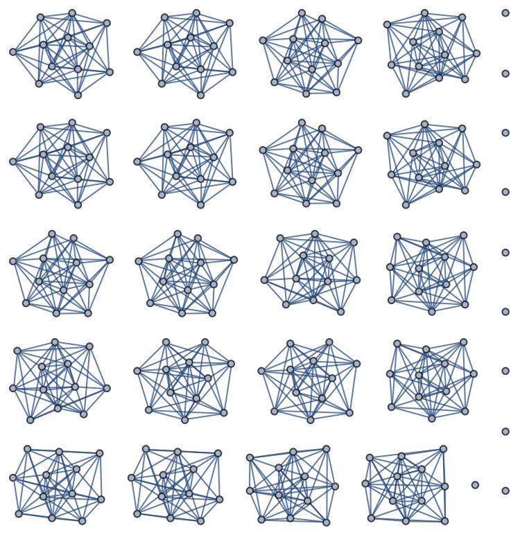 Figure 1
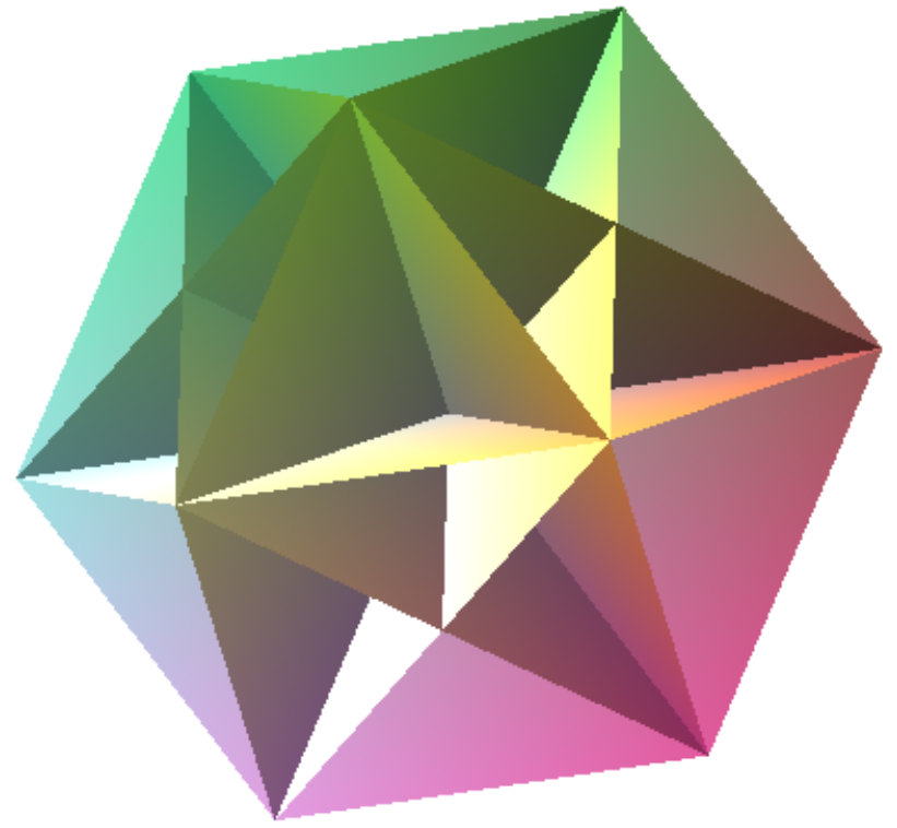 Figure 2
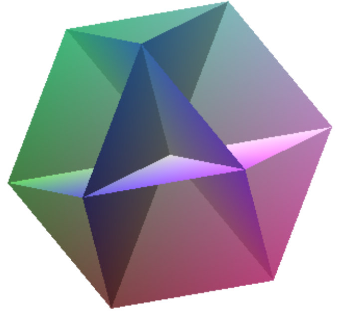 Figure 3
| 1 | 2 | 2 | 2 | 2 | 2 | 2 |
| 2 | 5 | 6 | 7 | 7 | 8 | 16 |
| 3 | 26 | 32 | 48 | 52 | 74 | 512 |
| 4 | 294 | 370 | 820 | 941 | 1882 | 65536 |
| 5 | 8866 | 11292 | 44288 | 47286 | 152292 | 33554432 |
| 6 | 821851 | 1066044 | ? | 7514067 | 43415794 | 68719476736 |
| 7 | 261814714 | 347326352 | ? | 4189035432 | 46574750770 | 562949953421312 |
| 8 | 308698937454 | 419172756930 | ? | 8780769776473 | ? | 18446744073709551616 |
| 1 | 1 | 1 | 1 | 2 |
| 2 | 2.4 | 2.6 | 2.8 | 4.0 |
| 3 | 4.7 | 5 | 5.7 | 6.7 |
| 4 | 8.2 | 8.5 | 9.9 | 10.5 |
| 5 | 13.1 | 13.5 | 15.5 | 15.7 |
| 6 | 19.6 | 20.0 | 22.8 | 22.5 |
| 7 | 28.0 | 28.4 | 32.0 | 31.0 |
| 8 | 38.2 | 38.6 | 43.0 | 41.3 |
Peer Reviews
No public reviews on file for this paper yet. If you reviewed it on a platform where reviews are public (OpenReview, ICLR, NeurIPS, ICML), you can paste yours below so the community can read it here.
Videos
No videos yet. Explain this paper in a talk, walkthrough, or lecture? Add one.
Root cones and the resonance arrangement
Samuel C. Gutekunst
,
Karola Mészáros
and
T. Kyle Petersen
Operations Research and Information Engineering, Cornell University, Ithaca, NY 14853
Department of Mathematics, Cornell University, Ithaca, NY 14853 and School of Mathematics, Institute for Advanced Study, Princeton, NJ 08540
Department of Mathematical Sciences, DePaul University, Chicago, IL 60614
[email protected], [email protected], [email protected]
Abstract.
We study the connection between triangulations of a type root polytope and the resonance arrangement, a hyperplane arrangement that shows up in a surprising number of contexts. Despite an elementary definition for the resonance arrangement, the number of resonance chambers has only been computed up to the dimensional case. We focus on data structures for labeling chambers, such as sign vectors and sets of alternating trees, with an aim at better understanding the structure of the resonance arrangement, and, in particular, enumerating its chambers. Along the way, we make connections with similar (and similarly difficult) enumeration questions. With the root polytope viewpoint, we relate resonance chambers to the chambers of polynomiality of the Kostant partition function. With the hyperplane viewpoint, we clarify the connections between resonance chambers and threshold functions. In particular, we show that the base-2 logarithm of the number of resonance chambers is asymptotically .
Work of Gutekunst supported by the National Science Foundation Graduate Research Fellowship Program under Grant No. DGE-1650441. Work of Mészáros partially supported by a National Science Foundation Grant (DMS 1501059) as well as by a von Neumann Fellowship at the IAS funded by the Fund for Mathematics and the Friends of the Institute for Advanced Study. Work of Petersen supported by a Simons Foundation collaboration travel grant. Any opinions, findings, and conclusions or recommendations expressed in this material are those of the authors and do not necessarily reflect the views of the National Science Foundation.
1. Introduction
This is a story of three counting problems:
- (1)
the number of chambers of polynomiality of the Kostant partition function, 2. (2)
the number of threshold functions, and 3. (3)
the number of maximal unbalanced families.
All three counting problems have resisted exact enumeration beyond small cases. We find in Sloane’s On-Line Encyclopedia of Integer Sequences [35] that problem (1) has 6 entries (A119668), problem (2) has 10 entries (A000609), and problem (3) has 8 entries (A034997). The purpose of this article is to provide some links between these problems and to suggest some data structures that might prove useful for either exact or asymptotic enumeration.
1.1. Kostant chambers
Vector partition functions are fundamental in mathematics. A special vector partition function associated to the type root system is the Kostant partition function, which was introduced by Bertram Kostant in 1958 in order to write down the multiplicity of a weight of an irreducible representation of a semisimple Lie algebra, also known as the Weyl character formula or Kostant multiplicity formula [23, 24]. Kostant partition functions are ubiquitous in mathematics, appearing not only in representation theory, but in algebraic combinatorics, toric geometry and approximation theory, among other areas.
The Kostant partition function is a piecewise polynomial function [36] whose domains of polynomiality are maximal convex cones in the common refinement of all triangulations of the convex hull of the positive roots (see [12]), which we will refer to as Kostant chambers. Let denote this collection of cones, and let denote the number of Kostant chambers. For example, Figure 1 shows the seven chambers of .
The inspiration for our work stems from an open problem posed by Kirillov [22] and its investigation by de Loera and Sturmfels in [12].
Question 1**.**
How many chambers of polynomiality does the Kostant partition function have?
It is an open problem to show that enumerating is #P-hard [11]. The values of have been calculated up to by de Loera and Sturmfels [12]. See Table 1.
1.2. Threshold functions
The study of linear threshold functions has a long history of applications in a variety disciplines, including Economics, Psychology, and Computer Science [30]. These are boolean functions of the form for some threshold and some vector known as the weight vector.
It is well-known that threshold functions correspond to their weight vectors only up to the half-spaces determined by negative/nonnegative dot products with vectors (see, e.g., [38]). That is, threshold functions are in bijection with the chambers in the hyperplane arrangement whose normal vectors are all vectors, representing vertices of an -cube. Let denote this arrangement of hyperplanes, which we call the threshold arrangement, and let denote the number of chambers in this arrangement, i.e., the number of threshold functions on variables. See Figure 2 for the rank 3 arrangement. More details will come in Section 5. According to [35, A000609], the largest known exact value for is , computed in 2006 by work of Gruzling [18]. See Table 1. While exact values are in short supply, some asymptotic estimates for have been made. The best estimate we know of comes from work of Zuev [38], which shows that .
1.3. Maximal unbalanced families
While perhaps less well-known, maximal unbalanced families have appeared in a surprising number of guises. A family of subsets, which we think of as a collection of vertices of an -cube , is balanced if the convex hull of the vertices intersects the diagonal of the -cube. A family is unbalanced otherwise. Shapley and others studied balanced families in the context of game theory [34]. Balanced families are closed under taking unions, and hence some of Shapley’s results are phrased in terms of minimal balanced families. Dually, the collection of unbalanced families is closed under taking intersections, which inspired the investigation of maximal unbalanced families. In the work of Billera, Tatch Moore, Dufort Moraites, Wang, and Williams [7], it is recognized that maximal unbalanced families are in bijection with chambers of a hyperplane arrangement which we refer to as the resonance arrangement, following [6, 9].
The resonance arrangement appears in several places: For example, Kamiya, Takemura, and Terao studied this arrangement with relation to “ranking patterns of unfolding models” which have found applications in Psychometrics, Marketing, and Voting Theory [20, 21].111Kamiya, Takemura, and Terao call the resonance arrangement the all-subsets arrangement, and that name is also used by Billera, Tatch Moore, Dufort Moraites, Wang, and Williams. We adopt the nomenclature of Cavalieri et al. which is also followed in later work on Hurwitz numbers and is used in recent work of Billera, Billey, and Tewari [6]. In Liu, Norledge, and Ocneanu [25], the resonance arrangement is also called the adjoint braid arrangement. In the case of ranking patterns of codimension one, they find the patterns in bijection with maximal unbalanced families. In Physics, Evans encountered and enumerated “generalized retarded functions” when studying the analytic continuations of thermal Green functions [16, 17] of low rank, and it happens that these functions are in bijection with maximal unbalanced families as well. Recent mathematical work has also connected to unbalanced families and the resonance arrangement: Cavalieri et al. show that the chambers of the resonance arrangement correspond to domains of polynomiality for double Hurwitz numbers [9, Theorem 1.3]; Björner used combinatorial topology to make a connection between maximal unbalanced families and a conjecture from extremal combinatorics [8]; and Lewis, McCammond, Petersen, and Schwer found that the local distribution of reflection length in the affine symmetric group is generic in chambers of the resonance arrangement [1, Proposition 3.2(ii)]. See also Early [14, 15].
While it can be defined in several equivalent ways, we will see that the resonance arrangement, denoted , is isomorphic to the intersection of the threshold arrangement with the hyperplane . See Figure 3. We let denote the number of chambers of the resonance arrangement, i.e., the number of maximal unbalanced families on . The largest known value of according to OEIS is contributed in 2011 by Evans [35, A034997]. From general properties of hyperplane arrangements it follows that the number of resonance chambers has roughly the same asymptotic behavior as the number of threshold functions, so as well. We make this and other claims precise in the next subsection.
1.4. Results and questions
We now state some results relating , and . In Table 1 we compare the sequences in various ways.
Remark 1** (Indexing of sequences).**
The indexing of matches the dimension of the positive root cone, i.e., the rank of the root system . This is in agreement with other work, such as [12]. We caution however that we will use collections of trees on to label Kostant chambers.
The number is the number of linear threshold functions on variables, but the threshold arrangement has rank . For example, there are four one-variable threshold functions, , corresponding to four cones in a plane, and counts the two-variable threshold functions, corresponding to fourteen chambers in the arrangement of planes in Figure 2. We choose to align our index with the number of variables in the corresponding threshold function, since that convention is well-established in the literature.
The indexing for matches the rank of the resonance arrangement, with , , , and so on. This indexing is chosen for our convenience; it differs with some conventions used for counting its chambers, e.g., in [7], they use , , and so on, . In that work, the focus was on maximal unbalanced families, and the subscript on corresponds to the cardinality of the set from which the family of subsets is drawn. That is, is the number of maximal unbalanced families formed from an -element set.
Prior work on estimating and shows that they are both on the order of . In particular, Zuev [38] shows that for
[TABLE]
which implies that
[TABLE]
Similarly, Billera et al. [7] show that for
[TABLE]
implying that for some .
One of our results, first observed by Billera [5], is improved bounds on , as given here222We note that Theorem 1.4 of Deza, Pournin, and Rakotonarivo [13] gives a tighter upper bound
also implying that .
Theorem 1**.**
For any ,
[TABLE]
and therefore
[TABLE]
so .
We also record the following natural inequality relating the number of Kostant chambers to the number of resonance chambers:
Observation 1**.**
For any ,
[TABLE]
and in particular,
[TABLE]
By the numerical evidence in the table we also propose the following problem:
Problem 1**.**
Is it true that for any ,
[TABLE]
and in particular ?
As Table 1 shows we have only five data points suggesting a positive answer to Problem 1. We will also provide combinatorial models for chambers that makes links between the three sequences seem more plausible.
The method of proof for Theorem 1 is to carefully investigate the structure of the hyperplane arrangements and using the standard notion of a sign vector for encoding chambers. As we will see, Observation 1 follows readily from chamber combinatorics.
We also put the combinatorics of root polytopes pioneered by Postnikov [31] to use. In particular we consider chambers of and to be labeled by certain sets of alternating trees. We find it useful to define a graph whose vertices are all alternating trees on . We determine the adjacency of two trees via the notion of sign compatibility—a purely graph-theoretic condition that implies the corresponding root simplices have full-dimensional intersection. The graph , which we call the compatibility graph also has a subgraph , with the same adjacency relation, whose vertices are positive alternating trees, which label positive root simplices. We establish the following result.
Theorem 2**.**
The chambers of the resonance arrangement can be labeled by cliques in the compatibility graph , and the Kostant chambers can be labeled by cliques in . Moreover, chambers of the resonance arrangement are in bijection with a subset of the maximal cliques in .
In later sections we propose several problems and questions about characterizing precisely which cliques correspond to the various types of chambers.
1.5. Organization of the paper
The paper is divided into four main sections. Section 2 introduces the key data structures that we use for labeling chambers, namely sign vectors and alternating trees. In Section 3 we introduce the key definitions for the study of the resonance arrangement and show how to label chambers with both sign vectors and with collections of alternating trees. Section 3.4 in particular introduces the graph discussed in Theorem 2. In Section 4 we turn our attention onto the problem of counting Kostant chambers, and we observe that Kostant chambers are unions of resonance chambers in the positive root cone. In Section 5, we turn our focus to the links between the resonance arrangement and the threshold arrangement, culminating in the proof of Theorem 1.
2. Data structures for root polytopes and hyperplane arrangements
In this section we establish some basic notions that will be used throughout the paper.
2.1. Sign vectors
Let be a finite-dimensional real vector space. A hyperplane is a subspace of codimension 1. A hyperplane arrangement is a collection of hyperplanes in indexed by the set . To each hyperplane we associate a nonzero normal vector so that . Similarly, let the positive and negative half-spaces of be defined by and . The rank of a hyperplane arrangement is .
Following [2], it is known that the hyperplane arrangement partitions into a collection of disjoint convex cones called faces given by intersections of hyperplanes and their half-spaces. A face is uniquely determined by its sign vector:
[TABLE]
where or 0 to indicate whether, for points , we have , , or , respectively. Said another way,
[TABLE]
where .
There is a natural partial order on faces, given by ; that is, if the closure of is contained in the closure of . In terms of sign sequences, this can be stated as: if and only if for each either or .
This partial order is ranked by dimension, and maximal faces are called chambers. They are characterized by the fact that for all . This also means that chambers are the maximal connected components in . Codimension one faces are called walls. We can see that a face is a wall whenever for precisely one entry in .
For example, in Figure 4, we see a line arrangement with three normal vectors giving rise to six one-dimensional walls and six two-dimensional chambers.
Let denote the number of chambers in . Let denote the number of walls in hyperplane , and let denote the total number of walls in the arrangement. Since each wall appears in only one hyperplane, . Here is an easy observation that holds for any finite hyperplane arrangement.
Observation 2**.**
We have the following facts in any finite hyperplane arrangement of rank :
- (1)
, for any hyperplane , and 2. (2)
.
Proof.
Consider a wall with and all other sign vector entries nonzero. This face lies on the boundary of two chambers, each obtained by keeping the nonzero entries fixed and choosing to be or . Thus there are at least two distinct chambers for each wall of . This proves the first observation.
For the second observation, we notice that in a rank arrangement, every chamber must have at least walls on its boundary, while each wall is on the boundary of precisely two chambers. ∎
In Section 5 we will exploit Observation 2 to prove Theorem 1.
2.2. Alternating trees
Here we discuss a combinatorial data structure arising in Postnikov’s work on root polytopes, which we will use in labeling both Kostant chambers and resonance chambers. Recall that the type root system is the set of vectors , with positive roots . The linear span of the roots will be denoted by , which is a hyperplane of that will be of interest to us later.
Definition 1** (Root polytope).**
Given a directed graph on the vertex set , with arc set , we associate to it the root polytope
[TABLE]
Two special cases of (4) are as follows. If we take to be the complete graph (we use boldface to distinguish from the number of Kostant chambers ), then the polytope is the convex hull of all roots, which we refer to as the full root polytope. If we let denote the complete graph on with edges only directed from smaller vertices to larger, then is the convex hull of the positive roots, which we call the positive root polytope. Note that since roots live in the hyperplane , the polytopes and are -dimensional. We see these polytopes for in Figure 5.
Lemma 1**.**
(cf. [31, Lemma 12.5]) Given a directed graph , the root polytope is a simplex with the origin as one of the vertices if and only if is acyclic. When is acyclic, the dimension of is the number of edges of .
Given an acyclic graph , let to emphasize that is a simplex. (We remark that this notation differs from Postnikov, who uses for our .) As maximal acyclic graphs, trees will be of particular interest.
Definition 2** (Alternating graph).**
A directed graph is alternating if each vertex is either a source (all outgoing arcs) or a sink (all incoming arcs). A directed graph on is positive alternating if it is alternating and all arcs are of the form for some .
For example, in Figure 6 we see a tree that is alternating but not positive alternating and another tree that is positive alternating. In examples such as these we label the sources with white nodes and the sinks with black nodes for easy identification.
For any undirected tree on , the identification of node 1 as a source or sink determines the direction of all arcs in an alternating tree. Thus there are precisely two alternating trees with the same undirected tree structure. As there are undirected trees by Cayley’s Theorem, there are alternating trees on . The number of positive alternating trees on is:
[TABLE]
though the formula is not as simple to explain. See [10].
For the purposes of the current paper, a triangulation of a polytope with vertices is a simplicial complex such that the union of the top dimensional simplices of the simplicial complex is the polytope and so that the simplices only use the vectors in as vertices. A triangulation is called central if every top dimensional simplex contains the origin, and we call a top dimensional simplex in such a triangulation a central simplex. In what follows we are only concerned with top dimensional simplices.
Lemma 2**.**
(cf. [31, Lemma 13.2]) Every top dimensional simplex in a central triangulation of is of the form for some alternating tree on the vertex set . Every top dimensional simplex in a central triangulation of is of the form for some positive alternating tree on the vertex set .
In Figure 5 we see the alternating trees that label the central triangulations of and .
We remark that Definition 2 generalizes the notion of alternating introduced by Postnikov [31, Definition 13.1], which was only defined for graphs where all the edges are directed from smaller to larger vertices. Lemma 1 and Lemma 2 generalize Lemmas 12.5 and 12.6 from Postnikov’s beautiful paper [31]. We invite the interested reader to check that Postnikov’s proofs of the aforementioned lemmas readily lend themselves to generalization to our case of arbitrarily directed edges.
2.3. Flows and root cones
While alternating trees were designed to capture the geometry of triangulations of root polytopes, we can use the same data structure to study chamber geometry, by taking the cone over a root polytope.
Definition 3** (Flows and root cones).**
Suppose is a directed graph on vertex set . A nonnegative flow on is a nonnegative labeling of the arcs of , . Any such flow induces a point by
[TABLE]
The collection of all points induced by flows in this way make up the root cone for :
[TABLE]
It is easy to verify that the combinatorial structure of the faces of the root simplices which contain the origin is the same as the combinatorial structure of the faces of the of root cones. We now state a few properties about the geometry of root cones.
For any alternating graph , the point induced by the flow satisfies
[TABLE]
In particular, the coordinates corresponding to sources are always nonnegative and the coordinates of sinks are always nonpositive. For example, below is a flow on the tree from Figure 6:
[TABLE]
It induces the point
[TABLE]
Let and be two alternating trees on . We will be immensely interested in how the root cones and intersect. Adapting an idea of Postnikov [31, Section 12] helps us give a simple graph-theoretic criterion for when the interiors of two root cones overlap, which we now explain.
Let
[TABLE]
following Postnikov [31, Section 12].333This notation diverges slightly from Postnikov, who uses the notation for this graph. We use to connote the word “circulation” as well as to avoid conflict with later notation. See Figure 7, where we draw the arcs of above the nodes and the reverse of the arcs of below.
One way to explain when two cones overlap involves the notion of a special kind of flow known as a circulation of a directed graph , i.e., a nonnegative flow that satisfies conservation of flow at each vertex :
[TABLE]
Note that a flow is a circulation if and only if it induces the point .
Circulation on an alternating graph is trivial, since all vertices are either sources or sinks, and hence the only flow to satisfy conservation of flow is the zero flow. But by considering circulation on , we can study flows for pairs of alternating trees that induce the same point.
That is, suppose is a flow on the arcs of that induces a point and is another flow, this time on the arcs of , that also induces . Then the flow defined by
[TABLE]
with flows if and if , induces the point and hence is a circulation.
Conversely, any circulation on decomposes into a flow on the arcs of that induces and a flow on the arcs of that also induces . With this observation we’ve already proved the first part of the following lemma.
Lemma 3**.**
Let and be alternating trees on . Every nonnegative circulation on induces a point . Furthermore, is full-dimensional if and only if there is a strictly positive circulation on .
Proof.
To prove the second assertion, we remark that a point is in the interior of a root cone if and only if it is induced by a strictly positive flow. Thus a point in the interior of both and has the form
[TABLE]
for a strictly positive flow on and a strictly positive flow on . Notice this can happen if and only if at each vertex , is a source in both and or is a sink in both and . Otherwise, if, say, was a source in and a sink in , then positivity of flow would imply for and for .
We can now combine these flows to form a new flow on via
[TABLE]
As these cases are disjoint, we know is well-defined on . Moreover this flow induces , so is clearly a strictly positive circulation.
The converse is straightforward. A strictly positive circulation on yields two strictly positive flows: one on the arcs of and another on the arcs of (after reversing the arcs), and by conservation of flow in , both these flows induce the same point in the interior of . ∎
Remark 2** (Long cycles in ).**
We remark that there is a simple sufficient condition for a nontrivial circulation given in [31, Lemma 12.6]. We review the idea here for convenience. If, as in the Figure 7, there is a directed -cycle in with (and necessarily even and all edges distinct), then the arcs of the cycle above the nodes give rise to a matching on , while the arcs of the cycle below the nodes give rise to a matching on . By construction, the nodes in are the same as the nodes in , and so the point
[TABLE]
is an element of . The smallest face of in which lives is , while the smallest face of in which lives is . But since , we know and the intersection is not a common face. Hence, [31, Lemma 12.6] concludes that alternating trees on , such that has no cycles of length 4 or greater, are those whose root simplices can both appear in a central triangulation of .
3. The resonance arrangement
In this section we present the resonance arrangement and show how certain sets of trees can be used to label chambers. First, we must properly define the resonance arrangement.
For any subset , let denote the vector of length in which the elements of denote the entries that are . For example, if ,
[TABLE]
If , let denote the hyperplane normal to . The resonance arrangement is the rank hyperplane arrangement given by the intersection of the hyperplanes , , with the hyperplane . That is, the ambient vector space for is , and the hyperplanes in are given by . The number of chambers in is .
For example, in Figure 8 we see the resonance arrangement of rank two. Here we obtain three distinct hyperplanes (lines):
[TABLE]
corresponding to intersecting each of the following hyperplanes (planes in ) with :
[TABLE]
These hyperplanes have normal vectors , , and .
In Figure 3 we see an image of the rank 3 resonance arrangement.
3.1. Sign vectors for the resonance arrangement
It turns out that while there are vectors , more than half of them are not important for characterizing chambers. We can immediately discard , since it is the zero vector, and is normal to all of . Of the remaining hyperplanes, we note that for any so we can discard proper, nonempty subsets with This yields entries that determine a sign vector for a point in , indexed by nonempty subsets of .
Definition 4** (Resonance sign vectors).**
Given a point , the resonance sign vector is given by
[TABLE]
where
[TABLE]
For example, the point has given by
[TABLE]
Remark 3** (Subset sums).**
The inner product records the sign of the sum of the entries indexed by . Determining whether a point lies in the interior of a chamber of the resonance arrangement then amounts to the NP-complete problem SubsetSum, which asks “given a multiset of integers, does it have a subset with sum 0?” However, the complexity of this problem in general is not a hindrance for computing sign vectors in relatively small examples. A similar observation was made in Appendix A of [1].
3.2. Sign vectors for trees
Not all points in the interior of a root cone—even the root cone of a tree—have the same sign vector. For example, both the points and lie in the root cone for the same tree, induced by the flows shown in Figure 9. However, while and so these two points are separated by the hyperplane . Incidentally, this means we can construct a third point in this root cone, on the line between these two, with . While we have an entry of the sign vectors that disagree, one can check that all other entries are the same.
The first result in this section is a lemma that tells us something about the extent to which the sign vector of a point in a root cone is determined by the graph itself, rather than a particular flow on the graph.
For any directed graph on , let denote the subgraph restricted to the vertices in . We let denote the set of arcs entering , and we say is the indegree of subset . Similarly we let denote the set of arcs leaving , and we call the outdegree of subset . To be clear,
[TABLE]
and
[TABLE]
The following lemma shows that sometimes the indegree and outdegree are sufficient to determine entries in the sign vector of a point in .
Lemma 4**.**
Let be an alternating acyclic graph on . Let be any nonempty subset of , i.e., . Then, for any point :
- •
if , then , or
- •
if , then .
In particular if is not connected to then .
Proof.
The two cases are identical up to reversal of the arcs of , so without loss of generality, suppose . We will show or [math].
We can partition the arcs of into three sets , , and .
Let be a nonnegative flow on , and let be the point induced by this flow. We have
[TABLE]
since for every arc with both , we have contributing to and contributing to . Since is a nonnegative flow, we have if any of the flows are positive and if all the flows are zero (or is empty). ∎
We use the idea of Lemma 4 to define a coarse sort of sign vector for root cones themselves, i.e., for alternating trees.
Definition 5** (Tree sign vector).**
Let be an alternating tree on . The tree sign vector is given by
[TABLE]
where
[TABLE]
In particular, we have for any subset of sources and for any subset of sinks . (The “interesting” entries are those for which contains both sources and sinks.) For example, the tree in Figure 9 has given by
[TABLE]
It will be good to know when two trees have nearly the same sign vectors.
Definition 6** (Sign compatible trees).**
Let and be two alternating trees on . We say the trees are sign incompatible if they disagree on a known entry in their sign vectors, i.e., if for some , . Otherwise, we say and are sign compatible.
In other words, two trees are sign compatible if for all , either , or if not equal, one of the entries is a “”.
While it is rather obvious that two root cones with full dimensional intersection must be sign compatible, it turns out that the converse is true as well. To prove this result, we invoke Hoffman’s circulation theorem, as stated here.
Theorem 3** (Hoffman’s circulation theorem [32, 19]).**
Let be a directed graph, and suppose there exist flows and on , with for each . Then there exists a circulation on with for all if and only if
[TABLE]
for all .
We will also have use for the following lemma.
Lemma 5**.**
Suppose and are alternating trees on , and let . If and are sign compatible, then for all , we have and .
Proof.
We will prove the contrapositive. Suppose for some . (The argument for is similar.) Then by construction of , we would have and . By definition of the tree sign vector, this means and and and are sign incompatible. ∎
The following result uses Hoffman’s circulation theorem to show that sign compatibility for a pair of trees is equivalent to full-dimensional intersection of root cones.
Corollary 1**.**
Let and be two alternating trees on . Then the intersection of and is full-dimensional, i.e., , if and only if and are sign compatible.
Proof.
If the intersection of and is full-dimensional, then the sign-compatibility of and is obvious, since there exists a point in the interior of both cones.
Now suppose and are sign compatible. Then we claim Hoffman’s circulation theorem is satisfied by letting and for all arcs in . Indeed, by Lemma 5, we know for any proper nonempty subset . Thus,
[TABLE]
Hence, there exists a circulation where on every arc That is, is strictly positive. Lemma 3 now implies that is full dimensional. ∎
3.3. Resonance chambers as intersections of cones
In this section we justify the fundamental connection between root cones and the resonance arrangement. Given a collection of cones with full-dimensional intersection, we call the interior of their intersection a refined chamber. Refined chambers are ordered by reverse inclusion, and a maximally refined chamber is a refined chamber that does not contain any other refined chambers.
Proposition 1**.**
The chambers of the resonance arrangement are the maximally refined chambers obtained by intersections of root cones.
Proof.
It will suffice to argue the complement: that the union of the walls of the root cones is precisely the resonance hyperplane arrangement.
We first show that any wall of a root cone lies in a hyperplane of the resonance arrangement. By Lemma 1, a wall in a root cone is itself a root cone for an acyclic graph with edges, i.e., a disjoint union of two trees , with no edges connecting a vertex in with a vertex in . Thus by Lemma 4, we have that if , . Therefore,
[TABLE]
Now we wish to show that for any point in a resonance hyperplane , there is a tree for which is on the boundary of . But this is just to say that is in a root cone for some acyclic alternating graph with at most edges. Such a graph is easily constructed.
Since , we know in that both and . Consider the orthogonal pair of points , and . We see lives in an -dimensional subspace, and hence it is in the cone of some acyclic graph . Likewise is induced by a graph , and their sum, , is induced by their disjoint union:
[TABLE]
∎
Definition 7** (Indexable collections).**
Let be a set of pairwise sign compatible alternating trees on . If the set of points simultaneously induced by each tree in the collection is full-dimensional, i.e., if , we say T is indexable.
In other words, an indexable collection of trees corresponds to a collection of root cones whose intersection is a refined chamber. Since Proposition 1 says that resonance chambers are maximally refined chambers, we let denote the set of maximal (under inclusion) indexable collections of alternating trees on .
By Proposition 1, then, the number of chambers in the resonance arrangement is the same as the number of maximal indexable collections.
Corollary 2**.**
The number of maximal indexable collections of trees on equals the number of chambers in the -dimensional resonance arrangement, i.e.,
[TABLE]
There is a rather nice symmetry of the resonance arrangement given by cyclic permutation of coordinates, which we now discuss. Let be the cyclic permutation of the standard basis given by
[TABLE]
Now consider the action of on the full positive root cone:
[TABLE]
The following lemma is well known and we leave the proof of it as an exercise for the reader.
Lemma 6**.**
The cones have pairwise disjoint interiors and their union is all of .
Each of the cones in Lemma 6 contains the same number of chambers as the resonance arrangement. We record this observation as follows, where we let denote the number of resonance chambers in the positive root cone .
Corollary 3**.**
The number of resonance chambers in is equal to times the number of resonance chambers in the positive root cone : . In particular,
[TABLE]
In Figure 5 we see (actually the polytope ) labeled by alternating trees, and in Figure 10, we see chambers of that lie in the positive root cone , labeled by indexable collections on .
As discussed in the introduction, resonance chambers correspond to “maximal unbalanced families,” and here we have a maximal collection of trees satisfying a certain geometric condition. One may wonder whether there is a simple, direct link between maximal indexable collections and maximal unbalanced families. We do not know of such a link, but it seems worthy of investigation.
Problem 2**.**
Find a direct bijection between maximal unbalanced families and maximal indexable collections of alternating trees.
3.4. The compatibility graph for alternating trees
We now use sign compatibility to define a graph whose vertices are alternating trees, with two trees adjacent if and only if they are sign compatible.
Definition 8** (Compatibility graph).**
Define the compatibility graph for alternating trees on by
[TABLE]
and
[TABLE]
Any indexable collection is a clique in , but the converse is not generally true. That is, there exist pairwise sign compatible trees (i.e., with pairwise full-dimensional intersection) whose intersection is not full-dimensional, as the next example shows.
Example 1**.**
The trees shown in Figure 11 are pairwise sign compatible, but their mutual intersection is not full-dimensional. To see this, let , , and denote nonnegative flows on , , and respectively, such that
[TABLE]
This gives a system of linear equations for the flows , which includes the following relations
[TABLE]
and summing, we find
[TABLE]
Since the flows , , and are nonnegative, this implies that . In particular is not induced by a positive flow on any of the trees and is not full-dimensional. In fact, having flow 0 on two arcs of implies this intersection is at most 3-dimensional.
We can also see that the mutual intersection of all three trees is not full dimensional through considering sign vectors. In particular
[TABLE]
so that for any the resonance sign vector However,
[TABLE]
which implies that the resonance sign vector of any point has
Question 2**.**
Which cliques in are/are not indexable collections?
While we have no good answer at the moment, we can say a bit more about maximal indexable collections in terms of the compatibility graph.
Theorem 4**.**
All maximal indexable sets in are maximal cliques in the compatibility graph .
By Corollary 2, we have the following comparison.
Corollary 4**.**
The number of chambers of the rank resonance arrangement is bounded above by the number of maximal cliques of .
Example 2**.**
There are 250 alternating trees on so that The graph is shown in Figure 12, where it is divided into 10 components of size one and 20 components of size 12. There are 370 maximal cliques in this graph, each of which is a maximal set of indexable trees. Hence
In , however, there are maximal cliques yet only of these correspond to the maximal indexable sets labeling the chambers of .
The proof of Theorem 4 relies on the following lemma, which essentially says that any point in the interior of a root cone with can be induced by a positive flow on an alternating tree with .
Lemma 7**.**
Suppose is an alternating tree on , and suppose is induced by a positive flow on . Let such that . Then there exists an alternating tree on such that and is also induced by a positive flow on .
The proof of the lemma is a bit tedious, so we defer it to the next subsection. First, we present the proof of Theorem 4.
Proof of Theorem 4.
We will proceed by contradiction. Namely, suppose is a maximal clique in such that , and yet for some , . We consider maximial so that .
We will show there is a tree such that is full-dimensional, contradicting the assertion that is a maximal indexable collection.
For each , we denote the intersection of the first root cones by
[TABLE]
Since we are assuming that is not full-dimensional but is, there is a chamber of the resonance arrangement contained in , , but such that . Let be in the interior of so that the resonance sign vector for all If, for all we would have that Hence there must exist some such that and Without loss of generality, assume that so that Then for : For any such , implies Hence But if then and would not be sign compatible.
We will now construct a tree with such that and is full-dimensional. The existence of this tree will complete our proof, since it will contradict the assertion that was a maximal indexable set.
Since , in particular , and there is a point induced by a positive flow on . Since , we know . Since , there must be arcs of going both into and out of , i.e., . However, by Lemma 7, we can modify to create a new tree that also induces with a positive flow, such that . This tree satisfies our desired conditions: and , thus completing the proof. ∎
3.5. Proof of Lemma 7
We will break the proof down into an even smaller technical lemma.
Lemma 8**.**
Let be an alternating tree on and suppose is induced by a positive integer flow on and that for any , i.e., is in the interior of a resonance chamber. Further, suppose is such that and let be an arc with . Then there exists an alternating tree on with and with a positive integer flow that also induces , such that either:
- •
* or*
- •
.
Proof.
As in the statement of the lemma, let be an alternating tree with positive integral flow . Let with for any . Further suppose is such that and let .
Since , the net flow out of is positive:
[TABLE]
In particular, since is a positive flow, . Let . Note that vertices and must be distinct since is alternating: and are sources, while and are sinks.
We will create in two stages. We first add an edge to , creating a graph that contains a cycle. We will then augment the flows within the cycle, then delete an edge from to produce . The details of how we do this depends mildly on three cases. Let denote the unique undirected path from to in , and let denote the alternating graph with arcs , where is the arc determined below.
- (1)
if contains , then , 2. (2)
if contains but not , then , 3. (3)
if contains neither nor , then .
See Figure 13 for an illustration of each of these three cases for . Notice the important feature that we can always form a cycle containing the edge . Moreover, the graph is still alternating and the cycle is therefore even with at least four arcs.
Let us denote the cycle in by
[TABLE]
with . Note that the new arc we added is either (Case 1) or it is (Cases 2 and 3).
Let . Note that since it was part of the original positive integral flow on .
The flow can be viewed as a flow on the arcs of , , with . We now create a new flow on by subtracting from all the odd-indexed arcs in —this includes our special arc —and adding to all the even-indexed arcs, i.e., let be the flow given by
[TABLE]
This operation leaves the net flow at each vertex unchanged, and so induces the same point: .
Moreover, we can see that one of the arcs of has to have flow zero, i.e., for some . In fact, this arc is unique, for otherwise the nonzero parts of would split into positive flows on two disjoint components, say and . But then by Lemma 4, , which contradicts our assumption that for any .
Now that we know the arc with flow zero is unique, we delete that arc, , from to obtain . Since was alternating, connected, and had exactly one cycle, and we removed one arc from that cycle, we know the graph is indeed an alternating tree. Further, it satisfies all our desired properties: , and either was deleted, or . ∎
We can now prove Lemma 7 by repeated application of Lemma 8 and induction on . If , then and we are done. Otherwise, suppose is induced by a positive integer flow on . (By taking a nearby rational point and rescaling, it is safe make this assumption.) We then pick an arc and apply the lemma to produce a tree with either or with . In the former case, we know so we are done by induction.
In the latter case, we apply Lemma 8 to and the arc again, to produce a tree with positive integer flow such that (again) either or . In at most iterations, then, we will produce a tree with a positive integer flow and without arc .
By repeating the argument for any remaining arcs into , Lemma 7 now follows.
3.6. Symmetries of the compatibility graph and enumeration
Since permutation of coordinates preserves adjacency of chambers, we can see some symmetries of sign vectors which carry over to the graph . For example, consider the fact that if and are sign compatible, then in particular they must have the same sources and the same sinks. Suppose they have sources among the nodes (we ignore vertex ). Then by permuting labels/coordinates in , there are sign compatible trees with sources . Of course this reasoning applies to entire indexable sets, not just pairs of trees, and this narrows the focus of our counting problem.
Let us denote by the set of maximal indexable collections whose trees have . In the sign vector for any such tree, we see for each and for . Notice that for each , the trees appearing in the collections for either have or positive coordinates, depending on whether vertex is a source or sink. When is empty, there is precisely one alternating tree, with arcs from to every other vertex. Upon reversing arcs, we find there is but one tree with sources for all . This symmetry of swapping sources and sinks (geometrically, multiplication by ) extends to all other cases, so we find and are in bijection.
In the special case of , we write for short. The permutation of coordinates mentioned earlier means the sets and are in bijection if , with . Thus we have
[TABLE]
and
[TABLE]
The small values of are given in Table 2, where we witness the symmetry given by . For example, when ,
[TABLE]
This partitioning of the counting problem extends to the compatibility graph. Let us denote by the subgraph of consisting of all the alternating trees whose source set among the vertices is , and let for short, with . Then the graphs and are isomorphic, when . For each , then, there are components of that are isomorphic to .
We see that we can reconstruct all of from the disjoint components , . Let
[TABLE]
Then and
[TABLE]
Example 3**.**
Consider shown in Figure 12 and how it relates to the chambers of . The subgraph is an isolated node, isomorphic to . It consists of the unique alternating tree in which vertex 5 is the only source. The graph , isomorphic to , has two connected components: an isolated node for the tree that has vertex 1 as its only source, and a connected component of 12 trees with source 1 and source 5. Finally, has two connected components: a component of 12 trees with sources , and another component of 12 trees with sources .
To build an isomorphic copy of the full graph , we take:
- •
copies of ,
- •
copies of , and
- •
copies of .
Thus, we end up with isolated nodes and connected components with trees.
Our symmetry so far focused on permutation of the coordinates since these amount to symmetries of sign vectors. However, we can do a similar partition of by considering full permutations of as well. To illustrate this idea, we return to and observe that there are isolated nodes (corresponding to choosing either 1 or 4 nodes to be sources) and there are isomorphic components containing 12 trees each.
4. Chambers of polynomiality for the Kostant partition function
We now turn our attention to the connection between chambers of the resonance arrangement and the chambers of polynomiality for the Kostant partition function. Let us first provide some background.
The Kostant partition function (for the root system ) is a counting function . For a given point , we have
[TABLE]
where is the incidence matrix of the complete graph with edges oriented from smaller to larger vertices. Thus the columns of are precisely the positive roots with , and the Kostant partition functions counts how many nonnegative integer flows on induce the point .
To put it another way, is the number of lattice points in the flow polytope associated with the complete graph and netflow vector :
[TABLE]
Kostant partition functions have a rich interplay with flow polytopes in algebraic combinatorics and combinatorial optimization as has been explored in, e.g., [26, 3, 4, 12, 33, 28, 27, 29]. The main connection with the resonance arrangement comes from the following result about the Kostant partition function.
Theorem 5**.**
([12]) The Kostant partition function is a piecewise polynomial function of degree . Its domains of polynomiality are the maximally refined chambers obtained by intersections of positive root cones.
Compare this result with Proposition 1 which states that resonance chambers are intersections of all (not necessarily positive) root cones. We can immediately infer a great deal about these chambers by restricting our study of alternating trees to the study of positive alternating trees, where we recall a positive alternating tree has all arcs of the form with . Recall also that the set of Kostant chambers is denoted , and that the number of such chambers is .
We adapt the notation and terminology of Section 3 as follows:
- •
A positive indexable collection is an indexable collection of positive alternating trees.
- •
We let denote the set of maximal (under inclusion) positive indexable collections.
- •
The positive compatibility graph is the subgraph of obtained by restricting the vertex set to positive alternating trees on .
We have the following results from Section 3 mirrored for positive trees.
Corollary 5** (Compare with Corollary 2).**
The number of maximal indexable collections of positive trees on equals the number of chambers of polynomiality for the Kostant partition function, i.e.,
[TABLE]
See Figure 14 to see the chambers of labeled by maximal indexable collections of positive alternating trees on . Compare with Figure 10.
Corollary 6** (Compare with Theorem 4).**
All maximal positive indexable sets in are cliques in the positive compatibility graph .
We caution that while , it is not true that is a subset of . Note that in particular it is not obvious whether the sets in are maximal cliques in , and our proof of Theorem 4 does not readily adapt itself to positive alternating trees. (In particular, if a new edge is created in Lemma 8, we cannot control whether it is of the form with .) Thus as a follow-up to Question 2 we propose the following question.
Question 3**.**
Which cliques in are/are not positive indexable collections? In particular, is it true that all maximal positive indexable sets in are maximal cliques in the positive compatibility graph ?
From Proposition 1 and Theorem 5 the Kostant chambers contain resonance chambers, and by the Corollary 3 about the consequences of cyclic permutation of coordinates, we obtain the following upper bound recorded also in Observation 1:
Corollary 7**.**
The resonance chambers in the positive root cone refine the Kostant chambers. In particular,
[TABLE]
As stated in Problem 1 in the introduction, we have also observed
[TABLE]
on small data points, though we cannot prove this.
5. The threshold arrangement
The threshold arrangement (corresponding to ) has normal vectors given by all vectors in (corners of an -cube). Since a nonzero vector and its opposite give the same hyperplane, we can choose as representative normal vectors those vectors
[TABLE]
where the elements of indicate which entries are positive. For example, if ,
[TABLE]
Let denote the hyperplane normal to . Let denote the arrangement of these hyperplanes, and let denote the number of chambers in this arrangement. We call this the threshold arrangement since its chambers are in bijection with threshold functions on variables (see, e.g., [38]).
For example, in Figure 15 (also in Figure 2) we see the threshold arrangement of rank . Here, the four hyperplanes are
[TABLE]
The normal vectors are , , , and .
Definition 9** (Threshold sign vectors).**
Given a point , the threshold sign vector of is denoted by
[TABLE]
where
[TABLE]
For example, the point has given by
[TABLE]
5.1. Invariance of the threshold arrangement
The arrangement is invariant under flipping signs in coordinates, i.e., under reflections across coordinate hyperplanes (in fact, it is invariant under the action of the hyperoctahedral group of signed permutations of coordinates; this fact was deployed by Zuev [38] in the proof of a lower bound of ). This implies that the face structure in any particular hyperplane of is the same as the face structure of in . We make this claim precise now.
First we note the following lemma about sign vectors.
Lemma 9**.**
For any , and , we have
[TABLE]
In particular, if , then .
The lemma says that if , i.e., if is in , then the sign vectors coincide: . The only difference is that in we also note that .
Proof.
Let . Then by definition,
[TABLE]
and so
[TABLE]
Thus,
[TABLE]
∎
Now, let denote the reflection that sends to , where is the standard basis vector, i.e., we subtract from the th coordinate of :
[TABLE]
This “toggles” the sign of the th entry and leaves the rest of the vector untouched.
Notice that , so the toggle is an involution (also clear since it’s just the reflection across the coordinate hyperplane), and if ,
[TABLE]
so these toggles commute. Since the toggles commute, it makes sense to write
[TABLE]
for any subset . Again, .
In what follows, let denotes the symmetric difference of two sets.
Lemma 10**.**
For any , and any subsets , we have
[TABLE]
Proof.
Let . Notice that if , and if . Then,
[TABLE]
∎
If we take in Lemma 10, we see that if , then . This, along with Lemma 9, implies the following observation.
Observation 3**.**
If , then . Moreover, for any subset .
In other words, for , the -sign vector of determines -sign vector of .
For example, if , then it has given by
[TABLE]
We have , and is given by
[TABLE]
Note , , , , and so on.
We now collect the important consequences of our lemmas and observations.
Corollary 8**.**
For any face that is not a chamber of , we have if and only if . Moreover, the sign vector uniquely determines , and vice versa.
In particular, for each face , we have and the sign vector is uniquely determined by the sign vector .
Thus, gives a bijection between the walls of in hyperplane and the chambers of the resonance arrangement .
Proof.
The first claim is an immediate consequence of Lemma 10, since . The second claim uses the first claim together with Lemma 9 that shows the - and -vectors coincide in . The third statement refers to only codimension one faces of . ∎
We are now ready to prove the bounds in Theorem 1.
5.2. Threshold functions and resonance chambers
In this section we prove Theorem 1. For convenience we restate the inequality (1) claimed in Theorem 1:
[TABLE]
The upper bound follows from Observation 2 part (1). That is, since lives in a hyperplane of , its chambers are walls in that separate chambers with and . Thus, for each of the chambers of there are two chambers in that contain it on their boundary. This immediately implies
[TABLE]
The bound is not sharp, as can be seen in the case, where there are two chambers with no walls on .
The lower bound in Theorem 1 follows this idea:
[TABLE]
From Observation 2 part (2), we know , where is the number of chambers of the threshold arrangement, and is the number of walls in the arrangement. The inequality is strict since the threshold arrangement is not simplicial (and so there are chambers with more than walls on their boundary). The walls are partitioned according to the hyperplane they live in, so that . But, by Corollary 8, we know for all subsets . Hence,
[TABLE]
from which the lower bound claimed in Theorem 1 follows:
[TABLE]
Remark 4** (Intertwined arrangements).**
In this paper we focus on how the resonance arrangement sits inside the threshold arrangement. Curiously, we also note that the threshold arrangement of lower rank embeds in the resonance arrangement as well, implying . This bound also yields the asymptotic result for in Theorem 1, but it is known that (see [37]), and for larger than , so the lower bound in (1) is better than .
Remark 5** (Better upper bounds).**
One can do better than the upper bound in Theorem 1 if one understands how many walls to expect in a typical chamber of . That is, , where is the average number of walls per chamber. Since has rank , . While neither the threshold arrangement nor the resonance arrangement are simplicial, might not grow too quickly with . For example, if this would say
[TABLE]
which would imply the upper bound:
[TABLE]
The data for (the base-2 logarithm of) this comparison is given in Tables 3, which seems to suggest that is closer to than .
Problem 3**.**
Estimate , the average number of walls per chamber in . In particular, is ?
Acknowledgments
The authors are grateful to the American Institute of Mathematics for hosting the workshop on “Polyhedral geometry and partition theory” in November 2016 where a conversation of the last two authors sparked the idea for this project. The aforementioned conversation stemmed from an inspiring presentation of Jesus de Loera about the number of chambers of polynomiality of the Kostant partition function. The authors are grateful to Jesus de Loera for the mentioned talk as well as for further helpful communications and to Lou Billera for numerous motivating exchanges about this project. The first two authors thank Luca Moci for several discussions related to this project.
The reference list from the paper itself. Each links out to its DOI / PubMed record.
- 1[1] J. B. Lewis, J. Mc Cammond, T. K. Petersen, and P. Schwer. Computing reflection length in an affine Coxeter group. To appear in Transactions of the American Mathematical Society .
- 2[2] P. Abramenko and K. S. Brown. Buildings , volume 248 of Graduate Texts in Mathematics . Springer, New York, 2008. Theory and applications.
- 3[3] W. Baldoni and M. Vergne. Kostant partitions functions and flow polytopes. Transform. Groups , 13(3-4):447–469, 2008.
- 4[4] W. Baldoni-Silva, J. A. De Loera, and M. Vergne. Counting integer flows in networks. Found. Comput. Math. , 4(3):277–314, 2004.
- 5[5] L. J. Billera. Balanced and unbalanced collections. Triangle Lectures in Combinatorics, Wake Forest, February 2013.
- 6[6] L. J. Billera, S. C. Billey, and V. Tewari. Boolean product polynomials and Schur-positivity. Ar Xiv e-prints , June 2018.
- 7[7] L. J. Billera, J. T. Moore, C. D. Moraites, Y. Wang, and K. Williams. Maximal unbalanced families. Ar Xiv e-prints , September 2012.
- 8[8] A. Björner. Positive sum systems. In Combinatorial methods in topology and algebra , volume 12 of Springer I Nd AM Ser. , pages 157–171. Springer, Cham, 2015.