From individual-based mechanical models of multicellular systems to free-boundary problems
Tommaso Lorenzi, Philip J. Murray, Mariya Ptashnyk

TL;DR
This paper develops a mechanical model for two interacting cell populations, deriving a free-boundary continuum model, proving its mathematical properties, and validating it through numerical simulations that align well with individual-based models.
Contribution
It introduces a novel link between discrete cell models and continuum free-boundary problems, including mathematical analysis and validation.
Findings
Continuum model accurately describes cell population dynamics.
Mathematical proof of existence and traveling-wave solutions.
Numerical results agree with individual-based simulations.
Abstract
In this paper we present an individual-based mechanical model that describes the dynamics of two contiguous cell populations with different proliferative and mechanical characteristics. An off-lattice modelling approach is considered whereby: (i) every cell is identified by the position of its centre; (ii) mechanical interactions between cells are described via generic nonlinear force laws; and (iii) cell proliferation is contact inhibited. We formally show that the continuum counterpart of this discrete model is given by a free-boundary problem for the cell densities. The results of the derivation demonstrate how the parameters of continuum mechanical models of multicellular systems can be related to biophysical cell properties. We prove an existence result for the free-boundary problem and construct travelling-wave solutions. Numerical simulations are performed in the case where the…
Click any figure to enlarge with its caption.
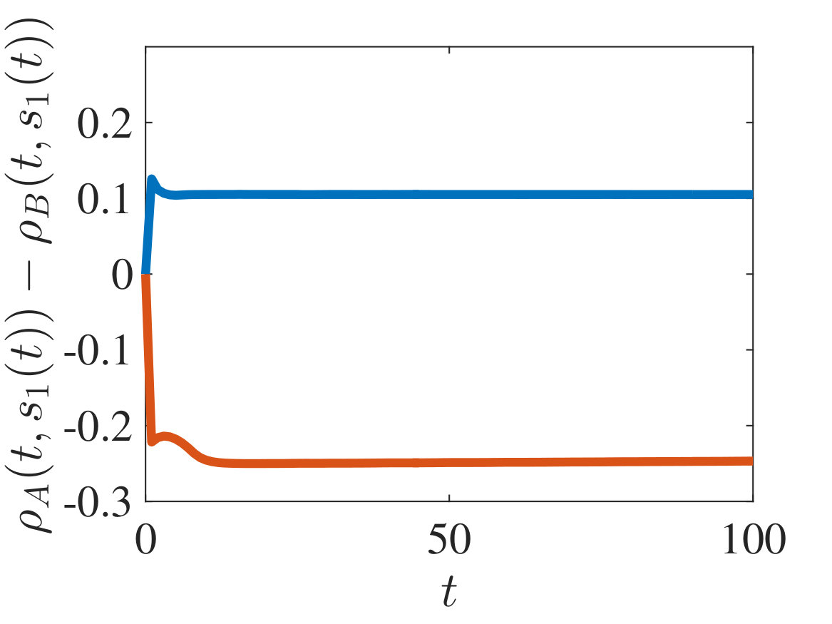 Figure 1
 Figure 2
 Figure 3
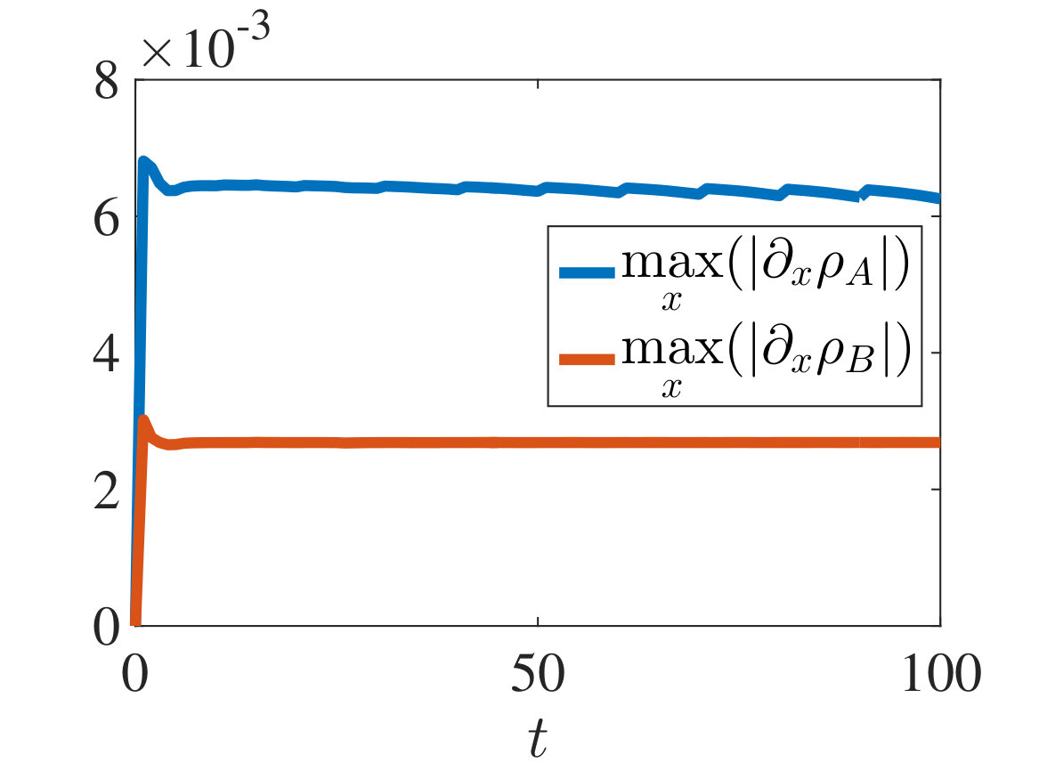 Figure 4
 Figure 5
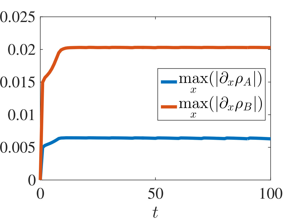 Figure 6
Peer Reviews
No public reviews on file for this paper yet. If you reviewed it on a platform where reviews are public (OpenReview, ICLR, NeurIPS, ICML), you can paste yours below so the community can read it here.
Videos
No videos yet. Explain this paper in a talk, walkthrough, or lecture? Add one.
11footnotetext: accepted in Interfaces and Free Boundaries
[email protected], [email protected], [email protected]
From individual-based mechanical models of multicellular systems to free-boundary problems
Tommaso Lorenzi, Philip J. Murray, Mariya Ptashnyk
University of St Andrews, UK
University of Dundee, UK
Heriot-Watt University, Edinburgh, UK
Abstract.
In this paper we present an individual-based mechanical model that describes the dynamics of two contiguous cell populations with different proliferative and mechanical characteristics. An off-lattice modelling approach is considered whereby: (i) every cell is identified by the position of its centre; (ii) mechanical interactions between cells are described via generic nonlinear force laws; and (iii) cell proliferation is contact inhibited. We formally show that the continuum counterpart of this discrete model is given by a free-boundary problem for the cell densities. The results of the derivation demonstrate how the parameters of continuum mechanical models of multicellular systems can be related to biophysical cell properties. We prove an existence result for the free-boundary problem and construct travelling-wave solutions. Numerical simulations are performed in the case where the cellular interaction forces are described by the celebrated Johnson-Kendall-Roberts model of elastic contact, which has been previously used to model cell-cell interactions. The results obtained indicate excellent agreement between the simulation results for the individual-based model, the numerical solutions of the corresponding free-boundary problem and the travelling-wave analysis.
1. Introduction
Continuum mechanical models of multicellular systems have been increasingly used to achieve a deeper understanding of the underpinnings of tissue development, wound healing and tumour growth [1, 2, 3, 6, 8, 10, 13, 15, 26, 32, 40, 44, 46, 52, 53]. These models are formulated in terms of nonlinear partial differential equations for cell densities (or cell volume fractions) and, as such, are amenable to both numerical and analytical approaches that enable insight to be gained into the biological system under study. From a mathematical perspective, over the past few years particular attention has been paid to the existence of travelling-wave solutions with composite shapes [5, 12, 31, 43, 48] and to the convergence to free-boundary problems in the asymptotic limit whereby cells are represented as an incompressible fluid [7, 30, 33, 41, 42].
Whilst continuum mechanical models of multicellular systems are usually defined on the basis of tissue-scale phenomenological considerations, off-lattice individual-based models enable representation of cell mechanics at the level of individual cells [18, 49]. However, as the numerical exploration of such individual-based models requires large computational times for biologically relevant cell numbers and the models are not analytically tractable, it is desirable to derive continuum models in an appropriate limit [4, 9, 17, 18, 25, 28, 29, 34, 35, 36, 37, 47]. Although mechanical interactions between interfacing cell populations with different characteristics arise in many biological contexts (e.g. tumour growth, development), relatively little prior work has explored the connection between off-lattice individual-based models and continuum models in such situations.
In this paper we propose an individual-based mechanical model for the dynamics of two contiguous cell populations with different proliferative and mechanical characteristics. In our model: (i) every cell is identified by the position of its centre; (ii) mechanical interactions between cells are described via generic nonlinear force laws; and (iii) cell proliferation is contact inhibited. Formally deriving a continuum counterpart of the discrete model, we obtain a free-boundary problem with nonstandard transmission conditions that governs the dynamics of the cell densities. Our derivation extends a previous method developed for the case of a single cell population [36, 37].
To prove an existence result for the free-boundary problem, a novel extension of methods previously developed for related free-boundary problems [21, 22, 23, 51] is required due to the specific structure of our boundary and transmission conditions. In particular, the jump in the density and in the flux across the moving interface between the two cell populations, along with the fact that there are no conditions of Dirichlet type, prevent us from using existing ideas which are partially based on continuity arguments [22, 23] and from applying the enthalpy method [16, 51].
Moreover, building on a recently presented method for a related system of nonlinear partial differential equations [12, 31], we also construct travelling-wave solutions for the free-boundary problem. In this respect, the novelty of our work lies in the fact that we consider a free-boundary problem subject to biomechanical transmission conditions which are different from those considered in [12, 31]. This requires a different approach when studying the properties of the solution at the interface between the two cell populations and introduces a significant difference in the qualitative properties of the travelling wave.
Numerical simulations are performed in the case where the cellular interaction forces are described by the celebrated Johnson-Kendall-Roberts (JKR) model of elastic contact [27], which has been shown to be experimentally accurate in some cases [14], and has been previously used to approximate mechanical interactions between cells [19, 20]. The results obtained support the findings of the travelling-wave analysis, and demonstrate excellent agreement between the individual-based model and the corresponding free-boundary problem.
The paper is organised as follows. In Section 2, we present our individual-based mechanical model and formally derive the corresponding free-boundary problem. In Section 3, we prove the existence result for the free-boundary problem. In Section 4, we develop the travelling-wave analysis. In Section 5, we compare simulation results for the individual-based model and numerical solutions of the free-boundary problem. Section 6 concludes the paper and provides a brief overview of possible research perspectives.
2. Formulation of the individual-based model and derivation of the corresponding free-boundary problem
2.1. Formulation of the individual-based model
We consider a one-dimensional multicellular system that consists of two populations of cells that are arranged along the real line and characterised by different proliferative and mechanical properties. We label the two cell populations by the letters and and make the assumption that, during the considered time interval, the cells in population can proliferate, whereas the cells in population cannot. We denote the number of cells in population by . Moreover, at time we let the function represent the number of cells in population and compute the total number of cells inside the system as .
We adopt a discrete off-lattice modelling approach whereby every cell is identified by the position of its centre [49]. Building upon the ideas presented in [36, 37], we model the two cell populations as a chain of masses and springs with the masses corresponding to the cell centres, and assume the cell order to be fixed. We label each cell by an index and describe the position of the cell’s centre at time by means of the function . Without loss of generality, we let the cells of population be on the left of the cells of population .
We assume that the centre of the first cell of population is pinned at a point , i.e.
[TABLE]
We describe the effect of cell proliferation and mechanical interactions between cells on the dynamics of the multicellular system using the modelling strategies and the assumptions described hereafter.
Mathematical modelling of cell proliferation.
We assume that cell proliferation is contact dependent such that the proliferation rate of the cell in population depends on the position of neighbouring cells, i.e. with . Hence in a time interval the proliferation of cells in population will result in a reindexing of the cell by an amount
[TABLE]
such that
[TABLE]
where .
Mathematical modelling of mechanical interactions between cells.
We make the assumption that mechanical interactions between nearest neighbour cells depend on the distance between their centres. We denote the force exerted on the cell of population by its left and right neighbours by and , respectively, and introduce the parameter to model the damping coefficient of cells in population , where . With this notation and neglecting cell-cell friction, the dynamics of the positions of the cell centres are described via the following system of differential equations
[TABLE]
where and . We complete system (2.4) with the following differential equations
[TABLE]
2.2. Derivation of the corresponding free-boundary problem
In order to formally derive a continuum version of our individual-based mechanical model (2.4) and (2.1), considering the scenario where the number of cells in both populations is large, we introduce the continuous variable so that, for some sufficiently small,
[TABLE]
and
[TABLE]
Moreover, we use the notation
[TABLE]
We assume the function to be continuously differentiable with respect to the variable and twice continuously differentiable with respect to the variable . Under these assumptions, letting and be sufficiently small, and using the Taylor expansions
[TABLE]
along with the approximation
[TABLE]
from (2.3) we obtain
[TABLE]
Moreover, using the Taylor expansions
[TABLE]
and making the additional assumption that the functions and are twice continuously differentiable, we approximate the force terms in (2.4) for as
[TABLE]
Using the approximations (2.7) and (2.8), and combining proliferation (2.3) and mechanical interaction (2.4) processes, we obtain
[TABLE]
and
[TABLE]
Similarly, mechanical interaction processes (2.1) for , and yield, respectively,
[TABLE]
and
[TABLE]
Based on the ideas presented in [36, 37] and according to the considerations given in Remark 2.1, we define the cell number densities of populations and as
[TABLE]
Remark 2.1**.**
The definitions of the cell densities given by (2.13) are based on the observation that, at any time , the quotient of the number of cells in a generic interval , with , and the length of the interval is
[TABLE]
From the above relation, choosing and using the fact that is small, we obtain the following approximate expression for the cell density
[TABLE]
The change of coordinates , with and yields [36]
[TABLE]
Substituting this relation along with the expressions
[TABLE]
into equations (2.9) and (2.10) yields
[TABLE]
and
[TABLE]
Multiplying equations (2.15) and (2.16) by and , respectively, differentiating with respect to , using the fact that
[TABLE]
[TABLE]
with the growth rate of population defined as
[TABLE]
and renaming to , we obtain the following equations for the cell densities and
[TABLE]
where
[TABLE]
Similarly, the evolution equations for the positions of the free boundaries and are obtained from equations (2.11) and (2.12), respectively, yielding
[TABLE]
In order to obtain the boundary conditions (i.e. the conditions at and ) and the transmission conditions (i.e. the conditions at ), that are needed to complete the problem, we consider the mass balance equations
[TABLE]
Using the fact that , together with equations (2.18) and (2.19), yields
[TABLE]
and
[TABLE]
Hence
[TABLE]
and
[TABLE]
The above equations along with equations (2.21) give
[TABLE]
We complement the free-boundary problem (2.18), (2.19) and (2.22) with the following initial conditions for the moving boundaries and , and the cell densities and :
[TABLE]
where . Letting denote the equilibrium cell density (i.e. the density below which intercellular forces are zero) and a critical cell density above which cells stop dividing due to contact inhibition, throughout the rest of the paper we will make the following assumptions:
[TABLE]
[TABLE]
where , and
[TABLE]
Assumptions (2.25) and (2.26), together with notations (2.17) and (2.20), imply that the nonlinear diffusion coefficient and the growth rate are such that
[TABLE]
and
[TABLE]
3. An existence result for the free-boundary problem
Due to the specific structure of our boundary and transmission conditions, the existing well-posedness results for one-dimensional free-boundary problems, such as those presented in [21, 22, 23, 51], are not directly applicable to our problem. Therefore, in this section we prove an existence result for the free-boundary problem (2.18), (2.19), (2.22) and (2.23).
Assumption 3.1**.**
We make the following assumptions on the force terms and , the diffusion coefficients and , the growth rate , and the initial conditions and .
- (i)
The force terms , with , and satisfy (2.25).
- (ii)
The diffusion coefficients , for any , with , are defined by (2.20), satisfy assumptions (2.27), and for .
- (iii)
The growth rate and satisfies assumptions (2.28).
- (iv)
The initial conditions and satisfy assumptions (2.24).
Throughout this section we use the notation
[TABLE]
for , with , and consider solutions in the sense specified by the following definition.
Definition 3.2**.**
A solution of the free-boundary problem (2.18), (2.19), (2.22), (2.23) is given by functions and , with and for , that satisfy equations (2.18) and (2.19), the following boundary and transmission conditions
[TABLE]
the equations for the free boundaries
[TABLE]
and the initial conditions (2.23).
Theorem 3.3**.**
Under Assumptions 3.1 there exists a solution of the free-boundary problem (2.18), (2.19), (2.22) and (2.23).
Proof.
In order to prove the existence of a solution of the free-boundary problem (2.18), (2.19), (2.22) we consider iterations over successive time intervals and use a fixed point argument. In particular, we first show the existence of a solution on a time interval such that
[TABLE]
Subsequently, the boundedness of and , shown at the end of the proof, will allow iteration over successive time intervals in order to obtain an existence result for .
We begin by making the change of variables
[TABLE]
with such that for and for , while for and for , where . The change of variables (3.4) transforms the time-dependent domains and into the fixed intervals and , respectively. A similar change of variables was considered in [21]. Notice that, for and satisfying conditions (3.3), such a change of variables defines a diffeomorphism from into . Hence we obtain
[TABLE]
where and satisfy the reaction-diffusion-convection equations
[TABLE]
complemented with the nonlinear transmission and boundary conditions
[TABLE]
and the equations for the velocities and
[TABLE]
Notice that for ease of notation we denote
[TABLE]
, and the functions are defined in terms of according to (2.20).
In equations (3.5), since for and for , we have
[TABLE]
The assumptions on and , for , ensure that
[TABLE]
Notice that, without loss of generality, we can focus on the case where for . In fact, if the growth term in the equation for would result into and , thus ensuring that due to the transmission conditions at and the convection term in the equation for . In the case where for , using the maximum principle and relations (3.8) we obtain that for . Therefore, we conclude that system (3.6), (3.7), or equivalently system (2.18), (2.19), is nondegenerate. Notice also that assuming with for and , and considering , and as test functions in equations (3.6) and (3.7), one can prove that is continuous in , while and are continuous in for , which is the regularity required to apply the maximum principle. A similar approach was previously used in the analysis of the porous medium equation [50].
The assumptions on imply that
[TABLE]
and, applying the maximum principle to the equation for , we find that has a minimum at and a maximum at . Hence, at for and, therefore, at . Applying the comparison principle and using the fact that for , along with the assumptions on and on the initial conditions, we obtain
[TABLE]
where . Moreover, applying the maximum principle to the equation for and using the assumptions on and on the initial data, along with the boundedness of and the transmission conditions at , yield
[TABLE]
where . Using these results along with the change of variables given by equation (3.4) we conclude that
[TABLE]
If is nonconstant in and for and , the maximum principle yields and . This along with the assumptions on ensures the monotonicity of the free boundaries and , i.e.
[TABLE]
To prove the existence of a solution of problem (3.5)-(3.7) we use a fixed point argument. Let
[TABLE]
which are both well-defined quantities due to the assumptions on and , for . Moreover, consider
[TABLE]
for , some constant , and . Notice that for we have
[TABLE]
Therefore, choosing
[TABLE]
we find that satisfies the conditions (3.3), for , and the change of coordinates (3.4) is well-defined for all .
For some given and , with , we first consider the problem given by the following equations for and
[TABLE]
For and , with , applying the Rothe-Galerkin method and using the a priori estimates obtained by considering as a test function in the equations for , we obtain the existence of a weak solution , with , of problem (3.12). Notice that for , in the same way as below, we can show that the solutions of (3.12) satisfy the regularity properties required by the maximum principle, and obtain that the solutions are bounded and satisfy (3.9) and (3.10), and the equations in (3.12) are nondegenerate.
To derive a priori estimates for and , we consider and as test functions for the equations in problem (3.12). In this way, we obtain
[TABLE]
for , where , , , , , and .
The transmission conditions in problem (3.12) ensure that the integral at is equal to zero, while for the integral at we have
[TABLE]
From the equation for in problem (3.12) we obtain
[TABLE]
Using the definition of and Hölder inequality, the third term on the right-hand side is estimated as
[TABLE]
for any fixed . The assumptions on and , the boundedness of , , and , and the fact that and for , imply
[TABLE]
for . Notice that for we would have the -norm of on the right-hand side of the last inequality. A similar inequality for follows from the equation for in problem (3.12). The Gagliardo-Nirenberg inequality gives
[TABLE]
and, using the fact that is uniformly bounded and choosing sufficiently small, we obtain
[TABLE]
for , where if and if . In a similar way, we also obtain the following pointwise in the time variable estimate
[TABLE]
for a.e. . Additionally, using the Gagliardo-Nirenberg inequality we have
[TABLE]
We shall estimate each term in equation (3.13) separately. Using estimates (3.14) and (3.15) yields
[TABLE]
Notice that assuming the boundedness of , with , we would have the -norm instead of the -norm of in the last inequality. Using the results in (3.15) and (3.17), along with the boundedness of and , we estimate the next term in (3.13) as
[TABLE]
For the fourth integral in (3.13) we have
[TABLE]
for and any fixed . Here we used the following estimate
[TABLE]
along with estimate (3.15). Using (3.17) and the boundedness of we also obtain
[TABLE]
The boundedness of , along with the assumptions on , implies
[TABLE]
for and any fixed .
Thus for and , combining the estimates from above, choosing sufficiently small, and applying the Gronwall inequality yields
[TABLE]
In a similar way we also obtain
[TABLE]
Thus using (3) and (3), along with (3.15) and (3.17), and considering sufficiently small, we find that the map , where is defined as a solution of problem (3.12) for a given , is continuous.
Considering in equation (3.13) instead of and using the boundedness of yield
[TABLE]
and
[TABLE]
for . Choosing sufficiently small, applying the Gronwall inequality, and considering such that
[TABLE]
we obtain the following estimates for and
[TABLE]
The estimate for in terms of and follows directly from differentiating the equation for with respect to and using the boundedness of and , which is ensured by (3) and (3.15). Using (3.20) and (3.15) and differentiating the equation for in (3.12) with respect to , while considering instead of , gives
[TABLE]
Thus for a sufficiently small , or small initial data, is uniformly bounded in and in , for , where
[TABLE]
The Aubin-Lions lemma, along with the Sobolev embedding theorem, ensures that is a compact subset of and of , for . Using inequality (3.17) we also obtain that the embedding is compact. Thus applying the Schauder fixed point theorem, see e.g. [45], gives that for a given pair there exists a solution of problem (3.5) and (3.6) for , with an appropriate choice of .
To complete the proof we shall show that given by
[TABLE]
where for , maps into itself and is precompact. Considering we have
[TABLE]
for an appropriate choice of and . To show that is precompact we consider two sequences and bounded in and obtain
[TABLE]
for , with a constant independent of . Using the fact that the embedding is compact and applying the Aubin-Lions lemma we obtain the strong convergence in , for any , and in as . This combined with the estimate (3.22) ensures that
[TABLE]
as , where we used the fact that
[TABLE]
The convergence in (3) implies the strong convergence in as . Hence, we have proved the existence of a solution of problem (3.5)-(3.7) in with where
[TABLE]
Now we show that and are uniformly bounded, which will allow us to iterate over successive time intervals and obtain that . The uniform boundedness of , the assumptions on , and equations (3.2) ensure that is uniformly bounded. To show the boundedness of , we consider the original problem (2.18), (2.19), (2.22), and (2.23) and apply the comparison principle to the following problem for :
[TABLE]
where and .
Consider the interval , with and the function
[TABLE]
for some . A similar idea was used in [21]. Since and are monotonically decreasing functions, we obtain
[TABLE]
For the derivatives of , since , we have
[TABLE]
Using the assumptions on , for sufficiently small we obtain
[TABLE]
Since is continuous and at , there exists a sufficiently small such that
[TABLE]
Then applying the comparison principle for parabolic equations gives
[TABLE]
Hence we have
[TABLE]
and for some sufficiently small fixed
[TABLE]
Therefore, provided that is uniformly bounded in , for , the uniform boundedness of and allows us to iterate over successive time intervals and prove the existence of a global solution of the free-boundary problem (2.18), (2.19), (2.22) and (2.23).
Thus, as next we prove the uniform boundedness of , or equivalently of , for . First we show higher regularity of the solutions of problem (3.5)-(3.7) by differentiating the equations in (3.5) with respect to the time variable and considering and as test functions, respectively,
[TABLE]
The second term in the equation above can be estimated as
[TABLE]
for . For the third and fourth terms we have
[TABLE]
Moreover,
[TABLE]
We estimate the next terms as
[TABLE]
The reaction term is estimated by
[TABLE]
For the non-zero contributions from the boundary terms we have
[TABLE]
for , where
[TABLE]
and
[TABLE]
Hence, applying the Gronwall inequality and using the estimates (3.20) and (3.21) yields
[TABLE]
with constants , for , depending on and .
Using the Gagliardo-Nirenberg inequality and boundedness of we obtain
[TABLE]
Differentiating (3.5) with respect to the time variable and using definition of , , and yields
[TABLE]
The last term is estimated by
[TABLE]
Similar estimates, using the boundedness of , hold for and . Thus choosing sufficiently small and using the boundedness of and we obtain
[TABLE]
and, considering the same calculations as in the derivation of (3.25), conclude
[TABLE]
where the constant depends on , for , and for .
Hence estimates (3.21) and (3.26) imply that . Since and , for , are bounded, then is bounded in and is bounded in and , for and for a sufficiently small . Taking as test function in (3.5) and using boundedness of and , for , yield
[TABLE]
Considering a cut-off function , such that for and for and for and for and and taking as test function in (3.5) gives
[TABLE]
Therefore, and are uniformly bounded and can be chosen independently of the initial data. Then iterating over , we can conclude that there exists a global solution of problem (2.18), (2.19), (2.22), (2.23).
∎
4. Travelling-wave solutions of the free-boundary problem
In this section, we carry out a travelling-wave analysis for the free-boundary problem (2.18), (2.19) and (2.22).
We begin by noting that under assumptions (2.25), (2.27) and (2.28), the free-boundary problem (2.18), (2.19) and (2.22) can be written in terms of the cell pressures and defined according to the following barotropic relation
[TABLE]
Under assumptions (2.27), the barotropic relation (4.1) is such that
[TABLE]
The monotonicity conditions (4.2) allow one to write both the force terms and the growth rate as functions of the cell pressure , and . Moreover, with the notation
[TABLE]
the monotonicity conditions (4.2) make it possible to reformulate assumptions (2.25) and (2.28) on the functions and as
[TABLE]
and
[TABLE]
Hence, under assumptions (2.25), (2.27) and (2.28), using the barotropic relation (4.1), we can rewrite the free-boundary problem (2.18), (2.19) and (2.22) in the following alternative form:
[TABLE]
Having rewritten the problem in this form allows us to construct travelling-wave solutions using an approach that builds on the method of proof recently presented in [12, 31]. For the sake of brevity, in this section we drop the tildes from all the quantities in problem (4.6).
We construct travelling-wave solutions of the free-boundary problem (4.6) such that both the position of the inner free boundary, , and the position of the outer free boundary, , move at a given constant speed . Without loss of generality, we let go to and consider the case where
[TABLE]
for some , so that
[TABLE]
We make the following travelling-wave ansatz for the cell densities and
[TABLE]
which are related to the cell pressures and through the barotropic relation (4.1). In this framework, substituting the travelling-wave ansatz (4.8) into problem (4.6) we find
[TABLE]
where and denote the derivatives of and with respect to the variable , with . We consider the case where the following condition holds
[TABLE]
which implies . Moreover, we note that the principle of mass conservation ensures that
[TABLE]
for some . The results of our travelling-wave analysis are summarised in the following theorem.
Theorem 4.1**.**
Under Assumptions 3.1(i)-(iii), for any given there exist and such that the travelling-wave problem defined by system (4.9), complemented with the asymptotic condition (4.10), admits a solution whereby:
- (i)
* is decreasing in and satisfies the condition*
[TABLE]
- (ii)
* is decreasing in and satisfies the condition*
[TABLE]
along with the condition (4.11).
Moreover, in the case where , the following jump condition holds:
[TABLE]
Proof.
We prove Theorem 4.1 in five steps.
Step 1: existence of a solution of problem (4.9). For given, we have the following problem for
[TABLE]
Integrating the equation for over , with , and using the condition at we obtain an ordinary differential equation with final condition at , that is,
[TABLE]
which can be solved explicitly giving P_{B}(z)=c\,(\ell-z)+F_{B}^{-1}\Big{(}\dfrac{\eta_{B}}{2}c\Big{)}. Notice that since we have and is invertible. Knowing , we have the following problem for
[TABLE]
Integrating the equation for over , with , and using the second condition at we obtain an ordinary differential equation with final condition at , that is,
[TABLE]
*Under Assumptions 3.1(i), (iii) on the functions , and , the above problem admits a solution. Hence, for a given there exists a solution of problem (4.9). *
Step 2: monotonicity of in and proof of the condition (4.13). Integrating (4.9)2 between a generic point and , and using the boundary condition (4.9)7, we find
[TABLE]
Moreover, integrating (4.15) between a generic point and gives
[TABLE]
Therefore,
[TABLE]
Furthermore, note that (4.15) allows us to rewrite the boundary condition (4.9)6 as
[TABLE]
Since under assumptions (4.4) we have that if and only if , we conclude that
[TABLE]
Finally, since the function is monotone for , cf. (4.4), the value of is uniquely determined by (4.18).
Using the results (4.15), (4.17) and (4.19) along with the fact that, under assumptions (4.1) and (4.2), if and only if and is a monotonically increasing and continuous function of for , we conclude that the function is continuous in and satisfies the following conditions
[TABLE]
and
[TABLE]
Step 3: identification of . For given, since the value of is uniquely determined for all , the value of is uniquely defined by the integral identity (4.11).
Step 4: monotonicity of in and proof of the condition (4.12). Recalling that for , we multiply both sides of (4.9)1 by and use assumption (4.10) to obtain the following boundary-value problem for
[TABLE]
[TABLE]
Let be a critical point of . Using (4.22) we conclude that
[TABLE]
Therefore, under the conditions (4.5) and (4.23), the strong maximum principle ensures that in and that cannot have a local minimum in , i.e.
[TABLE]
Hence the solution of (4.22), (4.23) is a continuous and nonincreasing function that satisfies
[TABLE]
Using the results (4.24) and (4.25) along with the fact that, under assumptions (4.1) and (4.2), if and only if and is a monotonically increasing and continuous function of for , we conclude that the function is continuous in and satisfies the following conditions
[TABLE]
and
[TABLE]
with being related to by (4.3).
Step 5: proof of the jump condition (4.14). The transmission conditions (4.9)4 and (4.9)5 give
[TABLE]
Furthermore, due to the uniqueness of the value of , under the monotonicity assumptions (4.4), the transmission condition (4.9)3 allows one to uniquely determine the value of . In particular, in the case where , the transmission condition (4.9)3 gives
[TABLE]
from which, using the monotonicity assumptions (4.1) and (4.4), one finds the jump condition (4.14). ∎
5. Numerical solutions of the free-boundary problem and computational simulations for the individual-based model
In this section, we illustrate the results established in Theorem 4.1 by presenting a sample of numerical solutions of the free-boundary problem (2.18), (2.19) and (2.22). Moreover, we compare numerical solutions of the continuum model with computational simulations for the individual-based model (2.3)-(2.1). We focus on the case where the force terms and are both given by the following cubic approximation of the JKR force law [27]
[TABLE]
where and stands for the equilibrium intercellular distance, which is the distance between cell centres above which cells do not exert any force upon one another (i.e. for all ). The equilibrium distance and the coefficients , and depend on the biophysical characteristics of the cells and are defined as
[TABLE]
In the formulas (5.2), is the cell radius, the parameter measures the strength of cell-cell adhesion and is an effective Young’s modulus defined as
[TABLE]
with and being, respectively, the Young’s modulus and the Poisson’s ratio of the cells. We refer the interested reader to Appendix A for a detailed derivation of the approximate representation of the JKR force law given by (5.1)-(5.3).
Using the formal relations between the intercellular distance and the cell density (2.13) and (2.14), we compute the cell densities and the equilibrium cell density as
[TABLE]
and . The approximation of the JKR force law (5.1) can be rewritten in terms of the cell densities and as follows
[TABLE]
Inserting the latter expression for into the definition (2.20) of the nonlinear diffusion coefficient yields
[TABLE]
from which, using (4.1), we obtain the following barotropic relation for the cell pressure
[TABLE]
In (5.7), the term is an integration constant such that and
[TABLE]
Numerical simulations were performed using parameter values chosen in agreement with those used in [20], that is,
[TABLE]
where is the density of cell-cell adhesion molecules in the cell membrane, is the Boltzmann constant and is an absolute temperature. Figure 1 displays the plots of the force between neighbouring cells, the nonlinear diffusion coefficient , and the cell pressure , obtained using the parameter values given by (5.9).
We let the cell damping coefficients of population be , and considered the cases where or or . Moreover, for the cell proliferation term we assumed
[TABLE]
where is a smooth approximation to the Heaviside function.
To construct numerical solutions, the free-boundary problem (2.18), (2.19) and (2.22) was transformed to a Lagrangian reference frame and the method of lines was employed to solve the resultant equations. The resulting system of ordinary differential equations, as well as the ordinary differential equations (2.4) and (2.1) of the individual-based model, were numerically solved using the Matlab routine ode15s.
The plots in Figures 2-4 show sample dynamics of the cell density defined as
[TABLE]
with and being either numerical solutions of the free-boundary problem (2.18), (2.19), (2.22) (black lines) or approximate cell densities computed from numerical solutions of the individual-based model (2.3)-(2.1) using (5.4) (red markers). In agreement with the results established in Theorem 4.1, we observe the emergence of travelling-wave solutions, whereby the positions of the inner free boundary and the outer free boundary move at the same constant speed, and the cell densities and are monotonically decreasing.
Moreover, is continuous at if , cf. the plots in Figure 2, whereas it has a jump discontinuity at both for and for . The sign of the jump satisfies condition (4.14), cf. the plots in Figures 3 and 4, and, once that the travelling-wave is formed, the size of the jump is constant and such that the transmission condition (4.9)3 is met, see Supplementary Figure B.1(a). As shown by these plots, there is an excellent match between the numerical solutions of the free-boundary problem and the computational simulation results for the individual-based model.
6. Discussion
We presented an off-lattice individual-based model that describes the dynamics of two contiguous cell populations with different proliferative and mechanical characteristics.
We formally showed that this discrete model can be represented in the continuum limit as a free-boundary problem for the cell densities. We proved an existence result for the free-boundary problem and constructed travelling-wave solutions. We performed numerical simulations in the case where the cellular interaction forces are described by the celebrated JKR model of elastic contact, and we found excellent agreement between the computational simulation results for the individual-based model, the numerical solutions of the corresponding free-boundary problem and the travelling-wave analysis. Taken together, the results of numerical simulations demonstrate that the solutions of the free-boundary problem faithfully capture the qualitative and quantitative properties of the outcomes of the off-lattice individual-based model.
In this paper, we focussed on a one-dimensional scenario where the two cell populations do not mix. It would be interesting to extend the individual-based mechanical model presented here, and the related formal method of derivation of the corresponding continuum model as well, to more realistic two-dimensional cases whereby spatial mixing between the two cell populations can occur. In this regard, an additional development of our study would be to formulate probabilistic discrete mechanical models of interacting cell populations and, using asymptotic methods analogous to those employed, for instance, in [11, 24, 38, 39], to perform a rigorous derivation of their continuum counterparts. These are all lines of research that we will be pursuing in the near future.
Appendix A Approximate representation of the JKR force law
The nonlinear function that gives the JKR force law between the cell and the cell, with centres at distance , is implicitly defined by the following formulas [20]
[TABLE]
where
[TABLE]
In the formulas (A.1), the parameter models the strength of cell-cell adhesion, stands for the radius of the cell, is the Young’s modulus of the cell, and denotes the Poisson’s ratio of the cell. Analogous considerations hold for the parameters of the cell. Moreover, is the sum of the deformations undergone by the cell and the cell.
As the computational cost of numerical simulations carried out by solving implicitly for is prohibitive, we derive an approximate representation of this function based on a third degree polynomial of the form
[TABLE]
with
[TABLE]
In the above equations, denotes the equilibrium distance between the centres of cell and cell (i.e. the distance such that for all ).
With this goal in mind, we look for explicit expressions of , , and in terms of the cell radii and the mechanical parameters of the cells. In the rest of this appendix we will use the abridged notation for .
Expression for .
The equilibrium distance can be directly computed from the formulas (A.1). In fact, choosing and using the fact that , from the second formula in (A.1) we obtain
[TABLE]
Substituting this expression into the first formula in (A.1) yields
[TABLE]
and noting that we find the equilibrium distance .
Expression for .
We substitute the second formula in (A.1) into the first formula to obtain
[TABLE]
where
[TABLE]
Differentiating with respect to yields
[TABLE]
and
[TABLE]
Hence, for we have
[TABLE]
Differentiating both sides of (A.4) with respect to we find
[TABLE]
where
[TABLE]
Rearranging terms in the latter equation yields
[TABLE]
and, therefore, for we have
[TABLE]
Finally, noting that
[TABLE]
we find
[TABLE]
Expression for .
Differentiating twice both sides of (A.4) with respect to yields
[TABLE]
Rearranging terms in the latter equation gives
[TABLE]
Hence, choosing and using the fact that along with the expressions (A.5) for and , we find
[TABLE]
Noting that [cf. the expression of in (A.5)]
[TABLE]
and inserting the expression (A.6) of into (A.7) yields
[TABLE]
Expression for .
Differentiating thrice both sides of (A.4) with respect to yields
[TABLE]
Rearranging terms in the latter equation we obtain
[TABLE]
Hence, choosing and using the fact that , along with the expression (A.7) for and the expressions (A.5) for , and , we find
[TABLE]
where
[TABLE]
Finally, inserting the expression (A.6) for into (A.8) we obtain
[TABLE]
Expressions for , , and .
Taken together the results from above give
[TABLE]
Approximate representation of used to perform numerical simulations.
To perform numerical simulations, we assumed that all cells have the same radius , Young’s modulus and Poisson’s ratio , i.e.
[TABLE]
Under these assumptions, we have that
[TABLE]
and the approximate representation of the JKR force law given by (A.2) and (A.9) reads as
[TABLE]
with
[TABLE]
Appendix B Supplementary figure
The reference list from the paper itself. Each links out to its DOI / PubMed record.
- 1[1] D. Ambrosi and F. Mollica , On the mechanics of a growing tumor , International Journal of Engineering Science, 40 (2002), pp. 1297–1316.
- 2[2] D. Ambrosi and L. Preziosi , On the closure of mass balance models for tumor growth , Mathematical Models and Methods in Applied Sciences, 12 (2002), pp. 737–754.
- 3[3] R. P. Araujo and D. S. Mc Elwain , A history of the study of solid tumour growth: the contribution of mathematical modelling , Bulletin of Mathematical Biology, 66 (2004), pp. 1039–1091.
- 4[4] R. E. Baker, A. Parker, and M. J. Simpson , A free boundary model of epithelial dynamics , Journal of Theoretical Biology, https://doi.org/10.1016/j.jtbi.2018.12.025 (2019).
- 5[5] M. Bertsch, M. Mimura, and T. Wakasa , Modeling contact inhibition of growth: Traveling waves. , Networks & Heterogeneous Media, 8 (2013).
- 6[6] D. Bresch, T. Colin, E. Grenier, B. Ribba, and O. Saut , Computational modeling of solid tumor growth: the avascular stage , SIAM Journal on Scientific Computing (SISC), 32 (2010), pp. 2321–2344.
- 7[7] F. Bubba, B. Perthame, C. Pouchol, and M. Schmidtchen , Hele-shaw limit for a system of two reaction-(cross-) diffusion equations for living tissues , ar Xiv preprint ar Xiv:1901.01692, (2019).
- 8[8] H. Byrne and M. A. J. Chaplain , Growth of nonnecrotic tumors in the presence and absence of inhibitors , Mathematical Biosciences, 130 (1995), pp. 151–181.