Minimax rates for the covariance estimation of multi-dimensional L\'evy processes with high-frequency data
Katerina Papagiannouli

TL;DR
This paper develops a spectral estimator for co-integrated volatility in multi-dimensional Lévy processes using high-frequency data, establishing minimax convergence rates and comparing efficiency with existing methods.
Contribution
It introduces a new spectral estimator for co-integrated volatility and proves its minimax optimality for a broad class of Lévy processes.
Findings
Convergence rates are 1/√n for r ≤ 1 and (n log n)^{(r-2)/2} for r > 1.
The estimator is minimax optimal within the specified class.
The method effectively bounds co-jump activity using the harmonic mean.
Abstract
This article studies nonparametric methods to estimate the co-integrated volatility for multi-dimensional L\'evy processes with high frequency data. We construct a spectral estimator for the co-integrated volatility and prove minimax rates for an appropriate bounded nonparametric class of semimartingales. Given observations of increments over intervals of length , the rates of convergence are if and if , which are optimal in a minimax sense. We bound the co-jump index activity from below with the harmonic mean. Finally, we assess the efficiency of our estimator by comparing it with estimators in the existing literature.
Click any figure to enlarge with its caption.
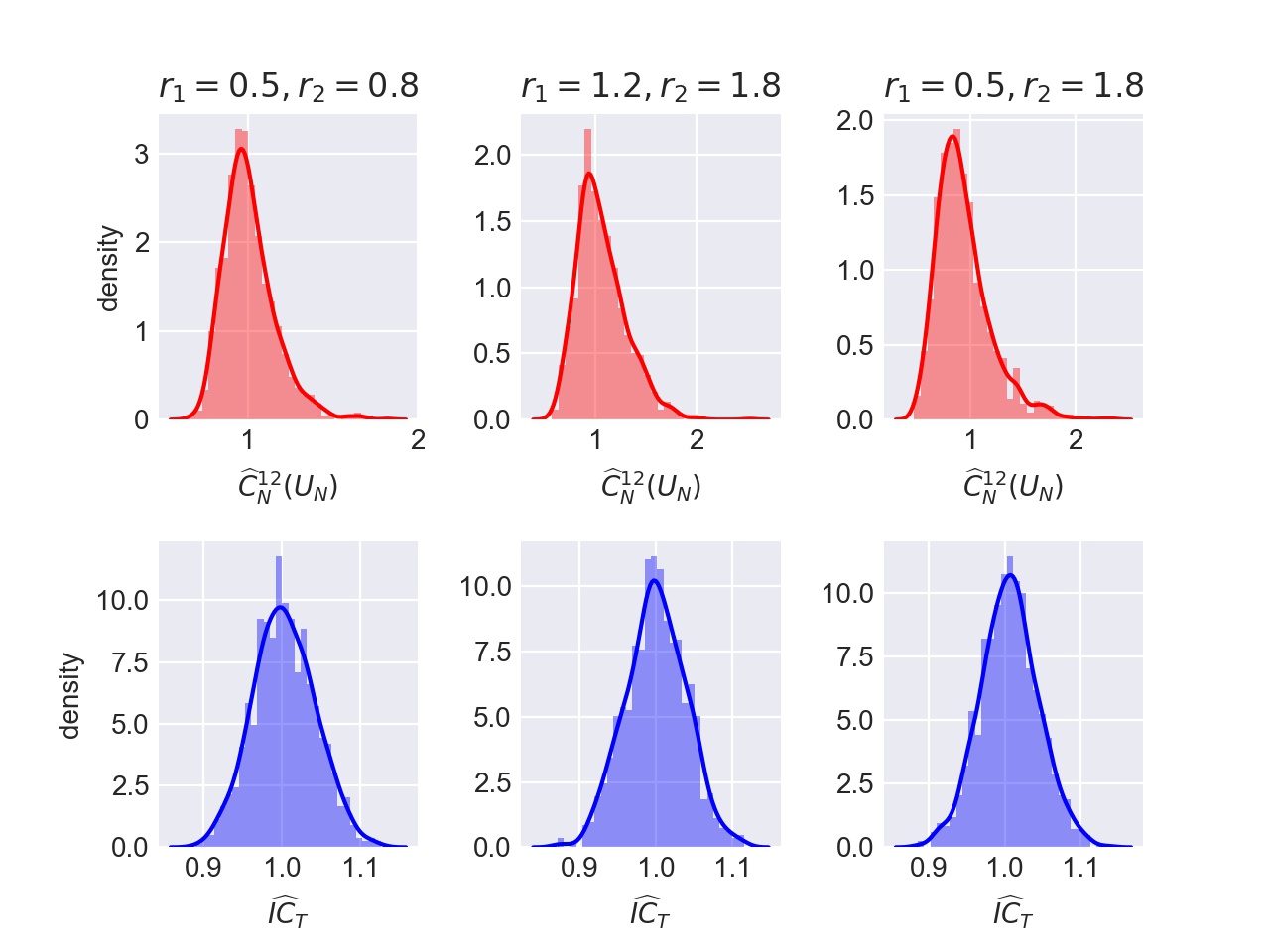 Figure 1
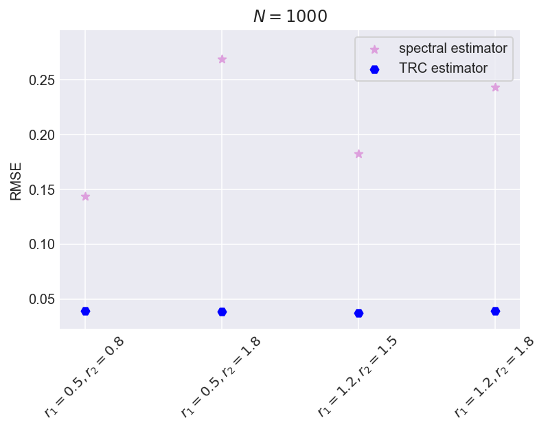 Figure 2
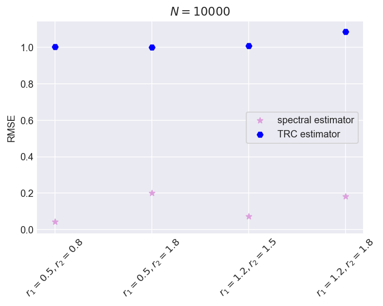 Figure 3
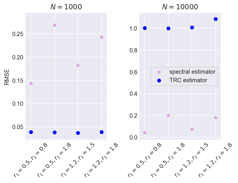 Figure 4
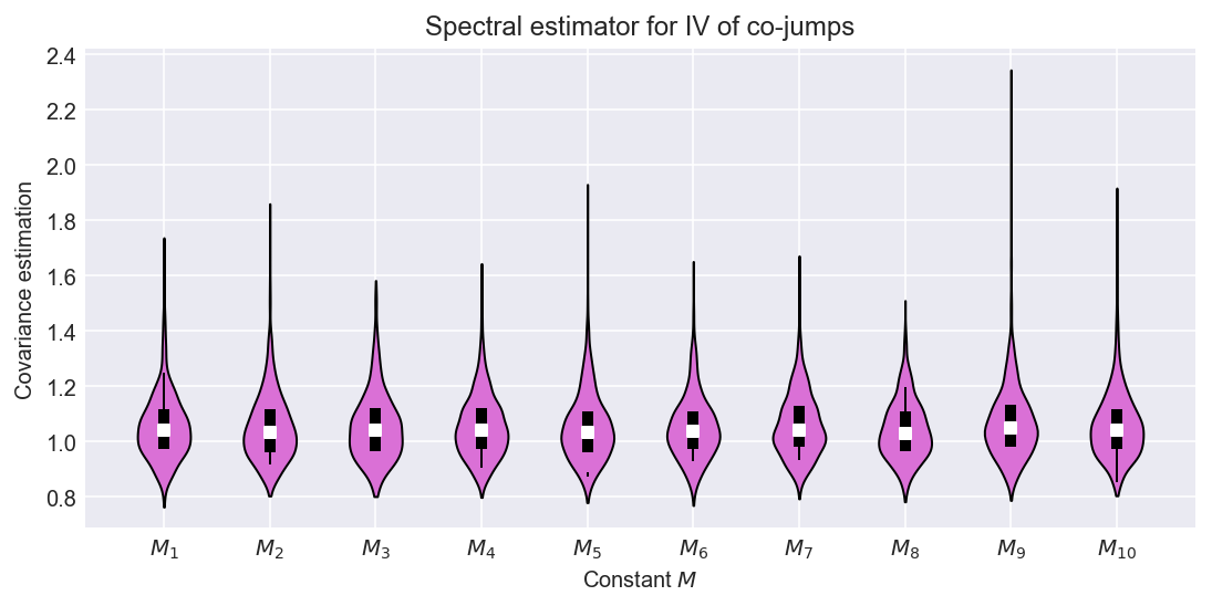 Figure 5
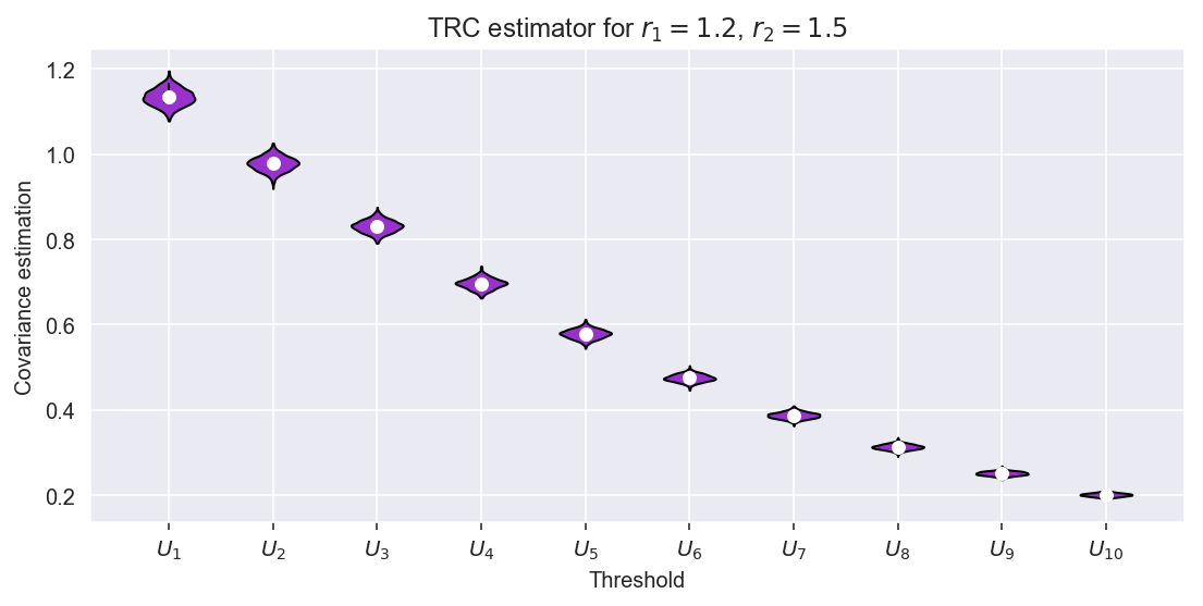 Figure 6
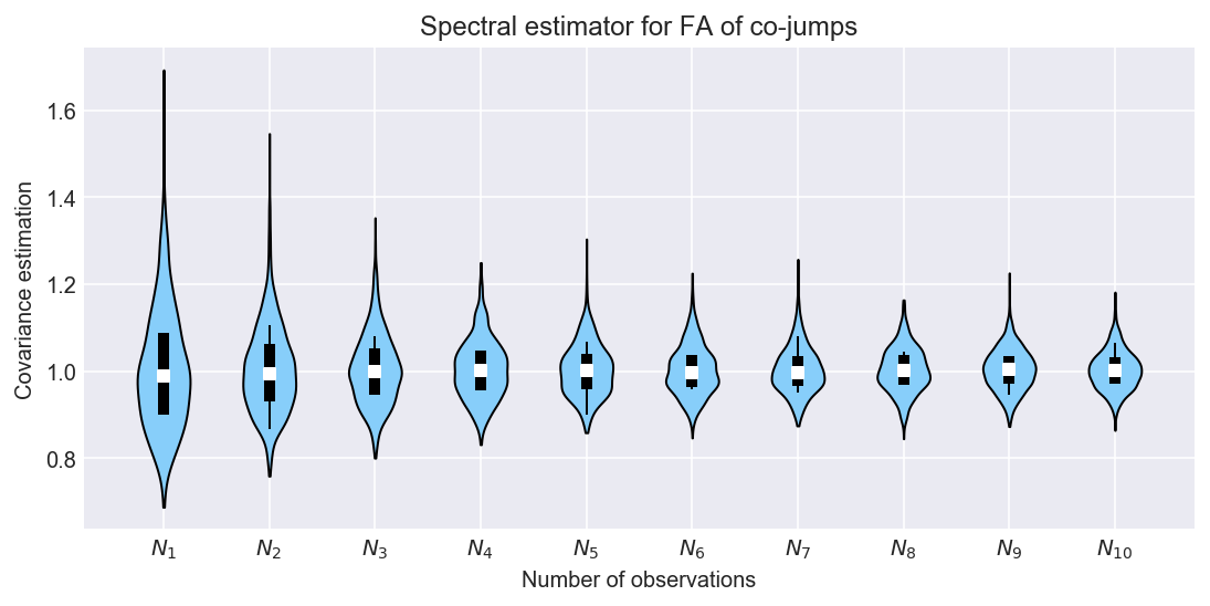 Figure 7
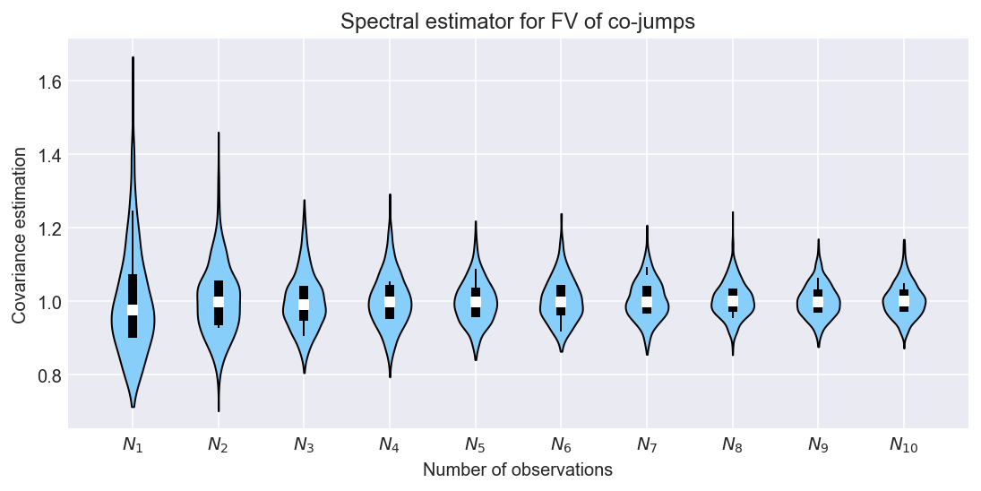 Figure 8
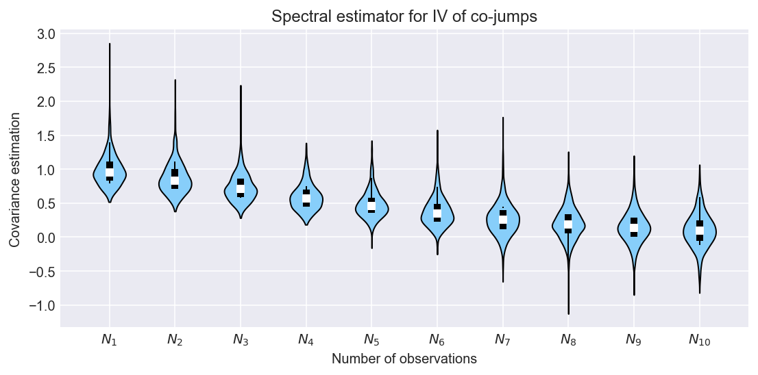 Figure 9
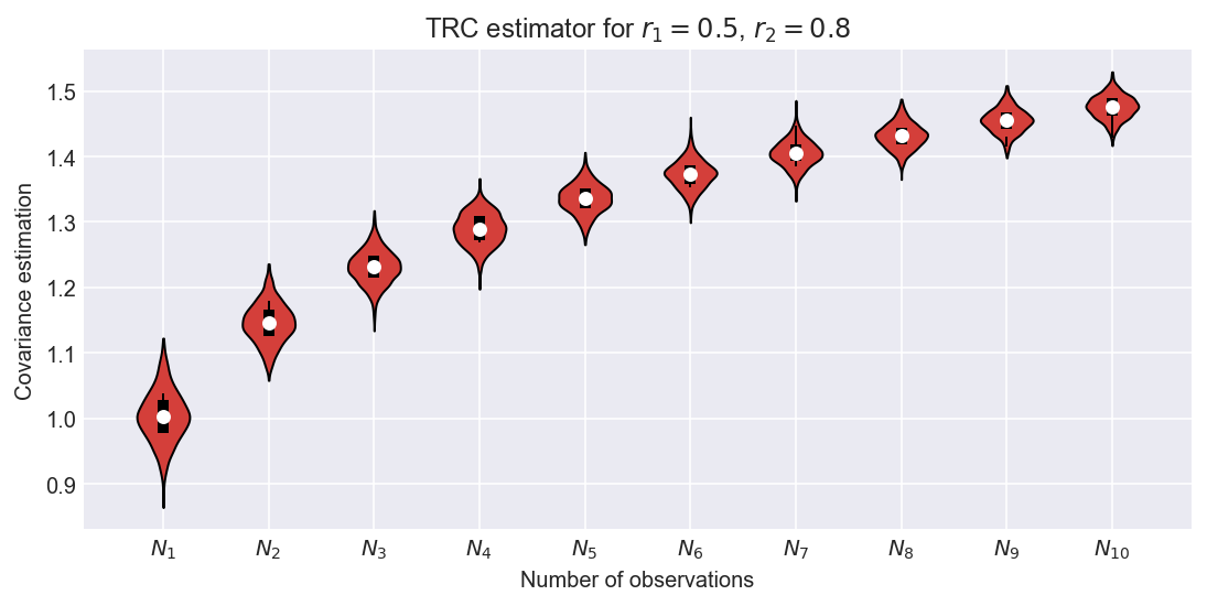 Figure 10
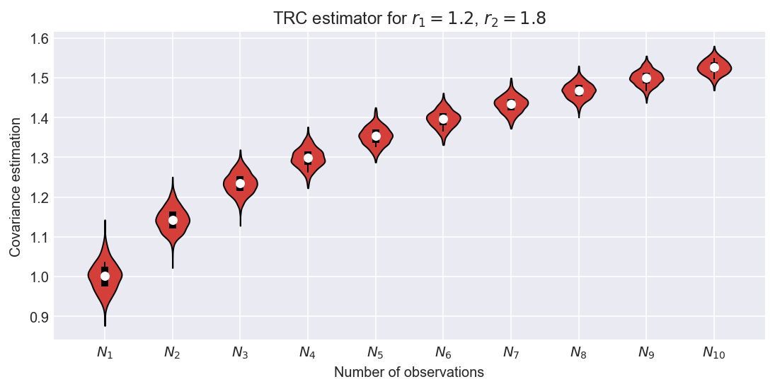 Figure 11
Peer Reviews
No public reviews on file for this paper yet. If you reviewed it on a platform where reviews are public (OpenReview, ICLR, NeurIPS, ICML), you can paste yours below so the community can read it here.
Videos
No videos yet. Explain this paper in a talk, walkthrough, or lecture? Add one.
Minimax rates for the covariance estimation of multi-dimensional Lévy processes with high-frequency data
Katerina Papagiannoulilabel=e1][email protected] [ Humboldt-Universität zu Berlin
Institut für Mathematik
Humboldt-Universität zu Berlin
Unter den Linden 6
10099 Berlin
Germany
Abstract
This article studies nonparametric methods to estimate the co-integrated volatility for multi-dimensional Lévy processes with high frequency data. We construct a spectral estimator for the co-integrated volatility and prove minimax rates for an appropriate bounded nonparametric class of Lévy processes. Given observations of increments over intervals of length , the rates of convergence are if and if , where is the co-jump index activity and corresponds to the intensity of dependent jumps. These rates are optimal in a minimax sense. We bound the co-jump index activity from below with the harmonic mean. Finally, we assess the efficiency of our estimator by comparing it with estimators in the existing literature.
60G51,
62G05,
62G10,
62C20,
60J75,
co-jumps,
infinite variation,
co-integrated volatility,
high-frequency data,
keywords:
[class=MSC]
keywords:
\startlocaldefs
1 Introduction
Lévy processes are the main building blocks for stochastic continuous-time jump models. Whenever the modeling of a stochastic process in finance requires the inclusion of jumps, Lévy processes are those to be considered. They play an instrumental role, for example, in the modeling of financial data, see Carr et al. (2002); Barndorff-Nielsen and Shephard (2004, 2006); Wu (2007); Eberlein and Papapantoleon (2005); Geman (2002).
Consequently, the large amount of applications has given rise to a great demand for statistical methods in the study of Lévy processes, especially nonparametric methods. Using nonparametric methods relaxes any dependency on the model. The problem of estimating the characteristics of a Lévy process has received considerable attention over the past decade. Starting with the work by Belomestny and Reiß (2006), a number of articles have considered nonparametric estimation methods for Lévy processes. Therefore, one important task is to provide estimation methods for the characteristics of a Lévy process.
Moreover, statistical methods require the nature of the observation schemes to be classified as high frequency or low frequency; here, we focus on a high frequency setting. If we can assume high-frequency observations for a Lévy process, we can discretize a natural estimator based on continuous-time observations, where the jumps and the diffusion part are observed directly. In recent years, the literature on this subject has grown extensively, see Figueroa-Lopez and Houdré (2004); Todorov and Tauchen (2011); Coca (2018); Comte and Genon-Catalot (2009); Neumann and Reiß (2009). We now have vast amounts of data on the prices of various assets, exchange rates, and so on, typically tick data which are recorded at every transaction time.
Much has been written on the estimation of Lévy density using nonparametric techniques, for instance Nickl et al. (2016), Duval and Mariucci (2017), Comte and Genon-Catalot (2014) and the references therein. However, we are interested in the estimation of the continuous part of a Lévy process, although jumps still play a central role in this estimation. In the univariate context, the seminal work of Andersen and Bollerslev (1998) and Barndorff-Nielsen and Shephard (2002), proposed realized variance as an estimator for quadratic variation. In the presence of jumps, a well-known theoretical result proves that the realized variation converges in probability to the global quadratic variation as the time between two consecutive observations tends towards zero. This result motivated estimators that filter out the jumps, like Bipower Variation by Barndorff-Nielsen and Shephard (2004) and Truncated Realized Variation by Mancini (2009).
In the multivariate context, the recovery of co-integrated volatility (also known as covariance) becomes more complicated. Among various prominent works see Christensen et al. (2013), Bibinger and Vetter (2015), Bibinger and Winkelmann (2015). For models incorporating jumps, the realized covariation converges in probability to the global quadratic variation containing the co-jumps. Co-jumps refer to the case when the underlying processes jump at the same time with the same direction. This raises the question how we can assess the dependent structure among the jump components. We find the answer in the Lévy copula, a subject studied by Tankov (2004) in his PhD thesis. The interested reader should refer to Tankov and Cont (2003) and Kallsen and Tankov (2006). The Lévy Copula is the basic tool for the class of multidimensional Lévy processes. To mention only the few approaches which are close to our focus on Lévy processes we refer to Mancini (2017), Christensen et al. (2013), Martin and Vetter (2017), Bibinger et al. (2014), Jacod and Reiß (2014), Bücher and Vetter (2013) and Belomestny and Trabs (2018).
Our aim in the present work is to provide minimax rates of convergence for the estimation of co-integrated volatility when the underlying process belongs to a certain class of multi-dimensional Lévy processes. Many features of co-integrated volatility have already been studied, such as asynchronous observations, microstructure noise, and allowing for dependency among the jumps components. Whereas most of the aforementioned results prove central limit theorems for their estimators, at least to the best of our knowledge no work has dealt with optimal rates of convergence in the minimax sense. This work serves to fill this gap. Jacod and Reiß (2014) proposed a spectral estimator for integrated volatility achieving minimax rates. In the present work, we generalize their work on finite dimensions. By virtue of simplicity, we will concentrate primarily on a two-dimensional regime, but extensions to the general multi-dimensional setting are straightforward to obtain as well.
For this purpose let us define, for a two-dimensional Lévy process X, the Blumenthal- Getoor index :
[TABLE]
where is the size of the jump components, is the Euclidean norm in , is the Lévy measure. is not specifically interesting but the - index gives us the infimum number for which is finite. This index is a very important number for the Lévy processes, because using this index we can infer about the behavior of small jump components around [math]. When we have a two-dimensional Lévy process we have either independent jumps (i.e. disjoint or jumps in the axes) or dependent (i.e. co-jumps or joint jumps). In the present work we focus on the case of co-jumps, when the two marginals jump at the same time in the same direction. So the index gives us information about the amount of disjoint and joint small jumps around [math]. The behavior of co-jumps around [math], is described by
[TABLE]
Here, we are interested in investigating the optimal rates for the estimation of co-integrated volatility when the model falls in a class of two-dimensional Lévy processes, in case the jump components are either of finite or infinite variation and satisfy (1.2). Let and , be the index of jump activity for the small jump components of each process respectively. We find that , the index activity of co-jumps, is bounded from below by the harmonic mean of , even in the case of infinite variation jumps. This was not known up to now. Under this assumption for co-jumps we show that our spectral estimate for co-integrated volatility converges at a rate if and if .
Assuming a 2-dimensional Itô semimartingale, Mancini (2017) proposed a truncated covariance estimator to estimate co-integrated volatility at the rate when is small and is close to 1, n^{-\frac{1}{2}\big{(}1+\frac{r_{2}}{r_{1}}-r_{2}\big{)}} when is much bigger than and close to , n^{\big{(}\frac{r_{2}}{2}-1\big{)}} when is small and is much bigger than or in case of independent small jump components. However, these rates are sub-optimal for the class which we described in the last paragraph .
Let us describe the outline of this paper. In Section 2 we state the underlying model. In Section 3 we give the assumptions to be satisfied in order to prove the minimax rates. In Section 4 we construct our spectral estimator and state the results of this work. Section 5 gives the insight behind the co-jump index activity. In Section 6 we prove the upper bound for the family of our estimators. In Section 7 we present the proof of lower bound in a minimax sense. We provide some comparison of our estimator with existent estimators in the literature in Section 8. In the last section we provide a simulation study.
2 The underlying model
We assume equidistant discrete observations with the consecutive time between two observations being for a mesh . Here, we use as a mesh and . Regarding the time horizon of the process, it is observed on a finite time span . Let be a two-dimensional Lévy process with Lévy-Itô decomposition as
[TABLE]
Unless stated otherwise, from now on b is a drift vector in , denotes a bivariate Brownian motion with covariance matrix , and are the jump measure and its compensator, respectively. The compensator takes the form , where is the Lévy measure of X.
Due to the independence of the continuous part and the discontinuous (jump part) of a Lévy process, the analysis of X canonically splits into the inference on the covariance matrix and the inference on the jump measure . Our focus on this paper is to investigate an estimator for the co-integrated volatility of X.
We assume a filtered space supporting two independent standard Brownian motions and two Poisson random measures for on . Recall that are correlated with , where is a constant on . We construct as a linear combination of the two independent Brownian motions so . Next we calculate the variances and covariance of , we see that the following holds
[TABLE]
[TABLE]
For the covariance we obtain
[TABLE]
the last equality holds because of being independent. So, without loss of generality we assume that
[TABLE]
where are deterministic. Therefore, the global quadratic variation of X is given by:
[TABLE]
where the first term is the co-integrated volatility and the second term is the sum of products of simultaneous jumps (called co-jumps). Our target of inference, the co-integrated volatility at time , is
[TABLE]
3 Assumptions
To derive an estimator for co-integrated volatility and then prove minimax bound for this estimator, we need to establish some assumptions regarding the behavior of small jumps and the class of our estimator. In particular, our setup is intrinsically nonparametric and related to the properties of the observed path. We use the following notation for a matrix: is the maximum absolute row sum of the matrix, (i.e. the -norm).
Assumption (1-M)**.
The -norm of the covariance matrix is assumed to be bounded, i.e. .
Assumption (2-M)**.
, where .
Notice that Assumption Assumption (2-M) follows from the classical condition to control the activity of small jumps in two dimensions. Through a trivial calculation
[TABLE]
By using this unconventional Assumption Assumption (2-M), we relax the classical condition for small jumps in two dimensions and make our results stronger, since we consider the case of dependent jumps.
Assumption Assumption (2-M) concerns the behavior of jump components with size smaller or equal to one. By this assumption we consider the problem of controlling the activity of co-jumps, i.e. joint jumps. Below, a co-jump, say at time , means that both components jump at this time but their jump sizes may not be the same. Ultimately, we are asking that is to say if the small jump components are of finite or infinite variation. This question concerns the behavior of the compensator , the Lévy measure, near 0. The major difficulties here come form the possibly erratic behavior of near [math] and the possible dependence between the jump components. In Section 5 we describe more detailed the dependence structure of the jump components and the co-jump index activity .
The Blumenthal-Getoor (BG) index allows us to classify the processes from least active to most active, according to the above description. We denote by the BG index for a two-dimensional Lévy process which satisfies:
[TABLE]
Note that a stable Lévy process of index satisfies for all , but not for . The BG index of a - stable is exactly .
The problem of BG index estimation from discrete observations of a Lévy process has drawn much attention in the literature. In the case of high-frequency data, Aït-Sahalia and Jacod (2011) studied the problem of estimating the jump activity index that is defined for any Itô semimartingale. A consistent estimator for the BG index based on one-dimensional Lévy processes with low-frequency data was obtained in Belomestny (2010). The interested reader should refer to Belomestny and Reiß (2015), Section 7 for a detailed review of these results. An extension to time-changed Lévy processes can be found in Belomestny and Panov (2013a, b).
Now we will test the Assumption Assumption (2-M) about the boundedness of small co-jumps with some trivial examples. Despite its simple nature, the following example offers significant insight and intuitive understanding into co-jumps with infinite variation.
Example 3.1**.**
Suppose we have independent jumps in the coordinates and is a Lévy measure on and x is a vector in . Then, which means that
[TABLE]
if the marginals of a two-dimensional Lévy process are finite in the one dimensional case, see the assumption section in Jacod and Reiß (2014).
In this example, we notice that
[TABLE]
since the integrand is always equal to zero. This means that the deterministic error of our estimator is equal to zero, see Section 6.2 for further details. This example shows us something more: Whenever we have independent jumps, no matter the choice of , we can always find a control for the activity of small jumps. Even if we have jumps of infinite variation.
Example 3.2**.**
Suppose we have independent jump size distribution, which means that , so
[TABLE]
if and only if for and the Assumption Assumption (2-M) holds.
4 Theoretical results
We use standard notation for asymptotic quantities like if is stochastically bounded (i.e. bounded in probability or tight). We are in a nonparametric setting in which the process X belongs to the class . Let us now define this class.
Definition 4.1**.**
For and , we define the class , the set of all Lévy processes, satisfying
[TABLE]
We adapt an estimator proposed by Jacod and Reiß (2014). Specifically, we let X be a two-dimensional Lévy process with characteristic triplet . Let us remember that we are in a high-frequency setting and the consecutive time between two observations is . The characteristic function of is given by:
[TABLE]
where is the covariance matrix and . In the same vein, we define the characteristic function where . Here, we focus on estimating the characteristic function on the diagonal of first and fourth quadrant for sake of simplicity to our calculations. The results still hold even when we move away from the diagonal. Following a trivial calculation we get that
[TABLE]
[TABLE]
So, the covariance is given by
[TABLE]
We consider, based on the observations, the empirical characteristic function of the increments, at each stage n:
[TABLE]
Similarly, we consider the empirical characteristic function. Based on the trivial calculation (4.3), we now define the spectral estimator
[TABLE]
The first result of this paper is the following theorem.
Theorem 4.2**.**
Let X belong to the class . Assume and , then as the family of estimators with
[TABLE]
satisfies within the class where
[TABLE]
Particularly, we have that the family of estimators is consistent with the theoretical co-integrated volatility with the exact rates of convergence .
Theorem 4.2 gives us an upper bound for the family of our estimators . In Section 6, we give a proof of the upper bound for the family of our estimators . Let us finally show that on the class the rate (4.6) can be achieved exactly and thus constitutes the exact minimax optimal rate.
Theorem 4.3**.**
Let X belong to , and . Then there are constants such that
[TABLE]
where is any estimator for the co-integrated volatility and is the euclidean distance on .
Theorem 4.3 gives us a lower bound for the family of our estimators within the class . The rates (4.6) for estimating , namely the co-integrated volatility at time are optimal in a minimax sense. In Section 7 we prove this result.
5 Co-jump index activity
We are interested in bounding from below the co-jump activity in the case that at least one of the jump components is of infinite variation. Each component of a two-dimensional Lévy process has its own index activity for . In the following we will describe the method for bounding from below the index activity of co-jumps. The BG index of a Lévy process depends only on the Lévy measure . is an index taking care of positive and negative jumps, for simplicity’s sake but without loss of generality we develop our method for the case in which the Lévy measure is one-sided, i.e. only makes positive jumps. Thus, will be influenced by the dependent structure between the jump components.
We will use a Lévy copula to describe this dependency. The concept of Lévy copula allows us to characterize in a time-independent scheme the dependence structure of the pure jump part of a Lévy process. Here, we use the Lévy copula, which permits a range from a dependent to a total independent framework. For the definition and concepts of independence and total positive dependence copula we refer to Kallsen and Tankov (2006). The next definition is taken from Mancini (2017).
Definition 5.1**.**
The occurrence of joint jumps in is described by the following tail integrals
[TABLE]
where is a Lévy copula of the form
[TABLE]
where is the independence copula, is the total positive dependence copula and varies in .
The following remark gives us some clarifications on the definition of the above Lévy copula.
Remark 5.2*.*
The marginal tails are defined on , the joint tail is defined on . stands for , and is allowed: both could be , namely when both . In that case is , and . is a Lévy copula because it is a convex combination of two Lévy copulas, i.e. is a increasing, grounded and with uniform margins, because and are such. is not a tail integral, it has different properties, for instance , while for any tail we have Finally, when jump components are totally dependent while when the opposite (ask Jacob).
We observe that the index activity of co-jumps is bounded from below by the harmonic mean.
Lemma 5.3**.**
Suppose that Assumption Assumption (2-M) holds. Let be an one-sided -stable Lévy process for with positive jumps. Given assume without loss of generality and . We assume either complete dependent or independent jumps. Then, we have that
[TABLE]
where is the index activity of co-jumps.
Proof.
Each is following a -stable Lévy process with Lévy measure
[TABLE]
for each . We assume without loss of generality that . We denote by
[TABLE]
the tail integral of the marginal Lévy measure . Note that is the BG index of .
The independent jumps have sizes of either or . This means that we have jumps only on the Cartesian axes. The independent copula regulates such jumps. On the other hand, the complete dependent jumps are regulated by the dependent copula; their size falls into the point . The complete dependent jumps are completely positively monotonic, i.e. there exists a strictly increasing and positive function such that , . This means that when is a jump realisation so there is a realisation such as , then is interpreted as the first component of the joint jump. In fact, the sizes are supported by the graph . For the dependent copula we need the minimum between and , which is attained when . Hence, the graph supports the joint jumps.
In our case we assume one-sided -stable processes, which means that the union graph of the joint jumps is given by . We denote by the Lévy measure in terms of the Lévy copula, using the Definition 5.1. Therefore,
[TABLE]
Observe that , since the independent copula regulates the jumps on the axes. Inserting (5.1) into Assumption Assumption (2-M), it turns out that for smaller than , we get
[TABLE]
The first equality holds because of the fact that the integrand is always equally to zero in case of independent jumps. For sake of simplicity, we assume , i.e. totally dependent jumps. We assume that the jump sizes falls into the interval for sufficiently small . Remember and , then we have , which implies \epsilon\geq U_{2}^{-1}\big{(}U_{1}(\epsilon)\big{)}=f(\epsilon). Since we want to bind and , this gives us . Hence,
[TABLE]
where C=\Big{(}\frac{c_{1}r_{2}}{r_{1}c_{2}}\Big{)}^{-\frac{1}{r_{2}}}.
In light of the above calculations, in order for the integral in (5.3) not to be divergent we need \Big{(}\frac{r_{1}}{r_{2}}+1\Big{)}\frac{r}{2}-1-r_{1}>-1, which means that . We observe that , the index activity of co-jumps, is at least the harmonic mean of the indices . In addition, , since we assume . To conclude, the Blumenthal-Getoor (BG) index of the co-jump activity will be bounded from below by
[TABLE]
The proof now is complete. ∎
We see here that the higher the activity of one jump component, the higher the activity of co-jumps.
Next we proceed to the proof of the upper bound Theorem 4.2 using a spectral estimate for the co-integrated volatility. Given the fact that we know an estimate for the integrated volatility , we should consider a straightforward estimate for co-integrated volatility. By polarization, is a possible estimator for the co-integrated volatility. However, we refrain from using this estimate because the rates of convergence are slower than following the procedure as in Section 6. Let us illustrate this argument with an example.
Example 5.4**.**
Let be a Lévy process with characteristic triplet , i.e., without a Gaussian part. We assume its components are independent stable Lévy processes for such that and . Using Lemma 4.1 from Kallsen and Tankov (2006) F is supported by the coordinates axes and it can be written as . The Lévy measures of the components are
[TABLE]
More precisely,
[TABLE]
In order the integrals in the last equality not to be divergent we need and . As a consequence, we find that . Using (3.1) we find that the Blumenthal-Getoor index .
6 Upper Bound
In this section we prove Theorem 4.2. We say that a sequence of estimators achieves the rate on , for estimating , if . This means that the family is tight. Note that the argumentation in line is the bias-variance decomposition.
6.1 The bias-variance decomposition
We start with deriving a bias-variance-type decomposition of the estimation error of the estimator for cointegrated-volatility.
Lemma 6.1**.**
We have that
[TABLE]
The deterministic error given as
[TABLE]
and the stochastic error as
[TABLE]
Proof.
We set C_{n}^{12}(U_{n})=\frac{n}{2U^{2}_{n}}\bigg{(}\log|\phi_{n}(\tilde{\textbf{u}}_{n})|-\log|\phi_{n}(\textbf{u}_{n})|\bigg{)}, recalling the form of the estimator (4.5). We get
[TABLE]
Inserting (4.5) into (6.3), we get that estimation error is given by . We need both quantities to be different than zero, otherwise the estimation error does not hold. ∎
Our goal is to show that the estimation error is stochastically bounded, i.e. . Firstly, we bound the deterministic error.
6.2 Bounding the deterministic error
Lemma 6.2**.**
Grant Assumption Assumption (2-M). The deterministic error satisfies , where is a positive constant.
Proof.
Recall the characteristic function of in (4.2). We define
[TABLE]
Therefore,
[TABLE]
and |\phi_{n}(\tilde{\textbf{u}}_{n})|=\exp\left(-\frac{1}{2n}\bigg{(}\left\langle C\tilde{\textbf{u}}_{n},\tilde{\textbf{u}}_{n}\right\rangle+\tilde{d}_{n}\bigg{)}\right). Notice that here we use an argument of complex analysis. After taking the absolute value of the characteristic function, the imaginary part of the exponent is vanishing. Summing up,
[TABLE]
By (6.6), we have
[TABLE]
where we used the fact that . Using the inequality for , the last term can be bounded as follows
[TABLE]
here because is the co-jump index activity. By Assumption Assumption (2-M) and for some constant ,
[TABLE]
as required. ∎
6.3 Bounding the stochastic error
We want to investigate how close the empirical characteristic function is to the characteristic function of a two-dimensional Lévy process. The variables are i.i.d. as varies, with expectation . The same statement holds true for as well. So is an unbiased estimator because . Also, the variance of the empirical characteristic function is given by .
Definition 6.3**.**
For a - valued random variable we define
[TABLE]
Lemma 6.4**.**
Let and , where . Then, and .
Proof.
Set such that . Remember that is unbiased due to the fact that , thus . Taking this into consideration with the previous definition (6.3), we obtain that . Therefore,
[TABLE]
The same argument holds also for . This completes the proof. ∎
We choose \textbf{u}_{n}=\big{(}U_{n},U_{n}) and . Recall that we estimate the characteristic function on the diagonal of first and fourth quadrant for calculation simplicity. Particularly, we choose for , and large enough
[TABLE]
Lemma 6.5**.**
Grant Assumption Assumption (1-M). For some positive constants and on the event the stochastic error satisfies:
[TABLE]
Proof.
Recalling the form of stochastic error (6.2), the first quantity we need to bound is:
[TABLE]
The first inequality holds because
[TABLE]
using the Cauchy-Schwarz inequality for and the fact that . The last inequality in (6.12) derives from AssumptionAssumption (1-M) and the fact that we always have . Next, the form of (6.10) implies that
[TABLE]
where . Let us now argue that
[TABLE]
as soon as and by (6.13) on the set and . Therefore, . Accordingly, for the stochastic error on the events and we obtain for some deterministic constant :
[TABLE]
In the last inequality, we use the linearized stochastic errors for because of the fact that and are small enough. So there is a positive constant such that . Therefore,
[TABLE]
Henceforth, for , and for some constant , we have
[TABLE]
The third inequality holds because we applied the Cauchy-Schwarz inequality and by Lemma 6.9. To sum up, by (6.13) we get that
[TABLE]
as required.
∎
Remark 6.6*.*
Here, we are interested in the events and because the probabilities of the events and are negligible. Indeed, applying the Chebyshev inequality and by Lemma 6.9 we get
[TABLE]
which tends towards zero as . Likewise, the probability of the event tends towards zero as .
Until now we bound from above the deterministic and stochastic errors. We are now ready to prove that the family is tight in and thus establish an upper bound for our estimator.
End proof of Theorem 4.2
Applying the Markov inequality, we get for every
[TABLE]
Further applying Lemmas 6.5 and 6.2, we deduce that, as
[TABLE]
for (6.18) smaller than , proves that the family is tight in . The proof is complete.
7 Lower Bound
In nonparametric statistics it is common to use a minimax approach in order to prove optimal estimators. In the previous section, we proved Theorem 4.2, which gave us an upper bound for the estimation of co-integrated volatility using a spectral approach and establishing the rates (4.6) on the class .
In this section, we want to prove Theorem 4.3. The existence of a lower bound on the class constitutes the exact minimax rates for the estimation of co-integrated volatility. Indeed, we have something more for the lower bound, namely that any estimator on a general class of Itô semimartingales satisfying Definition 4.1 achieves a lower bound with rates (4.6). So far, we do not know whether the spectral approach for the upper bound yields the same optimal rate on the larger class of Itô semimartingale.
We refer to Chapter 2 in Tsybakov (2009) for the techniques to prove the lower bounds. We establish the lower bound following the argumentation in line with a two-hypothesis test. Next, we introduce a distance between probability measures that will be useful for the lower bound.
Definition 7.1**.**
The total variation distance between is defined as follows:
[TABLE]
where , and a -finite measure.
To sum up, in order to prove a lower bound on the minimax probability of error for hypotheses we use the theorem [2.2] in Tsybakov (2009). The lower bound is obtained when the following two properties are satisfied. First, we choose the appropriate parameters for the co-integrated volatility to be close enough but distinguished. Second, we bound from below the total variation distance between the two densities probabilities of our parameters.
Let us illustrate the above procedure giving a trivial lemma and proving that the above arguments are adequate, so as to obtain the lower bound corresponding to our family of estimators . The interested reader may refer to Lehmann and Romano (2006) who explore a lot of examples for hypothesis testing and distances between Gaussian random variables.
Lemma 7.2**.**
(No jumps for a two-dimensional Lévy process). Assume X belongs to the class with Lévy-Khintchine triplet . Then there are constants such that
[TABLE]
where is any estimator for the co- integrated volatility withing the class , is the euclidean distance on and .
Proof.
Consider X and Y belongs to . Also, we assume that no jumps are occurred so the Lévy Khintchine triplets for each process will satisfy and respectively. As a result, X will evolve as follows:
[TABLE]
[TABLE]
similarly for Y. We know that the Itô integral is normally distributed with mean [math] and its variance is given by Itô isometry which translates to
[TABLE]
Therefore, X follows the parametric model
[TABLE]
similarly for Y.
We will prove the lower bound using the two-hypothesis test, as mentioned in the beginning of this section. We observe that
[TABLE]
where is the class of all Brownian motions where the covariance matrix is bounded component-wise by a constant . As a consequence,
[TABLE]
This is enough to prove a lower bound for the rate for the class of all Brownian motions.
The two-hypothesis test is the following
vs
where the covariance matrices are given by and . Intuitively, we perturb the off-diagonal elements, namely the covariance, by the rate we want to achieve. Following the argumentation of the two-hypothesis test, it is sufficient to prove that the total variation distance is bounded. To do so, we use the Pinsker inequality. By Pinsker inequality we have that
[TABLE]
where is the Kullback-Leibler divergence. Next, we show that the Kullback-Leibler distance is bounded. We define the Kullback-Leibler divergence between two multivariate normal distributions. Here, we denote by and . Therefore,
[TABLE]
where denotes the determinant of a matrix. Calculating the appropriate quantities, we obtain
[TABLE]
[TABLE]
[TABLE]
Therefore,
[TABLE]
Consequently, we obtain that the right hand side tends to zero as . By Pinsker inequality, the total variation distance tends to zero. Upon using the minimax probability of error is bounded from below by and the claim follows. ∎
To prove Theorem 4.3 we need to construct the two-hypothesis test in order to bound from below the minimax probability error as we described previous in Lemma 7.2.
7.1 Two-hypothesis test
We let X, Y be two-dimensional Lévy processes with respective triplets , , where , are Lévy measures in satisfying
[TABLE]
where is a vector in representing the size of small jumps for each process and is a constant (below changes from line to line and may depend on r, but all constants are denoted as ). We set and to be the parameters of our two-hypothesis test. Under this setting, we perturb the off-diagonal elements with the rate with which we want to achieve the lower bound. The quantity which we want to recover is the co-integrated volatility, so we need the off-diagonal elements. We use these forms of matrices in order for the Gaussian part to be non-degenerated, namely the eigenvalues of the matrices to be positive. As we discussed in the beginning of this section, it is sufficient to construct two sequences , which belong to the class , with the following two properties:
Property 1**.**
The two parameters, namely the two covariance matrices are close enough but distinguished.
Note that for this property the object of our study is the distance between matrices. In this case we consider as a distance the Frobenius norm, and everything still holds. By construction and Frobenius norm
[TABLE]
which means that the parameters are close enough but distinguished.
Property 2**.**
The total variation distance between and tends towards zero.
As far as the second property is concerned, the total variation distance tends towards zero is not trivial. In fact, achieving the second property is quite demanding and we prove several lemmas to conclude this property.
7.2 Construction of the co-jump measure in
First, we have to construct a measure to satisfy property (7.1). Before we proceed with the technical part of this construction, let us highlight the idea behind it.
Note that we are studying a two-dimensional Lévy process, so it is reasonable to include the possibility of dependence between the two jump components, more specifically the common jumps, i.e. the co-jumps.
Observe here that co-jumps are one-dimensional objects. Co-jumps are the jumps on the diagonal, due to the fact that the two processes jump at the same time with the same jump size. Mathematically speaking, this can be formalized as follows:
Definition 7.3**.**
(Co-jump measure) Let be a Lévy processes, with for . Here, denotes the possible jump at time . The measure on is defined by:
[TABLE]
where . This is called the Lévy measure in of co-jumps for X. is the expected number of joint jumps, per unite of time, whose size falls into , and is the Poisson random measure of co-jumps where, .
Because the jump dynamics of the co-jump measure is dictated by its density, say , we can write the measure of the co-jumps as following, for
[TABLE]
where .
The support of the co-jump measure is on but the co-jump measure lives on . We focus on the case of co-jumps, i.e., when and jump at the same time with the same jump size. We are interested in the jumps on the diagonal.
Further, we do not integrate with respect to the Lebesgue measure, since it is equal to zero on the diagonal. In this case we integrate with respect to a measure that is not absolutely continuous with the Lebesgue measure, which we call co-jump measure. We assume that have densities and respectively. By (7.2) we want to show that
[TABLE]
without being equal to zero. Being interested in the set of co-jumps, we pass from two dimensions to one dimension. Co-jumps are the concept of total dependency between the small jump components. Indeed, we use the argument of dependency in order to reduce dimensionality. In order to prove this argument, we need the following lemma.
Lemma 7.4**.**
Let be a measurable function and be the co-jump measure on . Then
[TABLE]
where is the measure of co-jumps, the density function of the co-jump measure , , and .
Proof.
First we use the step functions to prove the lemma.This extends by linearity and by taking limits for all measurable functions . Indeed, we only need to show the lemma for the case of step functions. Let , where and . Therefore,
[TABLE]
and the claim follows. ∎
Furthermore, we need to find a measure whose mass is bounded away from the origin but may explode around 0 and integrates . In order to construct the co-jump measure with the above properties, we need to find an appropriate density function for the co-jumps measure so as to satisfy the following condition for and :
[TABLE]
Indeed, the following lemma implies condition (7.1) by choosing properly the density function of the co-jumps.
Proposition 7.5**.**
Let be defined by (4.6) and . Assume the even functions such that , where ,
[TABLE]
and . Then, for any
[TABLE]
where and is the Fourier transform of .
Proof.
The mathematical tool used for the formation of the density function is the Fourier transform. Intuitively, we use the function as a constant inside a fixed interval and which decays exponentially outside this interval. Also, notice that in the exponential we used the power of 3 because we need to differentiate two times, as we shall see later.
Notice that has a range on , which is why we use the Fourier transform on . The pair of Fourier transform takes the following form:
[TABLE]
[TABLE]
and the respective first derivatives will have the form
[TABLE]
[TABLE]
For a thorough analysis of the Fourier transform the interested reader should refer to Bracewell (1986).
In the next step, the pair of Fourier transform will provide us with a proper and well-defined density function for the co-jump measure. First, we note that the -norm of is bounded. Indeed,
[TABLE]
In the last inequality we used the fact that is bounded by a constant . In addition, is an -function. Applying the Plancherel theorem we deduce that
[TABLE]
Similarly, we get a bound for the first derivative of
[TABLE]
Moreover, is also bounded
[TABLE]
We get the first inequality because of the Cauchy-Schwarz inequality. By means of (7.7) and (7.8) the -norm of is bounded.
At this point we are ready to define the co-jumps measures and in terms of the Fourier transform .
[TABLE]
for any .
These measures satisfy the basic properties of Lévy measures. They are non-negative, integrate , and may explode around zero since .
It remains to prove (7.1) under this argumentation. Based on the above construction and , (7.1) transforms into:
[TABLE]
so we need to show that (7.11) is finite. Next we show how to bound from above .
[TABLE]
In the first line the second term is equal to zero since it is the integral of the product of an even and an odd function.
[TABLE]
Note that in the second inequality the integral is always bounded from above by a constant .
On the sets , , we deduce that
. 2. 2.
. 3. 3.
.
In turn, we get that
[TABLE]
By splitting the integration domain into the sets , , and recalling that , condition (7.1) will take the form:
[TABLE]
In light of the form of the last inequality holds. Recall that . Therefore, (7.5) is satisfied, which implies condition (7.1), by which the proof is complete. ∎
Till now we constructed the co-jump measure, which satisfies (7.1), and the covariance matrices for the hypothesis test. So the triplets for the hypothesis test are now defined. Next step, we study the characteristic functions of the two processes, which will be useful later on the proof of 2.
7.3 Characteristic functions of and
At this point, we study the processes for one observation at the moment . We denote by , the characteristic functions of , respectively, and by their difference. The characteristic triplet for each process is
[TABLE]
[TABLE]
where and . Denote by and . The characteristic functions will be defined as follows
[TABLE]
and
[TABLE]
We denote by
[TABLE]
and
[TABLE]
because of the form of co-jump measure (7.10) and the fact that is an even function, its Fourier transform will be a real function. Also, recall the Fourier transform of the co-jump measure has support on and is a subset of the diagonal. Moreover,
[TABLE]
Next we bound from above (7.17) and (7.18). First, observe that
[TABLE]
since is an even function. We consider the following two cases:
[TABLE]
Now, concerning the we exploit the same arguments as before and by (7.9) we obtain
[TABLE]
[TABLE]
7.4 Total variation distance
In order to establish a lower bound for our class with the rates (4.6), the last ingredient to be shown is that the total variation distance between and goes towards zero, property 2. Mathematically speaking, this formulates as
[TABLE]
As we discussed in the first step, X and Y have a nonvanishing Gaussian part so that the variables and have densities. Here, and denote their densities respectively. Also, denotes the difference between the densities. One would be tempted to use the following
[TABLE]
In the second equality we wrote the density function as the Inverse Fourier transform of its characteristic function. But the last integral is infinite. Hence, this procedure is not working for our goal. Since we want to prove that
[TABLE]
we know that the total variation distance between and is not more than times . By using the same argument as for the Jacod and Reiß (2014) Theorem 3.1, by Cauchy-Schwarz inequality and Plancherel theorem, we obtain
[TABLE]
where is the first derivative of . In the second inequality we used the Cauchy-Schwarz inequality, and in the last one we used Plancherel identity. By virtue of simplicity, remember that we use the same coordinates for the vector .
Thus, the only ingredient which remains to be shown is the following lemma in order to satisfy Property 2.
Lemma 7.6**.**
We show that
[TABLE]
as .
Proof.
First, we study the convergence of :
[TABLE]
The last inequality holds due to the fact that .
Observe that when , because of the constant value of inside this interval. Thus the difference of the characteristic functions vanishes for because of by (7.18).
By means of , we get that and . Thus,
[TABLE]
We define by
[TABLE]
Using Cauchy-Schwarz inequality we bound the integral (7.27) from above by
[TABLE]
The integrals to the right can be calculated exactly by calculus methods, and recalling we get
[TABLE]
The first part of the (7.25) follows. Now recall the form of the characteristic functions and their difference
[TABLE]
[TABLE]
Therefore by (7.19), (7.20), and the fact that , we get that
[TABLE]
Therefore,
[TABLE]
Now, and tend towards zero. Additionally, the integrals on the right side can be bounded again using Cauchy-Schwarz inequality, like integral A. Following these, we can calculate the integrals through basic calculus methods exactly. As a result,
[TABLE]
which also goes to zero as and the proof is completed. ∎
End proof of Theorem 4.3
*Lower bound for the rate when .
*To prove this bound, it is enough to show that it holds on the subclass of all Brownian motions since . Taken together with Lemma 7.2, this bound is achieved.
Lower bound for the rate when .
The main steps of this proof are to show that Property 1 and Property 2 are satisfied. Now, with reference to Lemma 7.4 for the construction of co-jump measure, Proposition 6.18 and Lemma 7.6 we conclude the proof of Theorem 4.3.
8 Discussion
In this section we make some important remarks concerning the upper bound and the rates of convergence. First, we want to compare the efficiency of our estimator with the work of Mancini (2017) in which she considered at least one jump component of a two-dimensional Itô semimartingale with infinity variation. Mancini (2017) introduced the truncated realized covariance (TRC) as an estimator for co-integrated volatility. The proposed estimator is
[TABLE]
where is the truncation level with , and . It is clear that, when , asymptotically all jumps are excluded. It is assumed that the two jump components have an index activity , where and . Notice by recalling Lemma 5.3 that in our case we used the index r for the activity of co-jumps. In the following we use the notation “” to assume the index activity is much greater than and close to . The truncated estimator achieves the rate when . This estimator reaches the rate when the two jump components are independent or and is small and the rate when is small and is close to . The parameter describes the dependence structure of the two jumps with . When we have full dependency between the jump components, while means independence between the jump components. Finally, for a fair comparison with the spectral estimator we assume to be approximately as truncation level, since . The truncation level is not optimal, but the work of Figueroa-López and Mancini (2017) proposed an optimal way for the truncation level using mean and conditional mean square error for the case of a one-dimensional Itô semimartingale.
The reliability of estimators (spectral, truncated) is summarized and assessed in the following table. For simplicity we take into consideration only the two extreme cases of dependency. In the first two rows we assume , i.e., the dependency setting among the jump components. While in the last row we consider , i.e., the jumps are totally independent. In order to compare the estimators we use Lemma 5.3 and 5.4.
[TABLE]
Here we notice that when we assume a dependence structure among the jump components the spectral estimator achieves faster rates than the truncated estimator, when we assume infinite variation for both jump components. Notwithstanding, the truncated estimator establishes same rates with the spectral estimator when both jump components have index activity close to . Finally, when we assume either independence between jump components or is much smaller than then the spectral estimator reaches a faster rate.
8.1 Numerical experiments.
In this section we test our estimates with Monte-Carlo experiments.111The interested reader can view the code at https://github.com/KarinaPapayia/Co-integrated-volatility-multidimensional-Levy-processes This means that we first have to simulate the sample paths of a bivariate Lévy process on .
Section 6 of Tankov and Cont (2003) suggested various simulation algorithms for Lévy processes. We extend here Algorithms 6.6, 6.5, 6.3 to a bivariate setting. In addition, we use the generalized shot noise method for series representation of a two-dimensional Lévy process of infinite variation introduced by Rosinski (1990).
We now perform Monte-Carlo tests of our spectral estimate , comparing it to the Truncated Realized Covariance (TRC) estimate of Mancini (2017) for a two-dimensional Itô semimartingale. To provide a balanced comparison, we will draw our observations from a process , where is a two-dimensional Brownian motion and is a two-dimensional jump process. Its jumps are driven by a two-dimensional -stable process. thus models a process with both diffusion and jump components. In each run of our simulation, we will generate observations, corresponding to observations taken every over a time interval .
The estimates and depend on a number of parameters. We begin by considering the covariance matrix for two correlated Brownian motions. In our simulations, the cointegrated volatility of is equal to , and so we may choose the parameters accordingly. In our tests, we found the value worked well for bounding from above the jump activity in the case of infinite variation jumps. In the case of we chose , , and as truncation level . We found that this truncation level cuts the jumps bigger than , which means that almost all jumps were eliminated.
Figure 1 plots the simulated distributions of the estimates and together with the density of a standard Gaussian distribution, shown as a solid line. We can see that in every choice for , the estimates are centered around , which is the expected theoretical cointegrated volatility.
Figure 2 plots the RMSEs of the estimates , against different choices for the index activity of the co-jumps. We study the performance of the estimates under finite, moderate, and infinite activity of co-jumps. We can see that, as grows, the RMSE of the spectral estimate is getting smaller compared with the truncated estimate. However, we observe that the RMSEs of the truncated estimate are smaller compared with the spectral estimate when .
We observe this behavior in Figure 2 for the truncated estimate because of our choice of truncation level, which is not an optimal. While the threshold works well for , it does not work well when the number of observations is bigger, for example when .
Figures 3, 4 give violin plots for the spectral estimate under a number of choices for the amount of observations and the index activity for the co-jumps, whilst Figures 5, 6 show violin plots for the truncated estimate under the same settings. The number of observations varies from to by step .
In Figure 3, we used as an index activity for the jumps , , while in Figure 4 we set and . In the case of and , we see that the estimation for the covariance slightly deviates from the center as grows. Furthermore, the effect can be expected to disappear as tends toward infinity.
Figures 5 and 6 show again that the truncated estimate deviates strongly from the center as grows, an expected effect due to the choice of truncation level. The chosen threshold works well for but not when grows. We expect this effect to disappear once the optimal choice for the threshold is established. Finally, is the parameter which controls the frequency for our spectral estimate . depends on . In view of the form (6.10) for we can find a constant to multiply which will give us the optimal choice for . The results will still hold. In fact 7 shows that the spectral estimate for , and is centered around the theoretical co-integrated volatility . Figure 7 shows violin plot for the spectral estimate tuning up the parameter , which ranges from to .
Figure 8 shows that the truncated estimate is quite sensitive to the choice of threshold. Here, we used , , , and varies from to . Recall that .
We notice that the threshold estimate deviates strongly from the theoretical co-integrated volatility. Figure 8 shows that the threshold estimate is centered around when . The optimal choice of the threshold is not trivial. To sum up, it is easier to tune up the parameters for the spectral estimate rather than the threshold for the truncated estimate.
Acknowledgement
The author is very grateful to an anonymous referee for many helpful questions and remarks that have led to considerable improvements and to Markus Rei for stimulating comments and discussions. This work was partially supported by Deutsche Forschungsgemeinschaft via IRTG 1792 High Dimensional Nonstationary Time Series.
The reference list from the paper itself. Each links out to its DOI / PubMed record.
- 1Aït-Sahalia and Jacod (2011) Y. Aït-Sahalia and J. Jacod. Testing whether jumps have finite or infinite activity. The Annals of Statistics , 2011.
- 2Andersen and Bollerslev (1998) T. Andersen and T. Bollerslev. Answering the skeptics: Yes, standard volatility models do provide accurate forecasts. International economic review , 1998.
- 3Barndorff-Nielsen and Shephard (2002) O. Barndorff-Nielsen and N. Shephard. Econometric analysis of realized volatility and its use in estimating stochastic volatility models. Journal of the Royal Statistical Society: Series B (Statistical Methodology) , 2002.
- 4Barndorff-Nielsen and Shephard (2004) O. Barndorff-Nielsen and N. Shephard. Power and bipower variation with stochastic volatility and jumps. Journal of financial econometrics , 2004.
- 5Barndorff-Nielsen and Shephard (2006) O. Barndorff-Nielsen and N. Shephard. Econometrics of testing for jumps in financial economics using bipower variation. Journal of financial Econometrics , 2006.
- 6Belomestny (2010) D. Belomestny. Spectral estimation of the fractional order of a Lévy process. The Annals of Statistics , 2010.
- 7Belomestny and Panov (2013 a) D. Belomestny and V. Panov. Abelian theorems for stochastic volatility models with application to the estimation of jump activity of volatility. Stochastic Processes and their Applications , 2013 a.
- 8Belomestny and Panov (2013 b) D. Belomestny and V. Panov. Estimation of the activity of jumps in time-changed Lévy models. Electronic Journal of Statistics , 2013 b.