Sigma models on quantum computers
Andrei Alexandru, Paulo F. Bedaque, Henry Lamm, Scott Lawrence (for, the NuQS Collaboration)

TL;DR
This paper proposes a quantum computing-compatible discretization of sigma models using the fuzzy sphere, preserving symmetries and enabling continuum results from coarse discretizations, with an analysis of computational costs.
Contribution
It introduces a novel lattice discretization of sigma models on quantum computers using the fuzzy sphere, maintaining exact symmetry and universality class.
Findings
Exact $O(3)$ symmetry preserved in discretization
Cost of time-evolution scales as $12 L T/ ext{Δt}$
Discretization allows continuum results from coarse lattices
Abstract
We formulate a discretization of sigma models suitable for simulation by quantum computers. Space is substituted by a lattice, as usually done in lattice field theory, while the target space (a sphere) is replaced by the "fuzzy sphere", a construction well known from non-commutative geometry. Contrary to more naive discretizations of the sphere, in this construction the exact symmetry is maintained, which suggests that the discretized model is in the same universality class as the continuum model. That would allow for continuum results to be obtained for very rough discretizations of the target space as long as the space discretization is made fine enough. The cost of performing time-evolution, measured as the number of CNOT operations necessary, is , where is the number of spatial sites, the maximum time extent and the time spacing.
Click any figure to enlarge with its caption.
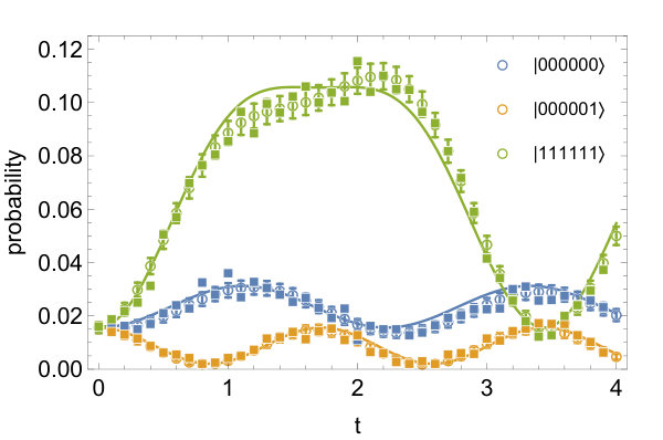 Figure 1
Peer Reviews
No public reviews on file for this paper yet. If you reviewed it on a platform where reviews are public (OpenReview, ICLR, NeurIPS, ICML), you can paste yours below so the community can read it here.
Videos
No videos yet. Explain this paper in a talk, walkthrough, or lecture? Add one.
NuQS Collaboration
Sigma models on quantum computers
Andrei Alexandru
Department of Physics, The George Washington University, Washington, D.C. 20052, USA
Department of Physics, University of Maryland, College Park, MD 20742, USA
Paulo F. Bedaque
Department of Physics, University of Maryland, College Park, MD 20742, USA
Henry Lamm
Department of Physics, University of Maryland, College Park, MD 20742, USA
Scott Lawrence
Department of Physics, University of Maryland, College Park, MD 20742, USA
Abstract
We formulate a discretization of sigma models suitable for simulation by quantum computers. Space is substituted by a lattice, as usually done in lattice field theory, while the target space (a sphere) is replaced by the “fuzzy sphere”, a construction well known from non-commutative geometry. Contrary to more naive discretizations of the sphere, in this construction the exact symmetry is maintained, which suggests that the discretized model is in the same universality class as the continuum model. That would allow for continuum results to be obtained for very rough discretizations of the target space as long as the space discretization is made fine enough. The cost of performing time-evolution, measured as the number of CNOT operations necessary, is , where is the number of spatial sites, the maximum time extent and the time spacing.
I Introduction
The advent of quantum computers opens up a new method to attack several physics problems which have, up to now, remained intractable. Perhaps the most interesting of those is the numerical treatment of many-body/field theories theories with sign problems. In particular, the nonperturbative calculation of real time observables, where very little progress has been made up to now Berges et al. (2007); Alexandru et al. (2017); Berges and Stamatescu (2005), is an obvious target for quantum computation. Of course, the hope of attacking these problems hinges on being able to formulate quantum field theories in a way suitable for quantum computers. This topic is still in its infancy. The naive expectation is that fermionic fields can be more easily implemented in quantum computers as a qubit can encode the presence or absence of a fermion in a given state. This is born out by the few existing calculations that have been performed on quantum comptuers Martinez et al. (2016); Klco et al. (2018); Lamm and Lawrence (2018). Bosonic fields are not so simply implemented. The attempts made up to now involve either eliminating the bosonic fields using some special property of the model or truncating the occupation number at any given site Hackett et al. (2018); Macridin et al. (2018); Yeter-Aydeniz et al. (2018); Klco and Savage (2018); Bazavov et al. (2015); Zhang et al. (2018); Unmuth-Yockey (2018); Unmuth-Yockey et al. (2018); Zache et al. (2018); Raychowdhury and Stryker (2018); Kaplan and Stryker (2018); Stryker (2018). The situation is analogous to the early days of (classical) computing in field theory. Classical bits also seem more amenable at describing fermionic than bosonic fields as the cost of storing and manipulating reasonable approximations to real numbers was too high to be practical in the early days. There were at the time several attempts at substituting bosonic continuous field values by a finite set of values Lisboa and Michael (1982); Flyvbjerg (1984a, b); Bhanot and Rebbi (1981); Jacobs and Rebbi (1981). In all these schemes the symmetry of the model is reduced by the discretization of the bosonic fields.
When discretization reduces the symmetry it is unclear whether, in the spacetime continuum limit, the original model is recovered. For instance, the non-linear sigma model in one spatial dimension with fields taking values on a sphere was studied in the approximation where the sphere is substituted by the vertices of a platonic solid. It seems to still be controversial whether the dodecahedron model is in the same universality class as the original spherical model Hasenfratz and Niedermayer (2001a); Caracciolo et al. (2001a); Hasenfratz and Niedermayer (2001b); Patrascioiu and Seiler (1998); Krcmar et al. (2016); Caracciolo et al. (2001b). In the case of gauge theories the question, at least for abelian theories, was settled long ago: abelian gauge theories with any finite discrete group are not in the same universality class as the model and do not approach the gauge theory as the spacetime continuum limit is taken Ukawa et al. (1980); Creutz et al. (1979); Grosse and Kuhnelt (1981).
This suggests that, to obtain the right continuum limit, we should construct a scheme where all the symmetries of the original model are maintained while discretizing the field variables in order to make the Hilbert space to have finite (and hopefully small) dimension. The topic of this paper is to present such a formulation. It is based on a well known construction in non-commutative geometry (the “fuzzy sphere” Hoppe (1989); Madore (1992)) that has been used before in the study of (super)-membranes. The resulting system can be simulated on a quantum computer with two qubits per spatial site. We implement our simulation scheme on a simulated quantum computer and verify it produces the right results. The number of gates required is of the order of , where is the number of spatial sites, the maximum time extent and the time discretization step.
II Sigma model on the fuzzy sphere
The sigma-model is defined on a discretized space by the Hamiltonian
[TABLE]
where is a unit three-dimensional vector, is the Laplace-Beltrami operator on , and the sum runs over the spatial lattice sites. The global symmetry , where is an orthogonal matrix, is evident. This model is asymptotically free in one spatial dimension 198 (1987).
In the Hamiltonian formalism, the wave function is a function of copies of the sphere , . The Hilbert space is infinite dimensional even for . We will approximate this model by substituting the target space (the sphere) by the “fuzzy sphere” Hoppe (1989); Madore (1992). The fuzzy sphere is not defined as a subset of points of the sphere; instead, it is the functions on the sphere that are substituted by elements of a finite dimensional Hilbert space. Let us demonstrate the construction first in the case. The wave function of the system is a function of and can be expanded as
[TABLE]
with the constraint . In the fuzzy sphere regularization we substitute this Hilbert space by the space of matrices
[TABLE]
where , are generators of in a given representation (normalized such that ). The important difference between Eq. (2) and Eq. (3) is that the sum in Eq. (3) terminates (for instance, if , ). Thus the infinite dimensional Hilbert space of functions on the sphere is substituted by a space of dimension . Since the space is finite dimensional it can be informally thought of as being the space of functions defined on a space with a finite number of points, the fuzzy sphere. In the case, the space of matrices is four-dimensional and the fuzzy sphere can be informally thought of as a 4-point discretization of the sphere. However, the “points” of the fuzzy sphere are “spread out” and choosing them does not break rotation symmetry. Notice that the fuzzy sphere is not defined as a subset of points of the sphere. It is the algebra of functions on the sphere that is deformed into a (non-commutative) algebra given by matrix multiplication. Still, the fuzzy sphere is an approximation to the sphere in the sense that operation defined on the sphere can be approximated by equivalent constructions on the fuzzy sphere. For instance, the norm in the sphere and on the fuzzy sphere satisfy:
[TABLE]
We refer to the references Madore (1992) for a discussion of the standard geometrical constructs of the sphere framed in terms of the algebra of functions (and their extensions to the fuzzy sphere). In particular, the Hamiltonian of the sigma model with one spatial site is simply the Laplacian on the sphere. (This describes the quantum mechanics of a free particle on the sphere.)
[TABLE]
with a normalization factor. The eigenvalues of the Laplacian operator on the sphere are for with mulitplicities . When the spectrum of its fuzzy version is exactly the same but truncated to its lowest values. This is in contrast to other discretizations of the sphere where the lowest eigenvalues are reproduced only approximately. Notice also that, as stressed before and contrary to other discretizations of the sphere, the fuzzy Laplacian has an exact invariance , where is the representation of the rotation .
From now on we will work with so the dimension of the Hilbert space at each site is 4. A convenient basis for this space is: and which satisfies . In a system with spatial sites, the Hilbert space of the system is the tensor product of single-site Hilbert spaces. The generic wavefunction can be written as
[TABLE]
The kinetic term of the Hamiltonian is the sum of Eq. (5) acting on the Hilbert space of each site and it is diagonal in the basis (for a single site operator , denotes the operator acting on site .) In the basis the kinetic term is represented by a sum of similar tensor products of matrices with
[TABLE]
The eigenvalues of are then , with , that is, the kinetic energy of site is 0 if or otherwise.
The “interaction” term arises from expanding the nearest-neighbor interaction term in Eq. (1): with . They involve only two neighbor sites at a time (one link). In the basis the operators are represented by the following matrices :
[TABLE]
where is the two-dimensional identity matrix and ’s are Pauli matrices. The interaction term in the basis is the matrix . By this we mean that the element is where and are the numbers that have the representation in basis 4 and respectively (the matrix indices run from [math] to .)
III Implementation of time evolution and estimate of resources
The implementation of the time evolution of the model in terms of quantum gates starts by splitting the time evolution over a number of smaller steps and each time step using the Suzuki-Trotter formula. Each time step is further split into the evolution due to the four parts of :
[TABLE]
The state of the system is time-evolved by first applying the kinetic term site-by-site; the site order does not matter since the for different commute. We follow the kinetic term with the first interaction term . This evolution is done link-by-link, and again, the order does not matter, as all commute with each other. We use periodic boundary conditions, so the evolution of the link from to is followed by evolution of a link from to . The link-by-link evolution is repeated for and . This completes one time step of the total time evolution. The whole process is then repeated times.
The local four-dimensional Hilbert space is encoded by two qubits so
[TABLE]
with the pair of qubits (for instance, ) being the binary digits of the value of the corresponding index . For instance, corresponds to and corresponds to . In this basis, the kinetic term evolution at each site corresponds to the matrix
[TABLE]
where from now on we set and for simplicity. The circuit implementing the kinetic term evolution is depicted on the left of Fig. (1). Since the interacting term is related by a similarity transformation to , with the change of basis given by single qubit operations (here is the Hadamard and the phase one-qubit gates.) Similarly, since , and are related to , via similarity transformations involving only single qubit operations. We now use the fact that a controlled-NOT (CNOT) gate implements a similarity transformation that takes into and that is simply a rotation on the left qubit. For we apply this for and qubit pair, whereas for the other two terms we have to apply the CNOT transformation on the and pairs to reduce to , and then a CNOT tranformation on the pair to reduce the exponentiation to a single qubit rotation. The quantum circuits implementing these operations are depicted in Fig. (1).
The counting of quantum gates is, of course, dependent on the instruction set available on the hardware. However, the difficulty in the hardware implementation of two-qubit gates makes it unlikely that any two-qubit gate besides the CNOT gate will be available in hardware. CNOT gates are also, by far, the ones likely to generate decoherence. Thus, we will only count the number of CNOT gates required in our implementation. The kinetic term circuit has 2 CNOT gates per site (notice that a controlled- operation requires two CNOT gates to be implemented in usual architectures). The and link terms seems to require CNOT gates per site. However, since we apply on every link the gates shown in the dashed box in Fig. (1) cancel between adjacent links and do not have to be applied. The result is that only CNOT gates per link are required. A similar thing happens to the links. Finally, requires CNOT gates, for a total of 12 CNOT gates per site (for periodic boundary conditions, where there are as many links as sites). Since steps are needed for a total time evolution , CNOT gates are required to implement in our three-site model. This gate depth renders the model inaccessible to the current generation of processors. As a proof-of-principle, however, we run our algorithm in a quantum computer simulator (QISKIT Santos (2017); Cross et al. (2017)) for and the results are shown in Fig. (2). The results in the figure were obtained with and show, for illustrative purposes, the probabilities of finding, as a function of time step, the states and starting with the initial state with equal amplitudes of all elements of the basis obtained by applying a Hadamard transformation on the state . In the same figure we show the exact time evolution and “Trotterized” evolution by multiplying the appropriate matrices. The error bars reflect the expected variance from quantum mechanical measurement.
It is important to stress that every step in our construction can be easily can be carried out in much bigger lattices and even in more spatial dimensions. The size of the blocks of time evolution – involving at most 4 qubits at a time – are independent of the system size. Also, the time evolution due to the kinetic term can be applied simultaneously to all sites and the evolution due to the hopping term can be applied simultaneously to half of the links at once. The method is essentially unchanged as the number of spatial dimensions is increased. Unfortunately, in the implementation in terms of quantum circuits we found, the number of CNOT gates is a little too large for current quantum computers available to us. Our attempts at running it on the IBM’s ibmqx4 machine resulted in mostly noise.
IV Conclusions and Prospects
One of the issues to be faced on the road to using quantum computers in quantum field theory is the presence of bosonic fields. The Hilbert space of a bosonic theory has an infinite number of dimensions per spatial site, while that for a fermionic theory is finite dimensional. On the other hand, the Hilbert space describing a quantum computer with a finite number of registers is finite dimensional. Thus, even after discretizing space, some further truncation of the field space will be required Hackett et al. (2018); Klco et al. (2018). We propose a method to accomplish this while, at the same time, preserving the symmetry of the theory.
There are two ways in which our fuzzy sphere model approximates the continuum sigma model. First of all, by increasing the dimension of the representation of the fuzzy sphere approaches the sigma model defined by Eq. (1). Perhaps more interesting is the fact that the fuzzy model, defined by (generalized to a large number of spatial sites), and the sigma model defined by the lattice hamiltonian Eq. (1), are likely to approach the same continuum limit as . In fact, the continuum limit of the sigma model is obtained by tuning and is such a way as to keep physical quantities (mass gap, scattering amplitudes) fixed in physical units (perturbation theory indicates that the model is asymptotically free so the correct scaling is 198 (1987)). In this limit, details of the Hamiltonian become irrelevant and any other Hamiltonian with the same field content and symmetries, on account of universality, give rise to the same continuum limit Zinn-Justin (2002). More precisely, any other operators, consistent with the symmetry, is of higher dimension and, presumably, irrelevant in the continuum limit. The reasonable assumption of universality can be checked in a classical calculation. The “Trotterized” time evolution operator (Eq. (9)) corresponds to an action discretized in both time and space. A Monte Carlo calculation using this action (analytically continued to imaginary time) can demonstrate whether the fuzzy model is indeed in the same universality class as the sigma model and has, therefore, the same limit.
Among theories of physical significance, bosonic fields also appear in principal chiral models (as, for instance, in low energy QCD) and gauge theories. These bosonic fields take values on group manifolds. A slight modification of the scheme proposed in the present paper can also be used in these cases, but it is somewhat more involved. A full account of these extensions will appear separately.
Acknowledgements.
A.A. is supported in part by the National Science Foundation CAREER grant PHY-1151648 and by U.S. Department of Energy grant DE-FG02-95ER40907. A.A. gratefully acknowledges the hospitality of the Physics Departments at the Universities of Maryland where part of this work was carried out. P.B., S.L., and H.L. are supported by the U.S. Department of Energy under Contract No. DE-FG02-93ER-40762. The authors are grateful to Zohreh Davoudi for conversations on quantum computing, and to Jesse Stryker for helpful comments.
The reference list from the paper itself. Each links out to its DOI / PubMed record.
- 1Berges et al. (2007) J. Berges, S. Borsanyi, D. Sexty, and I. O. Stamatescu, Phys. Rev. D 75 , 045007 (2007) , ar Xiv:hep-lat/0609058 [hep-lat] . · doi ↗
- 2Alexandru et al. (2017) A. Alexandru, G. Basar, P. F. Bedaque, and G. W. Ridgway, Phys. Rev. D 95 , 114501 (2017) , ar Xiv:1704.06404 [hep-lat] . · doi ↗
- 3Berges and Stamatescu (2005) J. Berges and I. O. Stamatescu, Phys. Rev. Lett. 95 , 202003 (2005) , ar Xiv:hep-lat/0508030 [hep-lat] . · doi ↗
- 4Martinez et al. (2016) E. A. Martinez et al. , Nature 534 , 516 (2016) , ar Xiv:1605.04570 [quant-ph] . · doi ↗
- 5Klco et al. (2018) N. Klco, E. F. Dumitrescu, A. J. Mc Caskey, T. D. Morris, R. C. Pooser, M. Sanz, E. Solano, P. Lougovski, and M. J. Savage, Phys. Rev. A 98 , 032331 (2018) , ar Xiv:1803.03326 [quant-ph] . · doi ↗
- 6Lamm and Lawrence (2018) H. Lamm and S. Lawrence, Phys. Rev. Lett. 121 , 170501 (2018) , ar Xiv:1806.06649 [quant-ph] . · doi ↗
- 7Hackett et al. (2018) D. C. Hackett, K. Howe, C. Hughes, W. Jay, E. T. Neil, and J. N. Simone, (2018), ar Xiv:1811.03629 [quant-ph] .
- 8Macridin et al. (2018) A. Macridin, P. Spentzouris, J. Amundson, and R. Harnik, Phys. Rev. Lett. 121 , 110504 (2018) , ar Xiv:1802.07347 [quant-ph] . · doi ↗