A central limit theorem for integrals of random waves
Matthew de Courcy-Ireland, Marius Lemm

TL;DR
This paper establishes a central limit theorem for the mean-square of high-frequency random waves on compact Riemannian manifolds, utilizing advanced integral estimates and the local Weyl law.
Contribution
It introduces a universal CLT for random waves on any compact Riemannian manifold, extending previous results to arbitrary dimensions and shrinking sets.
Findings
Proves a CLT for the mean-square of random waves in high-frequency limit.
Uses a novel estimate involving Bessel functions and Gegenbauer's addition formula.
Demonstrates universality across different manifold geometries.
Abstract
We derive a central limit theorem for the mean-square of random waves in the high-frequency limit over shrinking sets. Our proof applies to any compact Riemannian manifold of arbitrary dimension, thanks to the universality of the local Weyl law. The key technical step is an estimate capturing some cancellation in a triple integral of Bessel functions, which we achieve using Gegenbauer's addition formula.
Click any figure to enlarge with its caption.
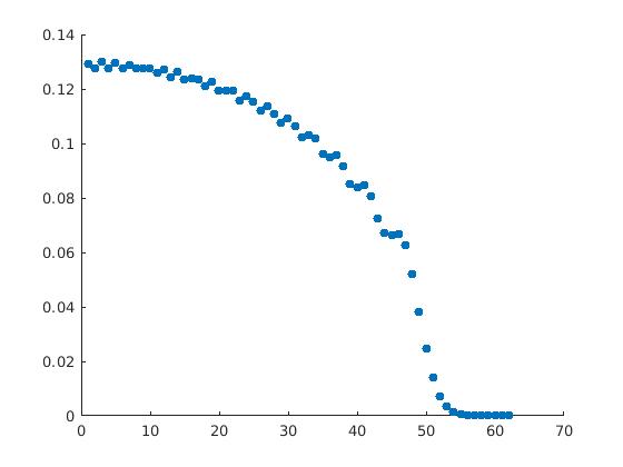 Figure 1
Peer Reviews
No public reviews on file for this paper yet. If you reviewed it on a platform where reviews are public (OpenReview, ICLR, NeurIPS, ICML), you can paste yours below so the community can read it here.
Videos
No videos yet. Explain this paper in a talk, walkthrough, or lecture? Add one.
Taxonomy
TopicsGeometry and complex manifolds · Geometric Analysis and Curvature Flows
A central limit theorem for integrals of random waves
Matthew de Courcy-Ireland
Department of Mathematics
Princeton University
Princeton NJ 08544 and Institute of Mathematics, EPFL, Lausanne CH-1015
and
Marius Lemm
School of Mathematics
Institute for Advanced Study
Princeton NJ 08540
and Department of Mathematics
Harvard University
Cambridge MA 02138
(Date: March 14, 2019)
Abstract.
We derive a central limit theorem for the mean-square of random waves in the high-frequency limit over shrinking sets. Our proof applies to any compact Riemannian manifold of arbitrary dimension, thanks to the universality of the local Weyl law. The key technical step is an estimate capturing some cancellation in a triple integral of Bessel functions, which we achieve using Gegenbauer’s addition formula.
1. Introduction
The goal of this paper is to prove a central limit theorem for , where is a random wave and the ball may shrink with the wavelength of . On any compact manifold with a Riemannian metric and corresponding Laplace operator , the random functions we have in mind are given by
[TABLE]
where the eigenfunctions solve with eigenvalues in a window . The coefficients are independent Gaussians of mean 0 and identical variance. The choice of variance will disappear when we pass to the standardized random variable
[TABLE]
which is invariant under scaling by a constant multiple or, what is the same, scaling the variance of the coefficients. Nevertheless, it is natural to choose the variance of each coefficient inversely proportional to the number of terms in the sum (1.1), so that . A standard Gaussian has characteristic function
[TABLE]
and our main result is an estimate comparing to this.
Theorem 1.1**.**
For any compact Riemannian manifold of dimension , any window with bounded above, and a geodesic ball shrinking at such a rate that and , we have convergence of characteristic functions
[TABLE]
for any fixed parameter .
The characteristic function \mathbb{E}\big{[}e^{itZ}\big{]} is defined for all real and, once is sufficiently large, for any fixed complex . In particular, Theorem 1.1 implies convergence in distribution.
Corollary 1.2**.**
(Central Limit Theorem) In the limit that with , as above, the standardized mean squares converge in distribution to a Gaussian of mean 0 and variance 1:
[TABLE]
For example, one could take and for a sufficiently small . It is important for our proof that , although one might expect the Central Limit Theorem to apply also for sufficiently small fixed radii in the limit . The scale is significant because it is the natural wavelength for Laplace eigenfunctions of frequency , and hence for the random waves (1.1). We assume that so that a length scale is enough to contain many oscillations of , and we have in mind that arbitrarily slowly so that one is almost at the wave scale. We do not expect the central limit theorem to hold if remains bounded, as we explain in Section 10.3, so that the wave scale provides a natural barrier.
We now give an overview of our strategy for proving Theorem 1.1 and some of the notation we will employ. Throughout the paper, we write as an abbreviation for sums over a given window of frequencies . For example, we have already done so in (1.1). We use the notations
[TABLE]
with the same meaning: there is a constant such that for all sufficiently large values of the variable(s) . We write if both of the approximate inequalities and hold, that is, there are constants such that
[TABLE]
If the constants depend on parameters, we indicate this with subscripts, as in
[TABLE]
The function is not necessarily real when we write , but we only write when both functions are positive. In Section 2, we compute the characteristic function of a quadratic form in Gaussian random variables, which includes as a special case. We give a sufficient condition for such a quadratic form to obey the Central Limit Theorem.
Proposition 1.3**.**
Given a sequence of symmetric, positive definite matrices and standard Gaussian vectors , let be the standardized quadratic form
[TABLE]
If
[TABLE]
as , then the characteristic function of obeys
[TABLE]
This can be seen as an instance of Lyapunov’s criterion for deriving a central limit theorem [5, p.362]: If is a sum of independent random variables, perhaps not with the same distribution, and is small compared to for some , then converges to a Gaussian as . Proposition 1.3 takes , and one diagonalizes the quadratic form to obtain a sum of independent random variables. For a quadratic form in Gaussians, one can replace the general argument of Lyapunov’s criterion with an explicit computation of the characteristic function.
In the case of , the matrix has a special form that allows the traces to be computed in terms of the two-point function
[TABLE]
We have so that, after choosing the variance of the coefficients, gives the correlations between values of at different points. In Section 3, we reformulate the criterion of Proposition 1.3 as
Proposition 1.4**.**
If is a Gaussian random function with two-point function satisfying
[TABLE]
as the ball shrinks, then the local integral obeys the Central Limit Theorem in the form
[TABLE]
Theorem 1.1 is then deduced from the following two estimates:
Theorem 1.5**.**
In any dimension ,
[TABLE]
Theorem 1.6**.**
In dimensions ,
[TABLE]
In Section 4, we use the local Weyl law to approximate and it is for this purpose that Theorem 1.1 assumes . In Section 5, we prove Theorem 1.5, and in particular give a lower bound on the denominator , which is essentially the variance of . In Section 6, the hypothesis comes into play as we approximate the triple integral in the numerator by a Euclidean version. For , we bound this integral from above in Sections 7 and 8, completing the proof of Theorem 1.6 in Section 9 for dimensions . We prove the two-dimensional case of Theorem 1.1 in Section 10.2 by a different argument: reducing to the case where is the round sphere.
For context, we recall Berry’s Random Wave Model [4], which uses monochromatic random waves of the form (1.1) as a stand-in to make predictions about non-random eigenfunctions. This is expected to be a good approximation for chaotic systems. The model applies to high-frequency Laplace eigenfunctions on a manifold of negative curvature and suggests that, at an appropriate scale, they should be uniformly distributed. Related to this is the Quantum Unique Ergodicity conjecture of Rudnick and Sarnak [24] that on a negatively curved manifold ,
[TABLE]
for any fixed measurable subset of and any sequence of Laplace eigenfunctions with growing eigenvalue . This is one of our motivations for considering local integrals , and the limit corresponds to the expected value of when is taken at random. The eigenvalue equation imparts a quantum interpretation, being the probability density of a single quantum particle in .
The quantum ergodicity theorem proved by Shnirelman [25, 26], Colin de Verdière [9], and Zelditch [29] shows that negative curvature implies convergence along a full subsequence of eigenfunctions, or equivalently on average over the eigenfunctions, but allows many other subsequential limits besides the uniform measure. Although it remains unknown whether the uniform measure is the only possibility, work of Anantharaman [1], Anantharaman-Nonnenmacher [2], Anantharaman-Silberman [7], and Dyatlov-Jin [12] places significant constraints on the measures that arise as quantum limits in general. In examples of arithmetic origin, QUE has been proved in work of Lindenstrauss [20, 21], and Bourgain-Lindenstrauss [6], Jakobson [19], Holowinsky [18], Holowinsky-Soundararajan [17].
The deterministic problem being so difficult, it is of interest to randomize the function and study the fluctuations in . Our main result shows that for shrinking at a certain rate, one can expect central limit statistics.
The central limit theorem controls deviations of size in the sense that
[TABLE]
for any fixed . We also obtain the following concentration estimate at other scales.
Theorem 1.7**.**
If is sufficiently small in terms of the implicit constants in the previous theorems, then
[TABLE]
where is a numerical constant and as above. In particular, the conclusion holds if as .
Han and Tacy proved deviation bounds in a related setting in equations (4.4), (4.5) of [15], which was a motivation for the present work.
2. Characteristic function of a quadratic form in Gaussians
In this section, we prove Proposition 1.3. Our quantity of interest is a quadratic form in the random Gaussian coefficients , and therefore has an explicit characteristic function. Indeed, expanding the square in shows that
[TABLE]
Write , where is a centered Gaussian of unit variance and denotes the common variance among all . Writing for the vector with entries , we have
[TABLE]
where the matrix has entries
[TABLE]
The moment generating function can be computed explicitly by diagonalizing this symmetric matrix . Write , so that
[TABLE]
where are the eigenvalues of . For an orthogonal matrix and a standard Gaussian vector , the vector also has a standard Gaussian distribution. For small enough that for all , independence of the random variables implies that
[TABLE]
which is a product of Gaussian integrals. These can be evaluated as
[TABLE]
We summarize this as
Proposition 2.1**.**
If is a symmetric matrix with eigenvalues , then the moment generating function of the quadratic form in Gaussian random variables is
[TABLE]
where both sides are defined for sufficiently small that , being the largest eigenvalue of .
Note that, by differentiating the moment generating function,
[TABLE]
Indeed, let and differentiate with respect to starting from
[TABLE]
to
[TABLE]
and then to
[TABLE]
Taking gives and then . Thus, as claimed,
[TABLE]
Passing to the standardized random variable , write
[TABLE]
so that
[TABLE]
Taking logarithms,
[TABLE]
Expanding the logarithm , the linear term cancels:
[TABLE]
Now we take and standardize. Shifting and scaling and starting from
[TABLE]
we find that the characteristic function of the standardized quantity
[TABLE]
is
[TABLE]
The factor is the characteristic function of a standard Gaussian. To show that converges to a Gaussian, we will estimate the traces and show that they are negligible compared to .
We complete the proof of Proposition 1.3 by using the third moment to bound the higher ones. Since -norms are monotone, we have an upper bound
[TABLE]
Therefore, summing a geometric series,
[TABLE]
where the series converges for any fixed as long as
[TABLE]
Here, as in the rest of the paper, we write to denote inequality up to a constant, and refers to limits where as described in the Introduction. Thus an upper bound on the third moment and a lower bound on the second are enough to control all others. Combining this with (2.6), we obtain the following estimate for the characteristic function, as stated in the Introduction.
Proposition 1.3.
Given a sequence of symmetric, positive definite matrices , let be the standardized quadratic form
[TABLE]
If
[TABLE]
then the characteristic function obeys
[TABLE]
The rest of our work is to bound the second and third moments.
3. Moments and the two-point function
We now show how Proposition 1.4 is a special case of Proposition 1.3. For any quadratic form and any , we have
[TABLE]
but for the particular one , we can express the traces in terms of the kernel
[TABLE]
The matrix entries are . By writing the product of integrals over as a single integral over , we obtain
[TABLE]
When we take the (finite) sum under the integral, it factors into copies of the two-point function:
[TABLE]
With the extra factor of from the entries , the trace becomes
[TABLE]
In particular,
[TABLE]
We summarize this discussion in the following restatement of Proposition 1.4, which may be helpful in other examples besides the monochromatic ensemble.
Proposition 3.1**.**
If is a Gaussian random function with two-point function satisfying
[TABLE]
as the ball shrinks, then the local integral obeys the Central Limit Theorem.
In our example, we will use semiclassics to estimate and verify the assumption that this ratio of integrals tends to 0 as . The lower bound on the denominator is provided by
Theorem 1.5.
[TABLE]
while the upper bound on the numerator is
Theorem 1.6.
[TABLE]
4. Weyl’s law
The local Weyl law is an estimate for showing that it resembles a Bessel function at the scale . Such results were obtained by Hörmander in the regime , but we are interested in distances shrinking arbitrarily slowly as . In this situation, we have the following by work of Canzani and Hanin.
Theorem 4.1**.**
(Canzani-Hanin) Let be a compact manifold of dimension , with smooth Riemannian metric and corresponding Laplace eigenfunctions obeying . Fix any point . For a large parameter , let where arbitrarily slowly as . Then the spectral function
[TABLE]
can be written
[TABLE]
where the remainder satisfies
[TABLE]
Hörmander had already proved this with a remainder at most for of order . In Theorem 2 from [8], Canzani and Hanin improved this in two ways: allowing to shrink more slowly than and, assuming is not self-focal, achieving an error term instead of . Without the assumption on , their proof still gives for shrinking arbitrarily slowly, as we proceed to sketch. Proposition 18 in [8] is the main technical estimate, and it allows to be self-focal. The role of the non-self-focal assumption is to guarantee the estimate (43) in [8], which says roughly that there is a constant such that when , the remainder is at most for any . Without the (non)focal assumption, one still knows by Hörmander’s work that the remainder is on the diagonal and the same arguments from [8] (in particular Propositions 10 and 11) imply that remains for distances shrinking arbitrarily slowly.
The phase is an important aspect of [8]. It is defined as long as is less than the injectivity radius of , that is, even for distances of order 1. In contrast, Hörmander’s “adapted” phase functions are obtained from the eikonal equation, a differential equation which is not guaranteed to have solutions when is unbounded.
For a window of frequencies , the kernel is
[TABLE]
The remainders and are both . Therefore Theorem 4.1 (Theorem 2 from [8]) implies an estimate for . Canzani-Hanin state the result as Theorem 3 in [8], but again they are interested in obtaining an improved remainder in the most crisp regime under the assumption that are close to a non-self-focal point . In the present article, we avoid making this assumption at the price of taking a slowly growing window . Rescaling the integral for by , we have
[TABLE]
where we have suppressed the subscripts with the understanding that and are taken with respect to the metric at . With the multiplicative factor ,
[TABLE]
It follows that
[TABLE]
We assume , so the integration over the thin annulus can be appproximated by an integral over the sphere times the width . In polar coordinates at , is the identity matrix. Identifying and with the vectors in representing them in coordinates,
[TABLE]
Finally, the Bessel function appears because of the integral formula
[TABLE]
We summarize this as follows, writing for the distance between and .
Proposition 4.2**.**
For any compact manifold and radius as , the two-point function for is given approximately by
[TABLE]
where is the number of frequencies in the interval . We have
[TABLE]
for a positive constant depending only on the dimension.
We will often use Proposition 4.2 as an upper bound. The Bessel term is bounded, so we always have . This can be improved when is larger than since decays as :
[TABLE]
To explain the normalization in Proposition 4.2, we review the local and global versions of Weyl’s law. Weyl’s law for counting eigenvalues can be deduced from the local version by integrating on the diagonal . Indeed, for orthogonal eigenfunctions , we have
[TABLE]
This leads to the usual Weyl’s law that the number of eigenvalues in our window is
[TABLE]
where is the volume of the Euclidean unit ball in dimension . Recall that we write the Laplace eigenvalue as (largely to avoid confusion with the eigenvalues of , already called ). From the binomial expansion,
[TABLE]
If we choose or smaller, then and we can absorb the higher order terms into the error already present in Weyl’s law. We need to be larger than in order for the main term to dominate. Thus for diverging no faster than , we have
[TABLE]
The variance of the coefficients should be inversely proportional to this in order for to be normalized in (on average). Indeed, for orthonormal eigenfunctions , we have
[TABLE]
It is also of interest to study windows even larger than . In this case, the error from the binomial expansion overwhelms the error from Weyl’s law. If is proportional to instead of only , then there is no need to use the binomial formula and we instead have
[TABLE]
This is the case of band-limited random functions, synthesized from a band of frequencies between and .
5. Proof of Theorem 1.5
We have Weyl’s law
[TABLE]
and hence
[TABLE]
We write as a shorthand for the Bessel function
[TABLE]
We integrate over to get
[TABLE]
By the triangle inequality, the ball contains a ball with smaller radius and center shifted to , where . The integrand is nonnegative, so we have a lower bound by integrating only over the smaller ball. Shifting to polar coordinates with respect to , we have
[TABLE]
Indeed, the volume form in normal coordinates is given by
[TABLE]
since the volume form is obtained from the metric by and we have the expansion
[TABLE]
We have
[TABLE]
Again, we achieve a lower bound by integrating only over a subset , namely . For in this smaller ball, we have . Thus
[TABLE]
Change variables to in the inner integral, so that . Then
[TABLE]
We have . Also, the function is bounded because of the decay of -Bessel functions. It has a non-zero average value
[TABLE]
Hence
[TABLE]
In terms of , this means
[TABLE]
To have a main term, we must assume that
[TABLE]
We have
[TABLE]
so the condition is simply
[TABLE]
which is one of the assumptions in Theorem 1.1.
One can obtain a comparable upper bound by a similar argument. Although we only need a one-sided bound to compare and , it is worth knowing that the lower bound above is essentially of the correct order of magnitude. The ball is contained in the re-centered ball , so that
[TABLE]
As before, we shift to polar coordinates centered at . Weyl’s law gives a pointwise upper bound on :
[TABLE]
This diverges as , since we would be better off using the trivial bound for , but the singularity is integrable. We obtain
[TABLE]
Integrating over brings another factor of . The resulting upper bound for the integral is
[TABLE]
Under our assumption, is large compared to so that the terms involving or are even smaller than . Therefore the upper and lower bounds match up to a constant multiple:
[TABLE]
6. Euclidean integral for the third moment
We have stated our main theorem for any compact Riemannian manifold. This level of generality is possible because the radius of the ball is shrinking and the triple integral is therefore close to its Euclidean counterpart. Recall that we write and similarly for their approximations by Bessel functions. Write Weyl’s law in the form
[TABLE]
where is the Bessel function from (5.1). It follows that
[TABLE]
Write for Euclidean distance and for Riemannian distance between the points represented by and in coordinates. Because has bounded derivative,
[TABLE]
In a ball of radius , the relative error in approximating Riemannian distances by Euclidean ones is a factor of . Hence
[TABLE]
Let , , . We compare the integral to a Euclidean version, introducing a small error in order to pass to polar coordinates based at . Take polar coordinates where the radial coordinate ranges from 0 to . As in Section 5, the volume form is given approximately by its Euclidean counterpart, namely
[TABLE]
where the error depends on the curvature of . We integrate and conclude that
Proposition 6.1**.**
If is a ball of radius in a compact manifold with a smooth Riemannian metric, then
[TABLE]
where is a Euclidean ball of radius centered at the coordinates for the basepoint (or equally well, centered anywhere in since the Euclidean integral is translation-invariant).
For the original kernel , larger than by a factor of , this leads to an error . We assume so that this can be absorbed into the error term already with us from Weyl’s law. Thus we may proceed with the Euclidean integral.
Let us first see what upper bound follows from crude estimates ignoring cancellation in the Bessel integrand. In higher dimensions, the angular variables and range over instead of . With as the origin in Euclidean space, write
[TABLE]
Then
[TABLE]
We may choose the coordinates to make the north pole and then account for the integration over with an overall factor of . The distance ranges from 0 to . The distances and may be as large as , with an angular range starting from a full sphere for distances less than and shrinking to nothing as the distance approaches . More specifically, the condition is
[TABLE]
and similarly for with its angle . Thus the angles and obey
[TABLE]
and we may simply take the dot products and as the first coordinates and , if we commit to the north pole. Let us write for the range of defined by (6.2), and likewise for the range of .
The integral is, up to a factor ,
[TABLE]
where we write for the Bessel function. Change variables to , , , with change of measure
[TABLE]
The angles and are unaffected by this scaling. The integral becomes
[TABLE]
Think of the prefactor as , since is comparable to . We have
[TABLE]
which oscillates between values of order . Simply observing that
[TABLE]
and ignoring cancellation gives an upper bound
[TABLE]
The exponent must be improved to something larger than in order to beat the variance, since the denominator is .
7. Gegenbauer’s addition formula
To handle the term in the inner integral, we have recourse to
Fact 7.1**.**
(Gegenbauer’s addition formula, [22, formula 10.23.8], [28, p.362-368]) If , then for ,
[TABLE]
where are the Gegenbauer polynomials.
Recall that the polynomials are orthogonal over the interval with weight . Their maximum value is attained at
[TABLE]
The notation is shorthand for . Note that when the Gegenbauer polynomials are bounded by 1, no matter how high the degree. For our application, , so this bounded case arises when . In higher dimensions , at its largest grows as a power of . Nevertheless, the series in Fact 7.1 converges because of the rapid decay in as a function of .
To bring Gegenbauer’s addition formula to bear on our inner integral, note that
[TABLE]
so we may take . Write and for the region of integration over the angles and from (6.2), suppressing the dependence on the outermost variables and . The integral is
[TABLE]
Next we integrate over and . This can be interchanged with the sum over , again thanks to the rapid decay of as grows. This leaves us with
[TABLE]
For many ranges of the parameters, or is a full sphere , in which case is exactly 0 by orthogonality of the Gegenbauer polynomials. In general, we make the following claim.
Proposition 7.2**.**
For , , concentric arcs and as above, and degree
[TABLE]
Proof.
The angular ranges and are concentric spherical caps (centered at , the direction from to ). We may assume that , reversing the order of if need be. We integrate with respect to using polar coordinates based at . Thus assumes some interval of values depending on the distance between and , and also on the angle . Because , this interval contains since automatically lies in the range . The variable ranges over an interval where , or this interval together with if and exceed a hemisphere. This only changes by a sign and the argument below will apply equally well. Depending on the angle , lies somewhere between the extreme cases and . Note also that or else the hemispheres would merge. We write
[TABLE]
where is the volume element on and the polynomials are orthogonal on the interval with respect to the weight . For the integral over , note that with and ,
[TABLE]
We have the following exact antiderivative
[TABLE]
This is a special case of formula (18.17.1) in [22], which gives the integral of Jacobi polynomials:
[TABLE]
The conversion between the ultraspherical notation and the Jacobi polynomial is
[TABLE]
where denotes a rising factorial. We have
[TABLE]
Converting between and under the integral, as well as and outside it, therefore brings a factor
[TABLE]
as stated in (7.3).
For the definite integral, note that when , we have , so that only the upper endpoint contributes. It follows that
[TABLE]
We recall Szegő’s asymptotic formula (8.21.17) in [27]: For large degree , the Gegenbauer polynomial is given approximately by
[TABLE]
up to an additive error of , and even smaller if . In particular, applying this with in place of gives
[TABLE]
We have already noted that , and changing to corresponds to increasing by 2. Thus
[TABLE]
The large-argument bound then gives
[TABLE]
We have used the fact that to bound , the exponent being nonnegative. Taking account of the prefactor
[TABLE]
it follows that
[TABLE]
Integrating over and brings only a bounded factor (volumes of spheres, depending only on ) and the claim follows. ∎
Using Proposition 7.2, the upper bound for the third moment becomes
[TABLE]
8. Beginning, middle, and end
In this section, we estimate the following one-variable integral arising from Section 7.
Proposition 8.1**.**
As with ,
[TABLE]
whereas if , then
[TABLE]
for any , with a correspondingly small constant. Both cases (8.1) and (8.2) are uniform with respect to (or any bounded interval of ).
The proposition is easy to see for fixed , because the integrand is a bounded function of and the interval of integration has length at most . The difficulty lies in allowing to grow with , but we will see that the same reasoning applies after subdividing the integral depending on the size of . For our application, as before.
Fix a and let . Then split the integral as
[TABLE]
where the latter two ranges are empty if is large enough that . These ranges are chosen in light of the fact that is very small when is much less than , mildly decaying and oscillatory when is much larger than , and with a transition between these regimes taking place when . More precisely,
Proposition 8.2**.**
For and not necessarily an integer,
[TABLE]
For ,
[TABLE]
For any , but of particular importance when ,
[TABLE]
The first of these is inequality (10.14.15) in [22]. The latter two bounds are crude consequences of much more detailed asymptotics available for . See, for instance, (10.20.4) of [22] or Chapter 7.4 of [13] for statements. For proofs, see chapter 8 of Watson’s book [28] or Olver’s article [23]. Note that the bounds are compatible in the sense that (8.4) recovers (8.5) when is of order . Note also that (8.4) reduces to when is much larger than , for instance if is fixed.
In the initial range , we apply (8.3) with . First, we use
[TABLE]
to expand the upper bound
[TABLE]
as a power series in . Note the series expansion
[TABLE]
with for our application. It follows that
[TABLE]
In the range , we have . Thus
[TABLE]
Now we can use to bound the initial contribution by an elementary integral:
[TABLE]
for a constant .
For the middle contribution, we use the transitional bound together with for fixed to conclude that
[TABLE]
For the final contribution, we see from (8.4) that
[TABLE]
Changing variables to gives
[TABLE]
Because is integrable near and bounded for away from 1, we have
[TABLE]
If , then for any value of , only the initial segment is present and so the integral is exponentially small, as claimed in (8.2). If , then in principle there may also be contributions as large as and , both of which are dominated by for this range of . Thus the integral is of the order as claimed in (8.1). This proves Proposition 8.1.
9. Completing the proof
In Section 7, we used Gegenbauer’s addition formula to express the third moment as a sum obeying the upper bound
[TABLE]
up to a constant multiple. In Section 8, we estimated the integral appearing in the summands for each . In this section, we estimate the sum over and deduce that the third moment compares favourably to the variance. We write .
We distinguish a bulk contribution, where , from a tail contribution where . For in the bulk, combining the three ranges of integration gives the upper bound from (8.1):
[TABLE]
For in the tail, only the beginning of the integral is present:
[TABLE]
Since is summble, the tail contributes only a bounded amount in addition to the bulk sum:
[TABLE]
The upper bound on the third moment becomes
[TABLE]
This compares favourably to the variance:
[TABLE]
which converges to [math].
For any (positive definite) quadratic form in Gaussians, Proposition 1.3 gives
[TABLE]
We have shown that for our particular form in any dimension , the second and third moments obey
[TABLE]
This implies the central limit theorem in the form
[TABLE]
as . Thus we have proved the central limit theorem for using Gegenbauer’s addition formula.
10. Two-dimensional case
In dimension 2, we have so that Gegenbauer’s addition formula is not available and we must argue differently. Note that the variance bound is the same for as for higher , namely or just in this case. A significant difference is that the exponent on the weight becomes negative. The kernel decays only as instead of saving an additional power . The Gegenbauer polynomials reduce to Chebyshev polynomials .
As , the local Weyl law leads to the same triple integral in Section 6 no matter the global geometry of . As a result, if a direct calculation proves the limit theorem on any particular manifold, one can draw the same conclusion in general. Such a calculation is possible on the sphere, and we will deduce the two-dimensional case from the instance . First we review the theory of spherical harmonics, including the case of higher dimensions. In any dimension, one could in principle use the same strategy of reducing to the sphere, but the two-dimensional case is simplest.
Note that the window plays a minor role. Under the conditions of Theorem 1.1, the central limit theorem reduces to bounding the Euclidean multiple integrals and . These same integrals are obtained from the sphere with small enough that the window amounts to a single degree of spherical harmonics. Thus the general case of any manifold with a window as in Theorem 1.1 follows from the case of with, say, .
10.1. Spherical harmonics
The standard basis of spherical harmonics of degree on is parametrized by integers
[TABLE]
whose sum is the total degree . For any such vector together with a choice of sign , one has a spherical harmonic
[TABLE]
where denotes the Gegenbauer polynomial. As varies, these harmonics are orthonormal and span the space of all harmonics of degree . For real-valued harmonics, it suffices to replace by and (up to a factor of normalization). These functions come from separation of variables in the coordinates
[TABLE]
on , where the angles range from [math] to while the final angle ranges over a full circle . We refer to [13], section 11.2 and especially formula 11.2(23).
Fix any point of as origin, say . The distance to the origin is then given by . We separate variables into a radial part and an angular part varying over the lower-dimensional sphere . Thus
[TABLE]
where
[TABLE]
and the remaining factors are such that is a spherical harmonic of degree on . Note that
[TABLE]
and the corresponding coordinates on the lower-dimensional sphere are simply scaled by in order to get . The spherical volume element on is
[TABLE]
where is the spherical volume element on . In particular, two harmonics and with vectors are orthogonal on any ball because the angular parts are already orthogonal over . Note that the condition rules out the possibility that and agree on their angular coefficients but have . Such harmonics would be of different degree.
For the two-dimensional sphere , we have . The coordinates are just and . Because of the constraint , there is essentially just one component together with a choice of sign . Thus we have the usual basis harmonics
[TABLE]
Now expand any given harmonic in the basis functions with respect to a chosen origin:
[TABLE]
where varies over all vectors as above, that is, and the entries of are decreasing from to . We also specify a trigonometric factor via the choice of sign. By orthogonality, integrating over a ball around the origin gives a diagonal quadratic form in the coefficients :
[TABLE]
For our application, the functions must be normalized so that . Thus
[TABLE]
since the angular integrals over are the same whether we integrate over the ball of radius or over the whole sphere , that is, the ball of radius . Note that the radial part depends only on and . Given and , the extra components and the sign weight the corresponding summand by a combinatorial factor. For example, if , the weight is 2 because it must be that , leaving only the two choices of sign. Likewise, if , it must be that and the smaller components vanish, so the weight is again 2. But the larger the deficit between and the total degree , the more combinations arise. A simplification available for compared to higher-dimensional spheres is that are the only parameters and no further cases occur.
For large , we have Szegő’s asymptotic for the Gegenbauer polynomial:
[TABLE]
where . The error term is , and even smaller if . See formula (8.21.17) in [27]. For us, and . Thus
[TABLE]
10.2. Central limit theorem on the two-dimensional sphere
When , the Laplace eigenvalues are with multiplicity , where is the degree (instead of , as above in arbitrary dimension). If and is a small constant (for instance, ), then the window contains copies of a single frequency equal to . Note that , so we may take rather than as the key asymptotic parameter. The eigenvalues of the quadratic form are given by
[TABLE]
This was used in [10] to estimate the as follows. There are three cases, which we think of as “bulk”, “edge”, and “tail”.
Proposition 10.1**.**
Fix a point and choose for our basis functions the standard ultraspherical polynomials rotated so that is at the North pole . Then
[TABLE]
where the are independent standard Gaussians for and the coefficients satisfy
[TABLE]
for any and a ratio bounded away from . For close to , we have an upper bound
[TABLE]
For so large that , where , we have
[TABLE]
for a constant .
Thus the eigenvalues of follow the semi-circle law. Perhaps one should expect some GOE behaviour because is given by integrals and there is a large orthogonal group of symmetries acting by change of basis on the functions .
As in Section 2, to show that is approximately Gaussian, it is sufficient to show that for
[TABLE]
To verify (10.4), we can use the semicircle law from Proposition 10.1 to estimate . First, we bound the contributions from near or larger. Fix a value of and write as an abbreviation for . We have
[TABLE]
For larger , we have
[TABLE]
The tail sum is very small. For example, comparing to an integral gives
[TABLE]
with , so that , and . Meanwhile, the “bulk” contribution is
[TABLE]
For the main term, we have a Riemann sum approximation
[TABLE]
For the error term, we have
[TABLE]
Thus the bulk contribution is
[TABLE]
Compare this to the edge contribution, bounded by , and the tail contribution, which obeys the even stronger bound . For any chosen , these are negligible compared to the main term of order and even to the error term of order . Thus we have, for the sum over all three ranges,
[TABLE]
with an implicit constant proportional to . In particular,
[TABLE]
From this, we obtain
[TABLE]
which is negligible as provided . Even when we sum over all , we obtain a geometric series:
[TABLE]
A final detail remains: We took , which we now justify by using the semicircle law to show that the power series for does converge at that point. From the semicircle law Proposition 10.1, the largest are of order , whereas is of order . It follows that, for any given , once is sufficiently large we do have
[TABLE]
for all . The series will converge once is so large that
[TABLE]
Combining these estimates, we have
[TABLE]
and hence
[TABLE]
For any fixed , this converges to as , which completes our proof of Theorem 1.1.
10.3. Failure of the CLT at the wave scale
Suppose that for a fixed constant , or more generally that remains bounded as . At this scale, we do not expect the central limit theorem to hold, and a direct calculation on supports this. From the variance formula (3.1) with ,
[TABLE]
We have because they are the eigenvalues of the positive quadratic form . It follows that
[TABLE]
where is the eigenvalue corresponding to the zonal spherical harmonic. As in the proof of the semicircle law Proposition 10.1, we have
[TABLE]
But unlike Proposition 10.1, we now have of order 1, so that
[TABLE]
It follows that
[TABLE]
Thus the criterion of Proposition 1.3 fails, and we believe that instead of converging to a Gaussian, the standardized local integral converges to a weighted sum of finitely many squares of Gaussians (with a number of degrees of freedom proportional to , the higher values of being exponentially suppressed).
11. Tail probability
One consequence of Theorem 1.1 is that the random variable has tails satisfying
[TABLE]
for any fixed . Note that , and another approach is needed to control deviations where exceeds a given of larger size. One obtains such a bound using the foregoing estimates together with a Chernoff bound. Namely, for any for which is defined, the upper tail probability obeys
[TABLE]
The lower tail event can be treated with the same procedure applied to instead of . The parameter is at our disposal, and the optimal choice is to minimize . As we saw in Section 2,
[TABLE]
with both sides defined for , where is the largest . Differentiating with respect to , we find that the equation for the optimal is
[TABLE]
Upon expanding in a geometric series, the first term cancels and we obtain
[TABLE]
Truncating at suggests the choice
[TABLE]
but it is not clear whether , that is, whether this choice of is valid. Using our bound on the third moment we conclude that
[TABLE]
With the desired choice of ,
[TABLE]
by the third-moment bound for and the fact that is bounded above and below by constant multiples of . It follows that the choice (11.2) is valid provided
[TABLE]
or more generally when is a sufficiently small constant multiple of .
When is small enough that (11.2) is a valid choice of , the Chernoff bound gives
[TABLE]
assuming we can truncate the Taylor expansion at second order. This truncation is justified under the same condition allowing the choice of to begin with, since the higher terms can be bounded by This completes the proof of Theorem 1.7. ∎
Even when (11.2) is not valid, one can obtain an upper bound by choosing a different (and (11.2) is itself only an approximation to the optimal choice). The workaround from [11] is to instead take to be a small multiple of \big{(}\sum\lambda_{j}^{2}\big{)}^{-1/2}, the validity of which follows from the bound . This allows one to take, for example, of order 1 at the cost of replacing by in Theorem 1.7.
12. Conclusion and outlook
As explained in Section 5, the exponent in our lower bound on the variance is optimal. Less clear is the true size of the third moment. One approach to this would be to give an explicit treatment of higher-dimensional spheres along the lines of the semicircle law for .
One of the aspects of the Central Limit Theorem is its universality: The normal distribution appears as a limit for a wide class of underlying distributions for the coefficients. In contrast, we have assumed Gaussian coefficients from the beginning, so it is perhaps less surprising that one recovers a Gaussian in the limit. An interesting problem would be to prove the CLT for random waves with other distributions for the coefficients , not necessarily Gaussian. We expect that the central limit theorem will hold for a quite broad class of random coefficients. Indeed, it might not be necessary to randomize at all if the underlying manifold has favourable dynamical properties.
Some further examples of coefficients seem to be within reach, namely if (a) the vector of coefficients is rotation-invariant, or (b) several moments of the coefficient distribution agree with those of a Gaussian. Assuming (a), the vector of coefficients is rotation-invariant and as above one can diagonalize the quadratic form to obtain a sum of independent random variables. Lyapunov’s criterion then applies and reduces the central limit theorem to estimates for the second and third moments as above. Assuming (b) up to moments of order six, these estimates follow from the direct calculation with Gaussians carried out here. Note that the -th moment of the quadratic form only involves moments up to order of the coefficients of . For an example of rotation-invariant but non-Gaussian coefficients, one can take the vector of coefficients uniformly from the sphere . However, the coefficients in this example are not independent.
We have given an upper bound on the probability that deviates from its average, at least in some ranges. An interesting problem would be to use the theory of large deviations to give a comparable lower bound on this probability. It could also be possible to prove the Central Limit Theorem directly from this machinery.
Acknowledgments
We thank Yaiza Canzani for helpful discussions about Weyl’s law. MDCI thanks Peter Sarnak for his advice, encouragement, and support over the course of this work and thanks the Natural Sciences and Engineering Research Council of Canada for a PGS D grant. ML thanks Rupert L. Frank for multiple stimulating discussions on the topic, and thanks the Institute for Advanced Study for its hospitality during the 2017-2018 academic year.
The reference list from the paper itself. Each links out to its DOI / PubMed record.
- 1[1] N. Anantharaman, Entropy and the localization of eigenfunctions , Ann. of Math. (2), 168 (2008), 435–-475.
- 2[2] N. Anantharaman and S. Nonnenmacher, Half-delocalization of eigenfunctions for the Laplacian on an Anosov manifold , Ann. Inst. Four. (Grenoble), 57, 6 (2007), 2465–-2523.
- 3[3] N. Anantharaman and L. Silberman, A Haar component for quantum limits on locally symmetric spaces , Israel J. Math. v 195 no.1 493-447 (2013)
- 4[4] M. V. Berry, Regular and irregular semiclassical wave functions , J. Phys. A.: Math. Gen. 10 (1977) 2083-2091
- 5[5] P. Billingsley, Probability and Measure , 3rd ed. Wiley, New York, 1995
- 6[6] J. Bourgain and E. Lindenstrauss, Entropy of quantum limits , Comm. Math. Phys., 233 (2003), 153–-171.
- 7[7] M. Abramowitz and I. A. Stegun, Handbook of Mathematical Functions , National Bureau of Standards, Washington, D.C. (1972)
- 8[8] Y Canzani and B. Hanin, Scaling limit for the kernel of the spectral projector and remainder estimates in the pointwise Weyl law , Analysis & PDE, Vol. 8, No. 7 (2015), 1707-1732