Distribution of Brownian coincidences
Alexandre Krajenbrink, Bertrand Lacroix-A-Chez-Toine, Pierre Le, Doussal

TL;DR
This paper analyzes the probability distribution of total pairwise coincidence time among multiple independent Brownian particles, using advanced mathematical mappings to derive explicit formulas and asymptotic behaviors.
Contribution
It introduces a novel approach by mapping the coincidence time problem onto models like Lieb-Liniger, directed polymers, and KPZ, providing explicit formulas and asymptotics.
Findings
Derived closed-form probability distribution for coincidence time.
Obtained universal large deviation tail independent of geometry.
Validated analytical results with numerical simulations.
Abstract
We study the probability distribution, , of the coincidence time , i.e. the total local time of all pairwise coincidences of independent Brownian walkers. We consider in details two geometries: Brownian motions all starting from , and Brownian bridges. Using a Feynman-Kac representation for the moment generating function of this coincidence time, we map this problem onto some observables in three related models (i) the propagator of the Lieb Liniger model of quantum particles with pairwise delta function interactions (ii) the moments of the partition function of a directed polymer in a random medium (iii) the exponential moments of the solution of the Kardar-Parisi-Zhang equation. Using these mappings, we obtain closed formulae for the probability distribution of the coincidence time, its tails and some of its moments. Its asymptotics at large and small coincidence…
Click any figure to enlarge with its caption.
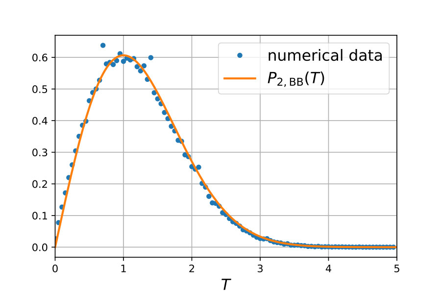 Figure 1
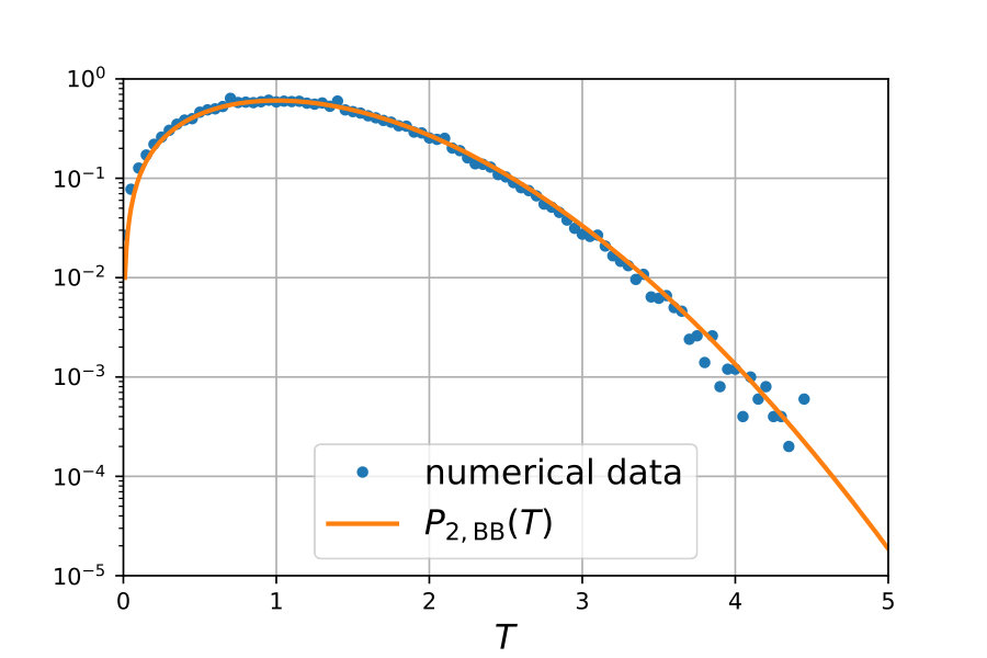 Figure 2
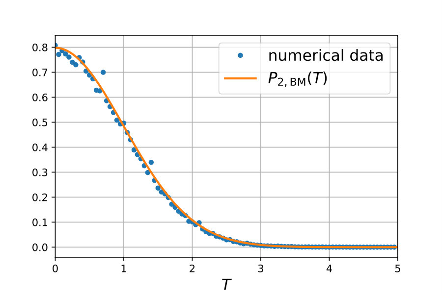 Figure 3
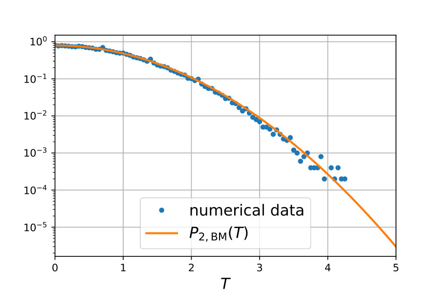 Figure 4
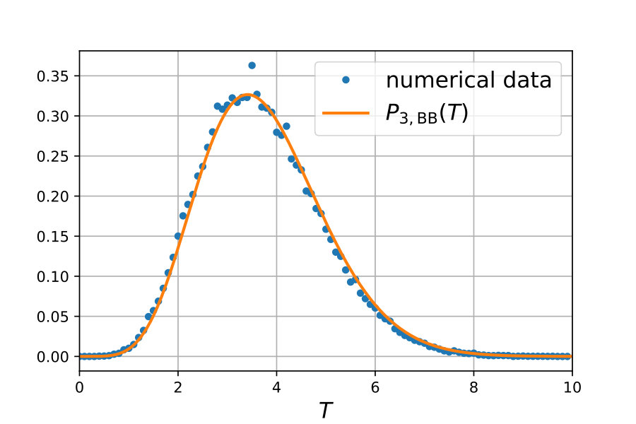 Figure 5
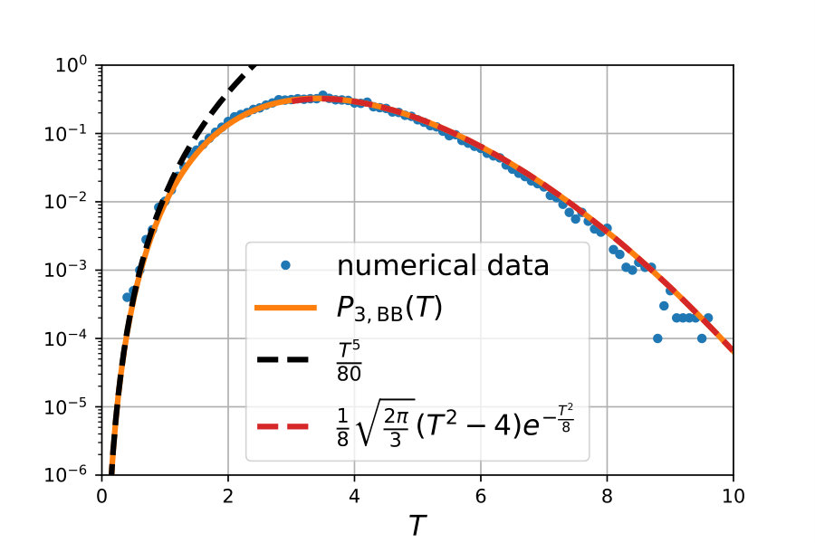 Figure 6
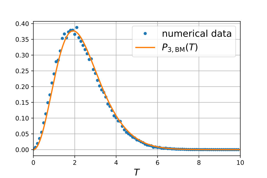 Figure 7
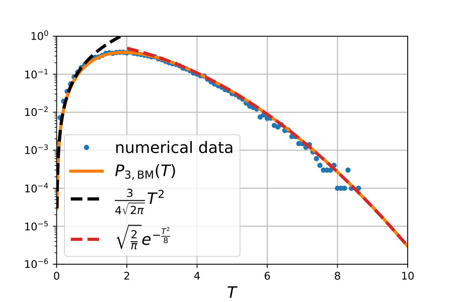 Figure 8
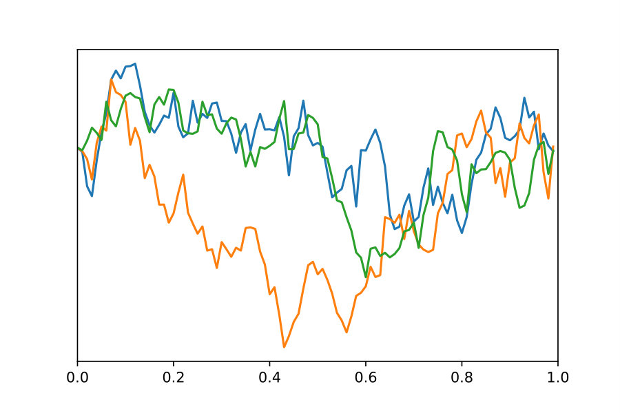 Figure 9
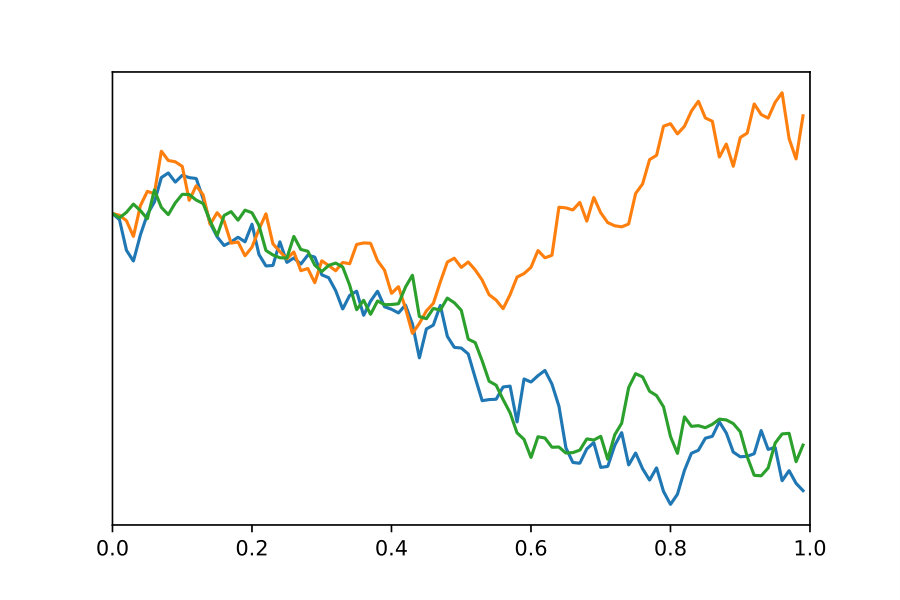 Figure 10
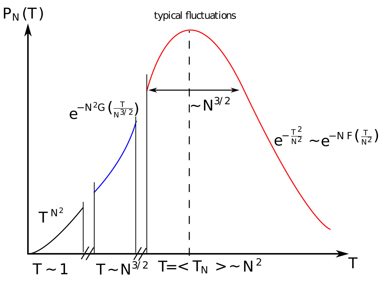 Figure 11
Peer Reviews
No public reviews on file for this paper yet. If you reviewed it on a platform where reviews are public (OpenReview, ICLR, NeurIPS, ICML), you can paste yours below so the community can read it here.
Videos
No videos yet. Explain this paper in a talk, walkthrough, or lecture? Add one.
Distribution of Brownian coincidences
Alexandre Krajenbrink
Laboratoire de Physique de l’Ecole Normale Supérieure,
PSL University, CNRS, Sorbonne Universités,
24 rue Lhomond, 75231 Paris Cedex 05, France
Bertrand Lacroix-A-Chez-Toine
LPTMS, CNRS, Univ. Paris-Sud, Université Paris-Saclay, 91405 Orsay, France
Pierre Le Doussal
Laboratoire de Physique de l’Ecole Normale Supérieure,
PSL University CNRS, Sorbonne Universités,
24 rue Lhomond, 75231 Paris Cedex 05, France
Abstract
We study the probability distribution, , of the coincidence time , i.e. the total local time of all pairwise coincidences of independent Brownian walkers. We consider in details two geometries: Brownian motions all starting from [math], and Brownian bridges. Using a Feynman-Kač representation for the moment generating function of this coincidence time, we map this problem onto some observables in three related models (i) the propagator of the Lieb Liniger model of quantum particles with pairwise delta function interactions (ii) the moments of the partition function of a directed polymer in a random medium (iii) the exponential moments of the solution of the Kardar-Parisi-Zhang equation. Using these mappings, we obtain closed formulae for the probability distribution of the coincidence time, its tails and some of its moments. Its asymptotics at large and small coincidence time are also obtained for arbitrary fixed endpoints. The universal large tail, is obtained, and is independent of the geometry. We investigate the large deviations in the limit of a large number of walkers through a Coulomb gas approach. Some of our analytical results are compared with numerical simulations.
Contents
-
2 Coincidence time for Brownian bridges and KPZ equation with droplet initial conditions
-
2.1 Bethe ansatz solution of the Lieb-Liniger model for droplet initial conditions
-
2.2 Probability Distribution Function of the coincidence time
-
2.3 Full distribution of the coincidence time for Brownian bridges
-
2.5 Mean and variance of the coincidence time for Brownian bridges
-
3 Coincidence time for Brownian motions and KPZ equation with flat initial condition
-
3.1 Bethe ansatz solution of the Lieb-Liniger model for half-flat initial conditions
-
3.2.1 Moment generating function and probability distribution function for
-
3.3 Probability Distribution Function of the coincidence time
-
3.5 Mean and variance of the coincidence time for Brownian motions
-
4.2 Small asymptotics of the PDF for any and for any fixed final points
-
4.3 Large asymptotics of the PDF for any and arbitrary final and initial points
-
A Expected value of the coincidence time for non identical diffusing particles
-
B Details of the calculations of the distribution for Brownian bridges
1 Introduction and main results
1.1 Introduction
In this article, we study independent and identical diffusive Brownian processes. We want to characterise in details the statistics of the time spent by identical diffusing particles in the vicinity of each other, which we call the coincidence time. This problem is relevant for instance to analyse reaction networks of the type
[TABLE]
Indeed, for chemical species to react, they first have to encounter each other and then overcome the potential barriers. This takes a finite amount of time and this coincidence time plays a crucial role in the kinetics of the reaction. The behaviour of this coincidence time is highly dependent on the spatial dimension, as it is clear that the higher the dimension, the harder it is for diffusing particles to encounter one another. We limit our study of this problem to the case of dimension , where the number of encounters is maximum. We model the identical diffusing particles via independent one dimensional Brownian motions on the time interval
[TABLE]
where below we choose units such that . We consider the case where the diffusing particles are emitted at from a single point-like source for . We define the total time spent by these particles in a close vicinity of length to each other as
[TABLE]
where is the Heaviside step-function. We are particularly interested in the limit where the length is small compared to all the other scales of the problem and therefore define in the limit ,
[TABLE]
We will refer to this observable as the coincidence time of diffusing particles, i.e. the amount of time that these independent particles spend crossing each other 111 for calculational convenience below, each pair appears twice in the sum in our definition (4). . Note however that does not have the dimension of a time, which is a usual property of the local time of a stochastic process [1, 2, 3]. Using the Brownian scaling, the process has a trivial rescaling to the time interval , and we obtain the equality
[TABLE]
We will see in the following that the -dependence is however highly non-trivial. The case can be solved quite easily by considering the process which is also a simple diffusive process of same diffusion coefficient ,
[TABLE]
The coincidence time of the two Brownian particles can be expressed in terms of the local time of the process defined as
[TABLE]
Setting , we obtain
[TABLE]
The joint PDF of the local time and the final position was obtained by Borodin et al. [2] and exploited by Pitman [3] and reads
[TABLE]
We set and remind that in our convention. Using now the identities together with , we obtain the joint PDF of the coincidence time and the final algebraic distance between the diffusive particles as
[TABLE]
However, as soon as , one cannot define independent processes for which our coincidence time is a simple observable.
Here we will study the Probability Distribution Function (PDF) of for two cases, Brownian motions and Brownian bridges. In the first case (Brownian motion) one defines the Moment Generating Function (MGF) , where denotes the expectation value with respect to the PDF of for given initial conditions . This MGF can be expressed in the Feynman-Kač framework as an -dimensional path integral
[TABLE]
where . In this expression we wrote the sum as to represent the coincidence as a delta interaction between each pair of Brownian motions. As the final point is arbitrary, we integrated here over all the possible realisations. This situation corresponds to the right panel in Fig. 1. In the second case (Brownian bridges) we define the MGF as the following expectation value with fixed initial and final positions
[TABLE]
where is the free propagator. This situation corresponds to the left panel in Fig. 1.
The function can be interpreted as the imaginary time -body propagator of the bosonic Lieb-Liniger Hamiltonian [4]
[TABLE]
We therefore see that this MGF, eq. (13), for non-interacting diffusing classical particles is mapped onto the propagator of a quantum problem of identical bosons with a contact interaction. This problem is also related to other well-studied models: the directed polymer in a random potential, equivalent to the Kardar-Parisi-Zhang (KPZ) stochastic growth equation. Indeed, consider an elastic polymer of length and fixed endpoints and , in a random potential . Its partition function reads
[TABLE]
One may then compute the -point correlation function of the partition function, averaged with respect to the random potential (denoted as ) and obtain
[TABLE]
Taking now as a Gaussian white noise of variance ,
[TABLE]
the replica average in Eq. (16) reduces to the Lieb-Liniger real time propagator in Eq. (12) [5, 6, 7] with the value of the parameter , and satisfies the same evolution equation (14)222The constraint in (12) originates from the Itô prescription in the (Feynman-Kač) stochastic heat equation satistied by , equivalently in the definition of the path integral. . The directed polymer partition function is also equal to the droplet solution of the KPZ equation, through a Cole-Hopf transformation,
[TABLE]
Both the directed polymer and the KPZ equation correspond to the choice , i.e. to the attractive Lieb-Liniger model.
The moments (16) of the directed polymer problem, which correspond to exponential moments for the KPZ height field, have been studied extensively recently and exact formulae have been obtained for the droplet solution at arbitrary time [7, 8, 9]. The MGF of our diffusion problem, for independent Brownian bridges, and negative value of the parameter is thus related to these moments as follows
[TABLE]
where is the free Brownian propagator (for ). Explicit expressions of these moments were derived from the Bethe ansatz. Note that all initial and final points here are set to [math].
In this paper, we obtain complementary exact formula for the MGF for positive value , i.e. for the Laplace transform of the coincidence time . We study in particular the case of independent Brownian bridges denoted , and the case of Brownian motions starting from the same point, , with free final points, denoted . We also use the formula (19) for negative to obtain the large asymptotics of the PDF of . For that particular asymptotic behavior we obtain some more results for arbitrary fixed final points, using a formula for . We now summarize our main results.
1.2 Summary of the main results
Brownian bridges We obtain an exact formula for the PDF of the rescaled coincidence time for Brownian bridges as
[TABLE]
For , we obtain explicit formulae for respectively in Eq. (42) and (46). For general , we extract the small and large asymptotic behaviours as
[TABLE]
where is the Barnes-G function, is the usual Gamma function, is the Hermite polynomial of degree and the exponential factors are
[TABLE]
We also obtain the mean coincidence time in Eq. (56) and the variance in Eq. (60).
Brownian motions We obtain an exact formula for the MGF of the rescaled coincidence time for Brownian motions (i.e. with free final points), which depend on the parity of . It is given in Eq. (3.2.2) for even values of and in Eq. (3.2.2) for odd values. For , we obtain explicit formulae for the PDF ,
[TABLE]
For arbitrary values of , we obtained the expression of the PDF as:
** odd**
[TABLE]
** even**
[TABLE]
We further extracted the small and large behaviours as
[TABLE]
where is given in Eq. (135). The coefficients and are the same as for the Brownian bridge in Eq. (22). We also obtain the mean coincidence time in Eq. (119) and the variance in Eq. (121).
Finally, we extended our study to Brownian walkers with arbitrary fixed endpoints. The small asymptotics of the PDF for arbitrary final points (all initial points being at [math]) is given in (133). The large asymptotics of the PDF for any choice of initial and final points is displayed in (4.3).
A trivial consequence of our work is the PDF of the coincidence time for Brownian walkers interacting pairwise via a delta interaction of strength (of any sign). It is given in terms of the PDF for non-interacting Brownian calculated here, simply as
[TABLE]
The remaining of the paper is organised as follows. Section 2, is dedicated to the results for the case of Brownian bridges. In subsection 2.1, we describe how the Bethe ansatz applied to the Lieb-Liniger model allows to obtain a formula for the MGF.In subsection 2.2, we derive the exact formula in Eq. (20) for the PDF of the coincidence time for arbitrary . In subsection 2.3, we analyse this formula for . In subsection 2.4, we derive the asymptotic behaviours for and for arbitrary . In subsection 2.5, we obtain the mean and variance for arbitrary . Finally, in subsection 2.6, we analyse the large limit via Coulomb gas techniques. In Section 3, we extend all previous results - except the Coulomb gas - to the Brownian motions in the same fashion and derive the exact PDF for arbitrary Brownian motions given in Eqs. (25) and (24). In Section 4, we study some properties of the coincidence time for Brownian with arbitrary fixed endpoints. We obtain the exact expression of its PDF for and , the small asymptotics for any and the large asymptotics for arbitrary initial and final points. The latter is obtained using the properties of the ground state of the Lieb-Liniger model.
2 Coincidence time for Brownian bridges and KPZ equation with droplet initial conditions
2.1 Bethe ansatz solution of the Lieb-Liniger model for droplet initial conditions
The Lieb-Liniger Hamiltonian in Eq. (14) is an exactly solvable model using the Bethe ansatz. Here we need only the symmetric eigenstates of , which in the repulsive case , are single particle states. The eigen-energies of this system defined on a circle of radius form, in the large limit, a continuum indexed by real momenta ’s such that
[TABLE]
where the denote the eigenstates of . The calculation is similar to the one in refs. [7, 8] except that we retain here for only the particle states. Consider the imaginary time propagator at coinciding endpoints
[TABLE]
We now use that and we arrive at the following Laplace transform for the PDF of the coincidence time for Brownian bridges
[TABLE]
where we have divided by the result at which coincides with the free propagator .
We note that there is an alternative formula for the moments of the directed polymer problem, which was derived using Macdonald processes [9, 10]. Using this formula we can write the MGF of Brownian bridges equivalently as
[TABLE]
Note that this formula is valid only for , otherwise the contours are different. Using the symmetrization identity
[TABLE]
one can show that this formula is in agreement with (32).
2.2 Probability Distribution Function of the coincidence time
In this section we obtain from Eq. (32) an expression for the PDF of the coincidence time for the Brownian bridges. First, we use the Cauchy identity
[TABLE]
We then introduce the auxiliary variables such that
[TABLE]
Replacing in Eq. (32), we are now able to compute the integrals over , yielding
[TABLE]
Inverting the Laplace transform of this expression, we obtain the PDF of the rescaled coincidence time as
[TABLE]
where is the Heaviside step function. We start by analysing the case of , where the PDF can be computed explicitly before considering the general behaviour for arbitrary values of . This formula (40) is the most compact general expression that we could find. We show in the next section that it can be used to derive explicitly the PDF for small values of .
2.3 Full distribution of the coincidence time for Brownian bridges
Distribution for . In the case of , we will see how to extract the full PDF from Eq. (40). Setting , we may compute exactly the determinant in the integrand, yielding
[TABLE]
The first term in the integrand vanishes when deriving with respect to . The PDF can then be derived in a few steps as
[TABLE]
The asymptotic behaviours of this PDF are simple to extract as
[TABLE]
In Fig. 2, we compare our analytical formula of Eq. (42) with the numerical simulations of Brownian bridges (see Appendix C for the details of the simulations), showing an excellent agreement.
Note that in the case , this result can be obtained directly from Eq. (10) by setting the final distance between the diffusive particles and ensuring the normalisation of the probability
[TABLE]
As noted previously this method cannot be generalised to larger values of , a contrario with our exact formula in Eq. (40).
Distribution for . Starting from , the distribution cannot be obtained from a simple rescaling of the local time of a single Brownian motion,and we need to use our results in Eq. (40) for the Brownian bridge. In the case of , the determinant appearing in the integrand can still be computed quite easily, yielding
[TABLE]
where we used the symmetry between the ’s. After some computations (See Appendix B for details), we finally obtain the PDF
[TABLE]
Its asymptotic behaviours read
[TABLE]
In Fig. 3, we compare the analytical formula of Eq. (46) with the numerical simulations of Brownian bridges (see Appendix C for the details of the simulations), showing an excellent agreement.
2.4 Asymptotic behaviours of for arbitrary
We now come back to the case of Brownian bridges and analyse the tails of the PDF of the rescaled coincidence time respectively for and .
2.4.1 Small limit of the Probability Distribution Function
To obtain the small limit of , it is convenient to consider the limit of , which is given in Eq. (32). The trajectories which contribute to a small coincidence time are repelled from each others. In the Lieb-Liniger picture, this is consistent with the repulsive case where the states are described as single particle states rather than bound state. Taking the large limit of Eq. (32), we obtain
[TABLE]
where is the Barnes function. We have used the Mehta integral formula e.g. (1.5)-(1.6) in [11]. Inverting the Laplace transform, we obtain the small behavior
[TABLE]
Note that setting , using , and , one recovers explicitly the result of the first line of Eqs. (43) and (47).
2.4.2 Large limit of the Probability Distribution Function
To study the large limit of , one needs to investigate the limit of the expectation which is dominated by large values of . The trajectories which contribute to a large coincidence time are attracted to each others. In the Lieb-Liniger picture, this corresponds to the attractive case, where particles form bound states called strings. Upon increasing , the potential becomes more and more attractive and the trajectories become dominated by the configuration where all the bosons are bounded into a single string.
Mathematically, for the expression of the moments of the directed polymer partition function is more involved as it involves a sum over string states [7, 8, 9, 12]. Nonetheless, in the limit , the energy spectrum of the Lieb-Liniger model is dominated by its ground state which is a single string containing all particles with energy . It follows from the contribution of the ground state to the moment (see e.g. (65-66) in Supp. Mat. of [13] replacing by and multiplying by ) that
[TABLE]
One can check that this behavior is consistent with the following asymptotics
[TABLE]
where is the Hermite polynomial of degree . The exponential factors are equal to
[TABLE]
This is checked by calculating the Laplace transform of (51) using a saddle point approximation (with a saddle point for for ).
For completeness, we provide this asymptotics explicitly for .
- •
, . This matches eq. (42).
- •
, . This matches eq. (47).
2.5 Mean and variance of the coincidence time for Brownian bridges
In this section, we compute the two first cumulant of the Brownian bridge coincidence time for arbitrary values of .
Mean value of To compute the first moment , there are two alternative methods. We may obtain it by expanding Eq. (33) for small or we may use the Brownian bridge propagator to compute it directly. In this section, we present both of these methods. We start by considering Eq. (33). We take a derivative ofthis equation with respect to to obtain
[TABLE]
We introduce the auxiliary variables and take the limit to recast this integral as
[TABLE]
where the term is explicitly written for convergence. We may then change variables from and compute the integrals for , yielding
[TABLE]
Alternatively, this computation can be done by introducing the Brownian bridge propagator
[TABLE]
where the symbol denotes the propagator of the Brownian from at time to at time conditioned on being at time . The mean value of the coincidence time of our process can simply be computed as (now taking )
[TABLE]
which coincides with the above result.
Variance of The second moment of the distribution can be obtained in a similar fashion either using the cumulant generating function in Eq. (33) or the Brownian bridge propagator in Eq. (57). Using the propagator we obtain that there are three different kinds of contributions
[TABLE]
where is the free Brownian propagator. The first term in this expansion gives a disconnected contribution . After a careful computation, we obtain the variance for the Brownian bridge
[TABLE]
This is the last result that we obtain for arbitrary Brownian bridges.
In the limit of a large number of walkers, limit we find
[TABLE]
This scaling with is characteristic of the regime of typical fluctuations. We will now explore another regime, the large deviation regime, dominated by rare fluctuations.
2.6 Coulomb gas method for
We now study the limit of a large number of walkers . We will study the moment generating function of the coincidence time , in that limit for . As we show below, there is a natural scaling regime, , which allows to use a Coulomb gas approach. This regime corresponds to large positive , hence to events where the coincidence time is much smaller than its average . Exponentiating the integrand of eq. (32), we get
[TABLE]
where the action is given by
[TABLE]
For the two terms to be of the same order we must scale and . Introducing the empirical density we rewrite the action as
[TABLE]
where we have defined the Coulomb gas energy functional
[TABLE]
We can evaluate the integral in (62) using a saddle point approximation and obtain
[TABLE]
where from its definition the rate function is defined on and must be positive, increasing and concave , with . It is determined by minimizing the Coulomb gas energy
[TABLE]
with respect to the density , where we have introduce a Lagrange multiplier to enforce the normalization constraint . We denote the minimizer of the action under the normalisation constraint. Note that for , there is no normalised density allowing to minimise . Computing the functional derivative, we obtain an integral equation for , valid for in the support of
[TABLE]
Multiplying this equation with and integrating with respect to , we obtain
[TABLE]
Replacing in Eq. (65), this yields a simpler expression, which can be interpreted as a virial theorem, for the rate function for general value of
[TABLE]
Note also that taking a derivative of Eq. (68) with respect to , we obtain an equation that does not depend on the Lagrange multiplier and reads, for any in the support of
[TABLE]
Solving this integral equation for arbitrary values of is quite non-trivial and left for future studies. Here we will only solve this equation perturbatively in the regime . The density can be expressed as a perturbative series of
[TABLE]
where the leading order of the density does not depend on . It is solution of the integral equation
[TABLE]
The general solution of the equation \mathchoice{{\vbox{\hbox{\textstyle-}}\kern-4.86108pt}}{{\vbox{\hbox{\scriptstyle-}}\kern-3.25pt}}{{\vbox{\hbox{\scriptscriptstyle-}}\kern-2.29166pt}}{{\vbox{\hbox{\scriptscriptstyle-}}\kern-1.875pt}}\!\int_{a}^{b}\frac{\rho(p^{\prime})\rmd p^{\prime}}{p-p^{\prime}}=g(p) (i.e. assuming a single interval support) can be obtained by the Tricomi formula [14]
[TABLE]
We expect in this case that and that the density is normalised. Inserting these two conditions, we obtain
[TABLE]
Imposing that this density vanishes at the edges in , we obtain . The solution of Eq. (73) is then the Wigner semi-circle law
[TABLE]
Computing the next order term, we obtain for
[TABLE]
The solution at first order of perturbation must have a vanishing integral for the density to be normalised. Using again the Tricomi formula in Eq. (74), this yields
[TABLE]
We may then compute the rate function at order . Evaluating the Lagrange multiplier from Eq. (68) at, e.g. , we obtain
[TABLE]
where we used the large expansion
[TABLE]
Gathering the different terms, we obtain from (70) the large behavior
[TABLE]
which is consistent, to leading order with being increasing and concave. This behaviour, obtained here in the regime with large , can be compared with the large expansion at fixed that we obtained in Eq. (48),
[TABLE]
where we used the asymptotic behaviour of the Barnes function . This estimate coincides precisely with the first three leading terms at large in (81). The matching of these two regimes is illustrated in the Figure 4.
If we assume that the above variational problem has a well behaved solution for any , then the MGF has the large deviation form Eq. (66). That is then consistent with the PDF of having the following large deviation tail in the regime
[TABLE]
Indeed substituting this form in the definition of the Laplace transform, the integral is dominated at large by the maximum of its integrand
[TABLE]
Hence the rate function is then determined via a Legendre transform
[TABLE]
Denoting the saddle points and we have at large and at small . We obtain the small expansion
[TABLE]
Again, the first three terms match exactly the large limit of (49).
The large deviation regime studied above thus corresponds to events of probability in the double limit with , i.e. to coincidence times much smaller than the average (and typical) one . It equivalently corresponds to configurations of Brownian paths which strongly repel each others, i.e. in the Laplace variable this is the regime . This is illustrated in Figure 4.
It is then clear from the figure that the result (49) for the PDF, which corresponds to small and fixed , should match for large the large limit. One cannot exclude however that there exists intermediate deviation regimes, e.g. for .
One notes for instance that the upper tail at fixed and large behaves as (see formula (51)). Inserting we see that this factor in the upper tail can be of order at most. Studying this regime at large would require to extend the above Coulomb gas on the side, which is left for future studies.
3 Coincidence time for Brownian motions and KPZ equation with flat initial condition
Let us now turn to the case of the Brownian motion, where the final points are not fixed (i.e. they are integrated upon). This is connected to the directed polymer with one free endpoint, equivalently with the Kardar-Parisi-Zhang equation with a flat initial condition. A solution for the latter was given in [15, 16]. We will use this solution here both for and . Since it was obtained by first calculating the moments for the half-flat initial condition we start by the latter, which corresponds to Brownians all starting at [math] and ending on a given half line.
3.1 Bethe ansatz solution of the Lieb-Liniger model for half-flat initial conditions
Consider the partition sum of the directed polymer with half-flat initial condition
[TABLE]
From Eq (52) in [17], or Eq. (88) in [16], we have the following: restoring the factors of (by a change of units), with , restricting to and retaining only the single particle states (as they are the only states of the repulsive Lieb-Liniger model), we obtain
[TABLE]
From this we obtain the MGF for the coincidence time of Brownian walkers which start at and reach the half line , as
[TABLE]
It is written here in presence of an extra weight , which can then be considered in the limit .
3.2 Flat initial conditions as a limit of the half-flat
The moments of the partition sum of the directed polymer with one free endpoint i.e. , associated to the Kardar-Parisi-Zhang equation with flat initial condition, can be obtained from the ones for the half-flat initial condition in the double limit and , as performed in [16]. In that limit only paired strings and strings with zero momenta remain: this provides the MGF for the coincidence time of unconstrained Brownians walkers all starting at [math].
3.2.1 Moment generating function and probability distribution function for
We start with the lowest moments, from eqs. (52) and (56) in [16], and consider , in which case we keep only the contribution of single particle states. The first moment is simply for all times . We consequently focus on the moments at time .
From the second moment we obtain the result for two walkers
[TABLE]
The inverse Laplace transform then yields
[TABLE]
This result compares very well with the numerical simulations in Fig. 5.
The third moment gives the result for three walkers
[TABLE]
The inverse Laplace transform then yields
[TABLE]
This result compares very well with the numerical simulations in Fig. 6.
3.2.2 Moment generating function for arbitrary
In the case of Brownian motions, the expression of the MGF of the coincidence time of walkers depends on the parity of :
For even
[TABLE]
For odd
[TABLE]
These results are obtained from Eq. (108) in [16] by noting that for and even only particle states with paired momenta contribute, while for odd there are paired momenta and one zero momentum.
3.3 Probability Distribution Function of the coincidence time
In this section, we obtain from Eqs. (3.2.2) and (3.2.2) an expression for the PDF of the coincidence time for Brownian motions.
**For even ** For , define the conjugate variables
[TABLE]
and observe that
[TABLE]
Then one rewrites Eq. (3.2.2) as
[TABLE]
Using the explicit values of and we simplify the expression as
[TABLE]
Using formulae (9.1) and (9.4) of Bruijn [18], we write the last part of (100) as
[TABLE]
From this identity, we obtain after anti-symmetrizing the last exponential w.r.t and
[TABLE]
where we computed the integral w.r.t ’s. The final trick consists in (i) changing the labels in the variables in the error function from to where belongs to the symmetric group , (ii) using the fact that there are ways of pairing objects ( is even) and (iii) using the definition of the Pfaffian of an anti-symmetric matrix to finally obtain
[TABLE]
Inverting the Laplace transform of this expression, we obtain the PDF of the rescaled coincidence time as
[TABLE]
where is the Heaviside step function. Even though the product of sign functions can itself be written as a Pfaffian, we have not tried to simplify further Eq. (104).
For odd For , define the conjugate variables
[TABLE]
and define . Then, in a similar fashion as the even case, one rewrites Eq. (3.2.2) as
[TABLE]
By the same argument as in the even case, using Bruijn’s results [18], the moment generating function reads
[TABLE]
We have to be careful in the odd case as there are variables but only of them are involved in the error functions whereas all variables are involved in the product of sign functions. We now wish to employ the same Pfaffian trick as the even case and hence have to consider all ways of pairings objects. Hence, we obtain our final expression for the moment generating function in the odd case
[TABLE]
Inverting the Laplace transform of this expression, we obtain the PDF of the rescaled coincidence time as
[TABLE]
where is the Heaviside step function. We have verified that for , these formulae give back the results for the PDF and the MGF for the coincidence time of Brownian motions. For we only have to use a Pfaffian, , hence the calculation is elementary.
3.4 Asymptotic behaviour of for arbitrary
3.4.1 Small limit of the Probability Distribution Function
We now discuss the small behavior of the PDF of . It can be extracted from the limit of . When is increased, the interaction in the Lieb-Liniger model becomes more repulsive and the corresponding Brownian trajectories with small coincidence time are those where none of the Brownian are bounded together. Taking the large limit of Eqs. (3.2.2) and (3.2.2) we see that the leading term is in all cases . Inverting the Laplace transform, we obtain the small behavior of as
[TABLE]
where depends on the parity of .
For even
[TABLE]
For odd
[TABLE]
The integrals are typical examples of Selberg integrals, and further details can be found in Ref. [11] in Section 1.4 and after changing variables from ’s to . One can check that these results agree with the small expansion of the formula for the PDF in the cases given above, i.e. and .
3.4.2 Large limit of the Probability Distribution Function
Similarly to Section 2.4.2, we determine the large tail of the PDF of by investigating the limit of the Lieb-Liniger model. It again determined by the same ground state as in Section 2.4.2. From Eqs. (65-66) in Ref. [13] it follows that the MGF in the limit reads
[TABLE]
As in Section 2.4.2 we find the asymptotics
[TABLE]
with the exponential factors again given by eqs. (53), i.e. and . For completeness, we compute this asymptotics explicitly for .
- •
[TABLE]
This matches eq. (92).
- •
[TABLE]
This matches eq. (94).
3.5 Mean and variance of the coincidence time for Brownian motions
Mean value of To compute the first moment, we may use the propagator for a single Brownian motion with diffusion coefficient
[TABLE]
together with the fact that we consider i.i.d. variables. The mean value of the coincidence time of the Brownian motion can be obtained (setting ) as
[TABLE]
As expected, we have .
Variance of We may still use the free propagator to compute the second moment of the distribution. Using again the Brownian propagator, we obtain
[TABLE]
After a careful computation, we finally obtain
[TABLE]
We note that the variance ratio decreases monotonically from for to for infinite . The ratio of relative variances decreases from for to for infinite .
4 Coincidence time for arbitrary fixed final points
As mentionned in Section 2.1 there is an alternative formula (33) to the one from the Bethe ansatz, for the moments of the directed polymer problem, obtained from the study of Macdonald processes. It turns out that this formula can be extended to arbitrary final points [9, 10] (while the starting points are still all at zero, i.e. ) and for arbitrary values of . From this formula, specialized to the case , we immediately obtain that for , the Laplace transform of the PDF of the coincidence time for such Brownian walkers is
[TABLE]
We note that the r.h.s. of (122) is invariant by a global shift of the endpoints . This global shift corresponds to adding a linear drift to each of the Brownians which has no effect on the coincidence time.
4.1 Exact distribution for
Distribution for . We start from Eq. (122) where we have set and . This yields
[TABLE]
Taking the inverse Laplace transform and introducing the change of variables one obtains
[TABLE]
The two Gaussian integrals can now be computed and one obtains
[TABLE]
Note that setting , we recover the result for the Brownian bridge (42). Alternatively, the result for the Brownian motion (92) is obtained by computing
[TABLE]
Finally, symmetrising the problem by releasing the constraint , by defining
[TABLE]
we may obtain the joint PDF of the coincidence time, the algebraic distance between the Brownian defined as (with ) and their center of mass position . It reads
[TABLE]
We may then recover the joint PDF of and in Eq. (10) by integrating over the center of mass position ,
[TABLE]
Distribution for . The distribution for can be obtained from Eq. (122) but its expression is quite cumbersome and not very enlightening. Therefore, we only reproduce here its asymptotic behaviours for
[TABLE]
Note that taking two equal points , the PDF behaves for small as , while for all equal points , we recover the expression in Eq. (47).
4.2 Small asymptotics of the PDF for any and for any fixed final points
From (122) one can extract the small asymptotics for any and any fixed final points . In the large limit it becomes
[TABLE]
The second line follows from the fact that the first line is antisymmetric in the and upon the shift , that is is a polynomial of degree in the . Taken together these properties imply that it is proportional to the Vandermonde product . Upon inverse Laplace inversion we obtain
[TABLE]
where we use that it must be a symmetric function of the endpoints. It agrees with the above results for . The results (111), (112), (113) for the BM is recovered from the identity
[TABLE]
Using again the Mehta integral formula e.g. (1.5)-(1.6) in Ref. [11] we recover (111) with an amplitude
[TABLE]
One checks that this (simpler) expression for is equivalent to those in (112), (113) obtained by a quite different method. To prove the equivalence, one takes Eqs. (112) and (113) and insert the duplication formula and the identity (135) follows.
4.3 Large asymptotics of the PDF for any and arbitrary final and initial points
A formula for for any and arbitrary initial and final points seems out of reach at present. Indeed it would require to handle all eigenstates of the Lieb-Liniger Hamiltonian (14), i.e. with arbitrary symmetry, and not just the fully symmetric (i.e. bosonic) ones. For attempts at solving this problem in the KPZ/directed polymer context using the so-called generalized Bethe ansatz see Refs. [19, 20, 21, 22, 23, 24].
It is however possible to extract the leading asymptotics at large for arbitrary fixed final and initial points. Indeed, as discussed above, this asymptotics is controled in the MGF by large negative values . In that limit, all moments are dominated by the ground state of the Lieb-Liniger Hamiltonian (14). The key fact is that this ground state is the bosonic one which we used before, where all particles are bound in a single string. Eigenstates with other symmetries have a higher energy (and at zero total momentum, differ by a finite gap from the ground state). To treat the case of arbitrary endpoints we now use the known form of the ground state eigenfunction
[TABLE]
where is the momentum of the center of mass of the string. Its energies are . Note that we must sum over all values of , i.e. it is a ground state manifold, but this is already what we did above to obtain the large asymptotics for the BB and the BM. We can now write, in the large limit
[TABLE]
where the norm is . As in Ref. [7], we keep the leading order in large , but the factors of cancel in the final result. This leads to the moment generating function
[TABLE]
From this we obtain the following leading large asymptotics for the PDF of the coincidence time with fixed initial and final points
[TABLE]
Hence to this order in the large expansion, the PDF depends only on (i) the sum of the total distance of the final points, , and of the initial points, and (ii) the sum of the squares of the centered variables .
We thus note that the PDF is invariant by the global shift , an exact property, not restricted to the tail, as previously discussed. We also note that the PDF is symmetric in the simultaneous exchange of all initial and final points , which again should be an exact property from the time reversibility of Brownian motion.
4.4 Mean coincidence time for arbitrary final points
We can extend the calculation of Section 2.5 using formula (122) for arbitrary final points . The generalization being straightforward we give only a few steps. One finds for .
[TABLE]
Note that it decays as when the final points are all taken very far apart.
5 Conclusion
We have investigated the probability distribution function of the total pairwise coincidence time of independent Brownian walkers in one dimension. Our main results have been obtained for two special geometries: (i) Brownian motions (BM) starting from the same point [math] and (ii) Brownian bridges (BB). We have obtained explicit expressions for the moment generating function (MGF), i.e. the expectation of . We have mapped, through a Feynman-Kač path integral representation, the determination of the MGF to the calculation of a Green function in the Lieb-Liniger model of quantum particles interacting with a pairwise delta interaction. Restricting to Brownians all starting all at [math] allows to consider only bosonic states, i.e. the delta Bose gas. For the MGF is the standard Laplace transform of , for which we obtained a formula for any using the eigenstate (spectral) decomposition of the repulsive Bose gas. Laplace inversion then led us to a compact formula for for each geometry, one involving a determinant (for the BB) and the other one a Pfaffian (for the BM).
We found that at small the PDF vanishes with two different sets of exponents for the BM and the BB, and we obtained their exact amplitudes, related to Selberg integrals. We have displayed very explicit formula for which we checked with excellent accuracy using extensive numerical simulations of Browian motions. We also obtained the mean and the variance of the coincidence time as a function of . At large , the mean grows as and the variance as . We then considered the double limit of large and large , and, using a Coulomb gas approach, we showed the existence of a large deviation tail for . Although we obtained explicit formula for small , obtaining the full solution remains a challenge. Furthermore, investigation of other possible regimes in this double large limit remain for future work.
We have shown that for the MGF is related to the exponential moments of the one dimensional Kardar-Parisi-Zhang (KPZ) equation, equivalently to the moments of the directed polymer in a random potential. These moments are calculated using a summation over the eigenstates of the attractive Lieb-Liniger model. These include bound states called strings. Here we obtained the large asymptotics of from the contribution of the ground state of the Lieb-Liniger model, for the BB and the BM. We were able to extend this asymptotics to arbitrary fixed initial and final endpoints for the BM. Our main result is that the PDF of the coincidence time has a universal decay at large , of the form , and only the pre-exponential factor depends on the geometry. For the BB we used the connection to the droplet solution of the KPZ equation, and for the BM to the flat initial condition. It would be interesting to use other known solutions of the KPZ equation, such as the stationary initial condition or KPZ in a half-space, to obtain properties on the coincidence time of Brownian walkers with different constraints. More generally, it would interesting to establish other universal properties of the distribution coincidence time using the knowledge of the spectral properties of the Lieb-Liniger model. We hope that this work will motivate further studies of the coincidence properties of multiple diffusions.
Acknowledgements
We are greatly indebted to G. Barraquand for numerous interactions during the preparation of this manuscript. B.LACT would like to thank D. Mavroyiannis for bringing this problem to his attention. We are also grateful to S. N. Majumdar and G. Schehr for interesting discussions. We acknowledge support from ANR grant ANR-17-CE30-0027-01 RaMaTraF.
Appendix A Expected value of the coincidence time for non identical diffusing particles
Considering independent particles with different diffusion coefficients and initial velocity , we may compute the mean coincidence time using the independence together with the Brownian propagator
[TABLE]
We obtain for the mean coincidence time
[TABLE]
We verify that this result only depends on the difference of speeds and not on the speed of the centre of mass . It is therefore not affected by a global shift of the speed .
Appendix B Details of the calculations of the distribution for Brownian bridges
In this section, we detail the steps to obtain Eq. (46). We start from Eq. (45) that we reproduce here
[TABLE]
The first term in the integrand will give a zero contribution as after integration it is proportional to and derived four times with respect to . The second term can be computed as
[TABLE]
Finally, the third term in the integrand of Eq. (145) can also be obtained explicitly
[TABLE]
Computing the derivative in Eq. (147) and combining this term with Eq. (146), we obtain the final result for Brownian bridges in Eq. (46) .
Appendix C Details of the numerical simulations
Our numerical simulations of the Brownian motion are realized from independent random walks
[TABLE]
for steps and where the ’s are Gaussian centered i.i.d random variables of unit variance. To simulate the Brownian bridge, we consider the process
[TABLE]
to ensure . To measure the local time we just add for each the number of steps where and divide by . We chose for the simulations .
References
- [1]
D. Revuz and M. Yor.
Continuous martingales and Brownian motion, volume 293.
Springer Science & Business Media, 2013.
- [2]
A. N. Borodin, Brownian local time, Russian Math. Surveys, 44:2:1-51, (1989).
- [3]
J. Pitman, The distribution of local times of a Brownian bridge, Séminaire de probabilités de Strasbourg 33, 388-394 (1999).
- [4]
E. H. Lieb, W. Liniger, Exact Analysis of an Interacting Bose Gas. I. The General Solution and the Ground State, Phys. Rev. 130, 1605 (1963).
- [5]
M. Kardar,Replica Bethe ansatz studies of two-dimensional interfaces with quenched random impurities, Nucl. Phys. B 290, 582 (1987).
- [6]
E. Brunet and B. Derrida, Probability distribution of the free energy of a directed polymer in a random medium, Phys. Rev. E 61, 6789 (2000); Ground state energy of a non-integer number of particles with delta attractive interactions, Physica A 279, 395 (2000).
- [7]
P. Calabrese, P. Le Doussal, A. Rosso, Free-energy distribution of the directed polymer at high temperature, Europhys. Lett. 90.2, 20002, (2010).
- [8]
V. Dotsenko, Bethe ansatz derivation of the Tracy-Widom distribution for one-dimensional directed polymers EPL 90, 20003 (2010); Replica Bethe ansatz derivation of the Tracy–Widom distribution of the free energy fluctuations in one-dimensional directed polymers, J. Stat. Mech. P07010 (2010); V. Dotsenko and B. Klumov, Bethe ansatz solution for one-dimensional directed polymers in random media J. Stat. Mech. (2010) P03022.
- [9]
A. Borodin and I. Corwin, Macdonald processes, Prob. Theor. Rel. Fields 158 (2014), no. 1-2, 225–400, arXiv:1111.4408.
- [10]
P. Ghosal, Moments of the SHE under delta initial measure, arXiv preprint: 1808.04353 (2018).
- [11]
P. Forrester, S. V. E. N. Warnaar, The importance of the Selberg integral, B. Am. Math. Soc., 45(4), 489-534 (2008).
- [12]
P. Calabrese, M. Kormos and P. Le Doussal, From the sine-Gordon field theory to the Kardar-Parisi-Zhang growth equation, arXiv:1405.2582, EPL 107 10011 (2014).
- [13]
P. Le Doussal, S. N. Majumdar, G. Schehr, Large deviations for the height in 1D Kardar-Parisi-Zhang growth at late times, arXiv:1601.05957, EPL 113, 60004 (2016).
- [14]
F. G. Tricomi, Integral Equations, Pure and Applied Mathematics, Vol. V. Interscience, London, (1957).
- [15]
P. Calabrese and P. Le Doussal, An exact solution for the KPZ equation with flat initial conditions Phys. Rev. Lett. 106, 250603 (2011).
- [16]
P. Le Doussal and P. Calabrese, The KPZ equation with flat initial condition and the directed polymer with one free end., arXiv:1204.2607, J. Stat. Mech. (2012) P06001.
- [17]
P. Le Doussal, Crossover from droplet to flat initial conditions in the KPZ equation from the replica Bethe ansatz arXiv:1401.1081, J. Stat. Mech. (2014) P04018.
- [18]
N. De Bruijn,
On some multiple integrals involving determinants,
J. Indian Math. Soc, 19 133–151, (1955), https://pure.tue.nl/ws/files/1920642/597510.pdf.
- [19]
C. N. Yang, Some Exact Results for the Many-Body Problem in one Dimension with Repulsive Delta-Function Interaction, Phys. Rev. Lett. 19 (1967) 1312.
- [20]
B. Sutherland,Further Results for the Many-Body Problem in One Dimension, Phys. Rev. Lett. 20 (1968) 98.
- [21]
T. Emig and M. Kardar, Probability Distributions of Line Lattices in Random Media from the 1D Bose Gas, arXiv:cond-mat/0101247 Nucl. Phys. B 604 [FS] (2001) 479 (2001).
- [22]
A. De Luca and P. Le Doussal, The crossing probability for directed polymers in random media arXiv:1505.04802, Phys. Rev. E 92, 040102 (2015).
- [23]
A. De Luca and P. Le Doussal, Crossing probability for directed polymers in random media: exact tail of the distribution arXiv:1511.05387, Phys. Rev. E 93, 032118 (2016).
- [24]
A. De Luca and P. Le Doussal, Mutually avoiding paths in random media and largests eigenvalues of random matrices arXiv:1606.08509, Phys. Rev. E 95, 030103 (2017).
The reference list from the paper itself. Each links out to its DOI / PubMed record.
- 1[1] D. Revuz and M. Yor. Continuous martingales and Brownian motion , volume 293. Springer Science & Business Media, 2013.
- 2[2] A. N. Borodin, Brownian local time , Russian Math. Surveys, 44:2:1-51 , (1989).
- 3[3] J. Pitman, The distribution of local times of a Brownian bridge , Séminaire de probabilités de Strasbourg 33 , 388-394 (1999).
- 4[4] E. H. Lieb, W. Liniger, Exact Analysis of an Interacting Bose Gas. I. The General Solution and the Ground State , Phys. Rev. 130 , 1605 (1963).
- 5[5] M. Kardar, Replica Bethe ansatz studies of two-dimensional interfaces with quenched random impurities , Nucl. Phys. B 290 , 582 (1987).
- 6[6] E. Brunet and B. Derrida, Probability distribution of the free energy of a directed polymer in a random medium , Phys. Rev. E 61 , 6789 (2000); Ground state energy of a non-integer number of particles with delta attractive interactions , Physica A 279 , 395 (2000).
- 7[7] P. Calabrese, P. Le Doussal, A. Rosso, Free-energy distribution of the directed polymer at high temperature , Europhys. Lett. 90.2 , 20002, (2010).
- 8[8] V. Dotsenko, Bethe ansatz derivation of the Tracy-Widom distribution for one-dimensional directed polymers EPL 90 , 20003 (2010); Replica Bethe ansatz derivation of the Tracy–Widom distribution of the free energy fluctuations in one-dimensional directed polymers , J. Stat. Mech. P 07010 (2010); V. Dotsenko and B. Klumov, Bethe ansatz solution for one-dimensional directed polymers in random media J. Stat. Mech. (2010) P 03022.