A representation formula for solutions of second order ode's with time dependent coefficients and its application to model dissipative oscillations and waves
Richard Kowar

TL;DR
This paper introduces a new representation formula for solutions of second order ODEs with time-dependent coefficients, enabling modeling of dissipative oscillations and waves that cease within finite time.
Contribution
It develops a generalized frequency function via a nonlinear integro-differential equation and derives a solution representation formula for second order ODEs with nonconstant coefficients.
Findings
The representation formula clarifies the relationship between coefficients, relaxation, and frequency functions.
It allows designing models of dissipative oscillations that stop in finite time.
The approach extends to modeling dissipative waves with localized oscillations.
Abstract
In this paper, we model, classify and investigate the solutions of (normalized) second order ode's with \emph{nonconstant continuous coefficients}. We introduce a generalized \emph{frequency function} as the solution of a \emph{nonlinear integro-differential equation}, show its existence and then derive a representation formula for (all) solutions of (normalized) second order ode's with \emph{nonconstant continuous coefficients}. Because this formula specifies the interplay between the coefficients of the ode, the \emph{relaxation function} ("strongly" decreasing positive function) and the frequency function of the oscillation, it can be applied to design models of dissipative oscillations. As an application, we present and discuss some oscillation models that stop within a finite time period. Moreover, we demonstrate that a large class of oscillations can be used to design and analyze…
Click any figure to enlarge with its caption.
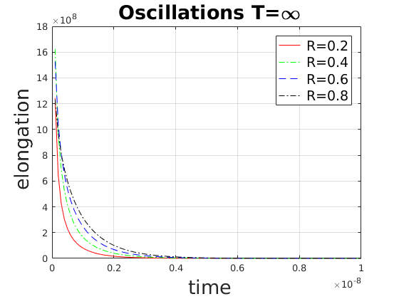 Figure 1
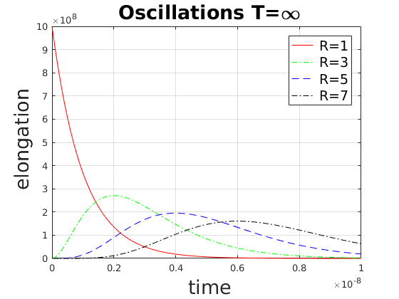 Figure 2
 Figure 3
 Figure 4
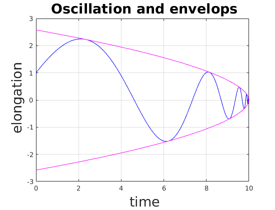 Figure 5
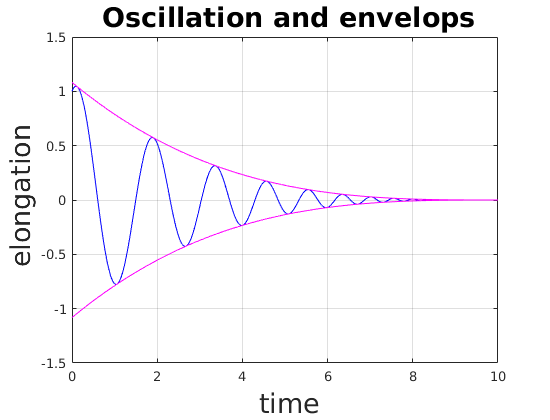 Figure 6
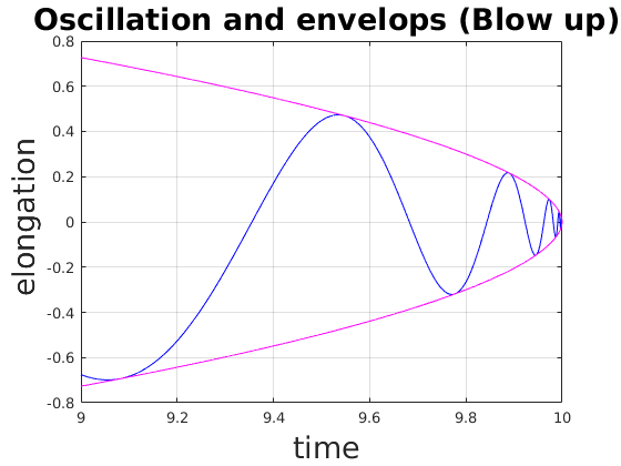 Figure 7
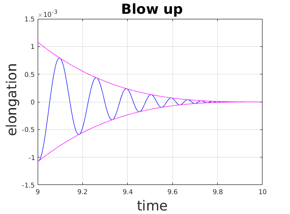 Figure 8
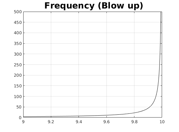 Figure 9
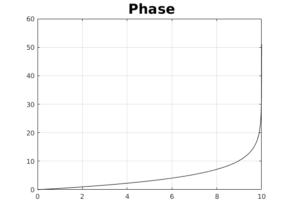 Figure 10
Peer Reviews
No public reviews on file for this paper yet. If you reviewed it on a platform where reviews are public (OpenReview, ICLR, NeurIPS, ICML), you can paste yours below so the community can read it here.
Videos
No videos yet. Explain this paper in a talk, walkthrough, or lecture? Add one.
Taxonomy
TopicsFractional Differential Equations Solutions · Nonlinear Dynamics and Pattern Formation · Differential Equations and Numerical Methods
A representation formula for solutions of second order ode’s with time dependent coefficients
and its application to model dissipative oscillations and waves
Richard Kowar
Department of Mathematics, University of Innsbruck,
Technikerstrasse 21a, A-6020, Innsbruck, Austria
Abstract
In this paper, we model, classify and investigate the solutions of (normalized) second order ode’s with nonconstant continuous coefficients. We introduce a generalized frequency function as the solution of a nonlinear integro-differential equation, show its existence and then derive a representation formula for (all) solutions of (normalized) second order ode’s with nonconstant continuous coefficients. Because this formula specifies the interplay between the coefficients of the ode, the relaxation function (”strongly” decreasing positive function) and the frequency function of the oscillation, it can be applied to design models of dissipative oscillations. As an application, we present and discuss some oscillation models that stop within a finite time period. Moreover, we demonstrate that a large class of oscillations can be used to design and analyze dissipative waves. In particular, it is easy to model dissipative waves that cause in each point of space an oscillation that stops after a finite time period.
1 Introduction
The first main result of this paper is the derivation of a representation formula for solutions of (normalized) second order ode’s with time dependent coefficients and , i.e. solutions of
[TABLE]
where , are continuous functions, is continuous satisfying and . For this purpose, we show that there exists a differentiable frequency function satisfying a nonlinear integro-differential equation such that the solution of (1) (with ) reads as follows
[TABLE]
where
[TABLE]
for and integrable ; and denote time derivative of and the Heaviside function, respectively. We call and the relaxation function and the dissipation function, respectively. It turns out, if and are continuous on , then the existence of this frequency function is always guaranteed. If does not vanish, then the dissipation (of the oscillation) also depends on the frequency and not only on the damping coefficient . We note that there also exists a formula for (cf. Theorem 2 below). This representation formula is a useful tool for designing and analyzing all types of dissipative oscillations. Indeed, from (2), (3) and the equation for (cf. (7) below), we see the interplay between the coefficients and in the ode and the relaxation function and the frequency function of the oscillation. We conclude our analysis of (1) with examples in which we design and discuss oscillations that stop within a finite time period.
In the second part of this paper, we demonstrate that special semigroups of oscillations can be used to design and analyze dissipative waves. For example, a spherical dissipative pressure wave can be modeled by (cf. [15])
[TABLE]
where
[TABLE]
For basic facts about dissipative waves we refer for example to [17, 23, 24, 11, 26, 28, 7, 1, 27, 19, 15]. It seems evident that the elongation, caused by the spherical wave in a space point with , corresponds to an ”oscillation” that starts at time and ends at time for some . Actually, due to , may have a pole at for sufficiently small , i.e. may not be a proper oscillation for small (cf. Example 5).111It seems not reasonable that has a pole for each , but we do not investigate that issue in this paper. At any rate, it stands to reason that there exists a class of oscillations, say , that determines a class of dissipation laws for waves, due to
[TABLE]
Here may be different for different . If or is given, then the associated semigroup of oscillations is defined by
[TABLE]
We investigate the properties that an oscillation must satisfy such that (6) is satisfied for and present some examples.
This paper is organized as follows: In Section 2 we introduce the concept of frequency function related to (1) and show its existence under fairly weak assumptions. Then we tackle the representation formula and the classification of general dissipative oscillations. This section is concluded with some examples. In Section 3, we investigate sufficient conditions for the density and the frequency function such that the respective oscillation determines a dissipation law for dissipative waves. In the appendix, we summarize some notations about the Fourier transform and present a small application of the Paley-Wiener-Schwartz Theorem that is used in our analysis. Finally, the paper is closed with the section Conclusion.
2 Derivation of the representation formular and its application
In this section, we introduce the concept of a frequency function with (and its extension to the real line), which generalizes the frequency and which is a solution of an integro differential equation. Then we show its existence and derive the general representation formula for dissipative oscillations that make use of the frequency function. Moreover, we give a classification of damped oscillations and apply the formula to model dissipative oscillations that stop at a finite time .
According to Chapter VIII in [8], the second order ode with time dependent coefficients (1) has always a twice differentiable solution if and are continuous on . Here denotes the stopping time of the oscillation, which may be finite or infinite.
2.1 The frequency function and the solution formula
Definition 1**.**
Let and be continuous. If there exists a differentiable function satisfying
[TABLE]
*then we call the frequency function of the process modeled by (1). Moreover, we define and .
For applications involving the Fourier transform, it is convenient to extend to the real line by for and for .*
If the coefficient is differentiable, then the condition for the frequency function (7) simplifies to
[TABLE]
and for the special case , we arrive at
[TABLE]
In the following Lemma and Theorem, we show that a frequency function exists if the coefficients and are contiunous and prove the claimed representation formula for the solution of problem (1).
Lemma 1**.**
Let , , be continuous,
- •
* denote the solution of (1) with and ,*
- •
* denote the solution of (1) with and 222Cf. Formula in Theorem 1 below. .*
Then and exist and are twice continuously differentiable on . If , then
[TABLE]
is a real valued frequency function on and satisfies and . If , then
[TABLE]
is an imaginary valued frequency function on and and .
Proof.
Because of the continuity of and , the solutions and exist and are twice continuously differentiable and real valued. In this proof, we denote the distributive derivative of a continuous function by . Then the proof is more instructive.
a) Let . We have to show that
[TABLE]
From (9) together with for , we obtain
[TABLE]
which implies
[TABLE]
and
[TABLE]
Consequently,
[TABLE]
and therefore
[TABLE]
From the definition of and , it follows that , , and and therefore
[TABLE]
This concludes item a).
b) Now let . We note that in (10) can be obtained from (9) if is replaced by . Because satisfies equation , satisfies the same equation and thus identity (11) is also true for this case. Similar as in Item a), the definition of and imply
[TABLE]
which concludes the proof. ∎
Theorem 1**.**
Let , be continuous and be as in Lemma 1 for given and . Then the frequency function is well-defined on with and , and the solution of (1) is given by (2) with and defined by (3).
Proof.
a) Existence. Let , , and be defined as in Lemma 1. The existence of the frequency function on or , respectively, follows from Lemma 1. It is clear that each set and differs from by a countable set of real numbers. In item c) and d) below, we show with the help of the representation formula that or has no zeros on if or holds, respectively.
b) Solution formula. Let with . Because satisfies condition (7), it follows that satisfies the (integrated) characteristic equation of (1), i.e.
[TABLE]
Thus
[TABLE]
are solutions of the equation in (1). Because these solutions are linear independent for non-vanishing , the solution of (1) reads as follows
[TABLE]
From this together with and , we get
[TABLE]
which yields the claimed solution formula.
c) has no zeros on if . From the solution formula and the definition of for , we get
[TABLE]
and thus for all .
d) has no zeros on if . Similarly as before, the solution formula and the definition of and imply
[TABLE]
and hence for all . This concludes the proof. ∎
We now present an example of a purely frequency dependent damped oscillation.
Example 1**.**
Let , , and be a differentiable function that is increasing and that satisfies , and . Moreover, let
[TABLE]
Then , and satisfy condition (7) and for and consequently the solution of (1) is given by
[TABLE]
Because of , it follows that . This example shows that the relaxation function may depend only on the frequency.
Before we consider the second main theorem in this paper, we recall that the function
[TABLE]
for continuous and with is the unique solution of
[TABLE]
due to and . This is a special case of the following result:
Theorem 2**.**
Let , , be as in Lemma 1 and , be as in Theorem 1. Then the solution of (1) with and continuous satisfying is given by
[TABLE]
where , and .
Proof.
It is clear that the solution of
[TABLE]
is equal to for , where solves
[TABLE]
Note that the right hand side corresponds to the ”initial data” and . The claimed formula follows from this and . ∎
2.2 Classification and examples of oscillations
The frequency of a standard oscillation, i.e. the solution of (1) with constant and , is defined by . With this definition the weakly dissipative oscillation the aperiodic limit and creeping can be classified by , and , respectively. This motivates:
Definition 2**.**
Let , , , be as in Definition 1, and be the solution of (1) on .
We call a weakly dissipative oscillation on , if for .
- 2)
We call the solution an aperiodic limit on if for .
- 3)
We call a creeping process on , if for .
- 4)
We call a mixed oscillation, if none of the previous items are true on the whole time interval .
The following example shows that a solution of with need not be damped.
Example 2**.**
*Let , be differentiable with , and be defined by 333If is twice differentiable, then . Then vanishes and the solution of problem (1) reads as follows . Here we assume that and do not both vanish. Although solve the ”damped” oscillation equation with non-vanishing and , it does not describe a damped oscillation. However, its frequency function is not constant.
For example, if for , where and , are positive monotonic increasing functions with , then and . We see that is monotonic increasing with and that is monotonic increasing on for some and . Moreover, the oscillation does not stop at , i.e. not both numbers and vanish.*
In the next two example, we model weakly dissipative oscillations with a finite stopping time . For appropriate initial frequency ( or ), each of these examples reduces to an aperiodic limit or creeping process. But these cases we will not be further investigated.
Example 3**.**
Let , , and be positive, ,
[TABLE]
and
[TABLE]
for . Then , and satisfy identity (7) and the solution of (1) describes an oscillation that is weak dissipative or creeping if or with , respectively. For the special case , we have . Here we focus on the weak dissipative case. According to Theorem 1, the solution of (1) reads as follows
[TABLE]
with
[TABLE]
for . Here we have used that , , , and . We note that
- •
* is strictly increasing if (above we required ) and thus is strictly decreasing,*
- •
* is a linear (and decreasing) if and ;*
- •
if ””, then , and , more precisely, for the limit , we obtain the standard oscillation with constant coefficients.
Two numerical examples are presented in Fig. 1 and Fig. 2 for the setting (i) , , , , and (ii) , , , , , respectively.
The previous example can be generalized as follows.
Example 4**.**
Let , and be positive, and . Then identity (7) is satisfied for , and defined by
[TABLE]
and
[TABLE]
for . Again, the solution of (1) describes an oscillation that is weak dissipative or creeping if or with , respectively. We focus on the weak dissipative case and obtain
[TABLE]
with
[TABLE]
If (as in the above assumption), then is strictly increasing and therefore is strictly decreasing. For a numerical example see Fig. 2.
Remark 1**.**
Apart from the fact that the representation formula enables us to solve any normalized second order ode (with nonconstant coefficients), it is also a very useful tool to model various dissipative oscillations, because it reveals the interplay between the coefficients , , and the damping constant (or equivalently the relaxation function) and the frequency function .
We note that modeling of dissipative oscillations may also involve some requirement about its energy behaviour, but this is beyond the scope of this paper.
3 Modeling dissipative waves with dissipative oscillations
For pure frequency dependent dissipation, the standard dissipative wave equation (cf. [15]) reads as follows
[TABLE]
where is a given dissipation (or complex attenuation) law. Here the operator is defined by , where denotes the Fourier transform of a tempered distribution . We call a function a dissipation law if is nonnegative and even and is odd. We do not assume that the attenuation law is monotonically increasing for positive frequencies and . We also denote the Fourier transform of by . More facts about wave dissipation can be found in [17, 23, 24, 11, 26, 28, 7, 1, 27, 19, 15]. The fundamental solution of the above equation is given by (4) with (5).
We call a semigroup of dissipative oscillations if there exists a dissipation law such that for and for and . Then we have (i) for and (ii) in the distributive sense. As described in the introduction, a dissipative spherical wave is of the form (4) for given .
Moreover, we call a relaxation function if is a positive, monotonic decreasing causal function (, i.e. ) that is an element of .
Proposition 1**.**
Let be a relaxation function satisfying . Then there exists a dissipation law such that .
Proof.
Because , its Fourier transform exists and
[TABLE]
We have to show that there exists a dissipation law satisfying . Such a dissipation law exists, if , is even and is odd. That is even and is odd follows at once from the fact that is real valued. Thus it remains to show that is true.
Visualizing the graph of shows that for , because is positive and decreasing on . As a consequence, does not vanish on . It remains to show that is bounded by . But this property is true, due to
[TABLE]
and the assumption .
Well-definedness of for . Because the complex exponential function satisfies for and , it follows that exists and is well-defined for . ∎
Two of the simplest oscillations are of the form and , where is a relaxation and is a constant frequency. The first one was already considered in the previous proposition, now we consider the second one. For convenience, we define to be if .
Proposition 2**.**
Let be a positive constant, satisfy and for some . Then induces a semigroup of dissipative oscillations by satisfying for .
Proof.
Because , and its Fourier transform exists. According to the proof of Proposition 1, it remains to show that
[TABLE]
From , we infer
[TABLE]
and consequently . Now we show that does not vanish on . From
[TABLE]
and
[TABLE]
we infer
[TABLE]
According to the proof of Proposition 1, is positive and thus does not vanish, too.
The last claim for follows at once from Proposition 3 in the Appendix. Note, is entire, due to . This concludes the proof. ∎
The essential property that we required for the proof of the previous two Propositions was
[TABLE]
Let , , for and for . Then, geometrically, property (15) means that
- (EP)
is not orthogonal to and for all ,
with respect to the scalar product . If is infinite, then we may consider the scalar product on . In summary, we have
Theorem 3**.**
Let be a relaxation function for some satisfying and be a real-valued frequency function. If property (15) or equivalently property (EP) holds, then induces a semigroup of dissipative oscillations by satisfying for .
In the two examples below, we shortly discuss two families of dissipative semigroups.
Example 5**.**
Let with and for , where (cf. Section 3.2 in [9])
[TABLE]
Then for (cf. Exercise 6.3.18 (iii) in [22]) and for . Moreover, let be defined as in (4). In Fig. 3, we have visualized the qualitative behaviour of the ”oscillations” for various values of . We see
- a)
if then has a pole at and is convex444This is not a proper oscillation.,
- b)
if then exists and is positive and convex, and
- c)
if then , is non-negative and has (exactly) one maximum at .
Thus there are three different ”types” of oscillations depending on the distance from the origin of the wave which obey the dissipation law .
Let us now present an example of a relaxation function with support in that can be used to model oscillations with finite stropping time .
Example 6**.**
For example, let be the function from Example 5 and be defined by
[TABLE]
which is -times continuously differentiable on and has support in .
Example 7**.**
Let us shortly consider the semigroup defined by
[TABLE]
where and are positive constants. For the oscillation reduces to the oscillation from the previous example. In contrast to the previous examples, the set of extrem values of is countable. Similarly as in Example 5, has a pole at for and has no pole for .
4 Conclusion
In this paper we performed an analysis of (normalized) second order odes with nonconstant coefficients and derive a solution formular for this type of problem. With this formula we get a much better understanding of dissipative oscillation and their respective models. The essential part of this formular is the existence of a unique (nonnegative) frequency function that satisfies an integro differential equation. If this integro differential equation is fully understood, then dissipative oscillation are also fully understand. Therefore we think that this equation should be analysed in detail by scientists working in the field of integro differential equation or similar fields. Moreover, we demonstrated that the formula is very useful to model or design dissipative oscillations and dissipative waves. As a novelty, we modeled dissipative waves that cause oscillations in each space point that stop after a finite time period.
5 Appendix: Two applications of the Paley-Wiener-Schwartz Theorem
For convenience, we summarize some notation about the Fourier transform and present a small application of the Paley-Wiener-Schwartz Theorem that is used in our analysis of dissipative waves with frequency dependent attenuation laws (cf. [6, 9, 3]).
We use the following form of the Fourier transform of an function
[TABLE]
Then the Convolution Theorem for functions reads as follows
[TABLE]
and, if is differentiable, then
[TABLE]
The inverse Fourier transform is denoted by and . In order to prove that a tempered distribution has support in for some , the following Theorem is essential.
Theorem 4** (Paley-Wiener-Schwartz).**
* has support in if and only if*
- (C1)
* is entire and*
- (C2)
there exist constants and such that
[TABLE]
Let be a dissipation law (of a dissipative wave) and be defined as in (5). If for some finite , then it is clear that holds. Now we show that the structure of the semigroup implies
[TABLE]
Proposition 3**.**
Let and be as in Proposition 1 with the additional assumption for some . Then defined as in (5) satisfies (16).
Proof.
Let and be such that with for each . Then we have with . According to the Paley-Wiener-Schwartz Theorem (Theorem 4 above), we have if and only if (i) is entire and (ii) there exist constants and such that
[TABLE]
Because of property (i) holds. The previous estimation for together with
[TABLE]
for implies
[TABLE]
i.e. , which proves the claim. ∎
The reference list from the paper itself. Each links out to its DOI / PubMed record.
- 1[1] Chen, W and Holm, S.: Fractional Laplacian time-space models for linear and nonlinear lossy media exhibiting arbitrary frequency power-law dependency. J. Acoust. Soc. Am. 115 (4), April 2004.
- 2[2] F. S. Crawford. Berkeley Physik Kurs 3. Schwingungen und Wellen. Vieweg Verlag, Braunschweig, 3. Auflage, 1989.
- 3[3] R. Dautray and J.-L. Lions. Mathematical Analysis and Numerical Methods for Science and Technology. Volume 5. Springer-Verlag , New York, 1992.
- 4[4] W. C. Elmore and M. A. Heald. Physics of Waves. Dover Publications, Inc., New York, 1969.
- 5[5] A. L. Fetter and J.D.Walecka. Theoretical Mechanics of Particles and Continua. Mc Graw-Hill Publishing Company, New York, 1980.
- 6[6] C. Gasquet and P. Witomski. Fourier Analysis and Applications . Springer Verlag, New York, 1999.
- 7[7] Hanyga, A. and Seredynska, M.: Power-law attenuation in acoustic and isotropic anelastic media. Geophys. J. Int , 155:830-838, 2003.
- 8[8] H. Heuser. Gewöhnliche Differentialgleichungen. Teubner, Stuttgart, second edition, 1991.