Convergence issues in derivatives of Monte Carlo null-collision integral formulations: a solution
J-M Tregan (LAPLACE), S. Blanco (LAPLACE), J. Dauchet (IP), M Hafi, (RAPSODEE), R. Fournier (LAPLACE), L Ibarrart (RAPSODEE), P Lapeyre (PROMES),, N Villefranque (CNRM, LAPLACE)

TL;DR
This paper investigates convergence issues in Monte Carlo derivatives of null-collision integral formulations, especially in radiative transfer, and proposes a solution to improve the accuracy of sensitivity evaluations.
Contribution
It identifies convergence problems in Monte Carlo sensitivity analysis for null-collision algorithms and offers a theoretical analysis and an alternative method to address these issues.
Findings
Null-collision algorithms cause convergence difficulties in sensitivity evaluations.
Theoretical analysis reveals why simultaneous Monte Carlo estimators may diverge.
An alternative solution improves the accuracy of derivative estimations.
Abstract
When a Monte Carlo algorithm is used to evaluate a physical observable A, it is possible to slightly modify the algorithm so that it evaluates simultaneously A and the derivatives A of A with respect to each problem-parameter . The principle is the following: Monte Carlo considers A as the expectation of a random variable, this expectation is an integral, this integral can be derivated as function of the problem-parameter to give a new integral, and this new integral can in turn be evaluated using Monte Carlo. The two Monte Carlo computations (of A and A) are simultaneous when they make use of the same random samples, i.e. when the two integrals have the exact same structure. It was proven theoretically that this was always possible, but nothing insures that the two estimators have the same convergence properties: even when a…
Click any figure to enlarge with its caption.
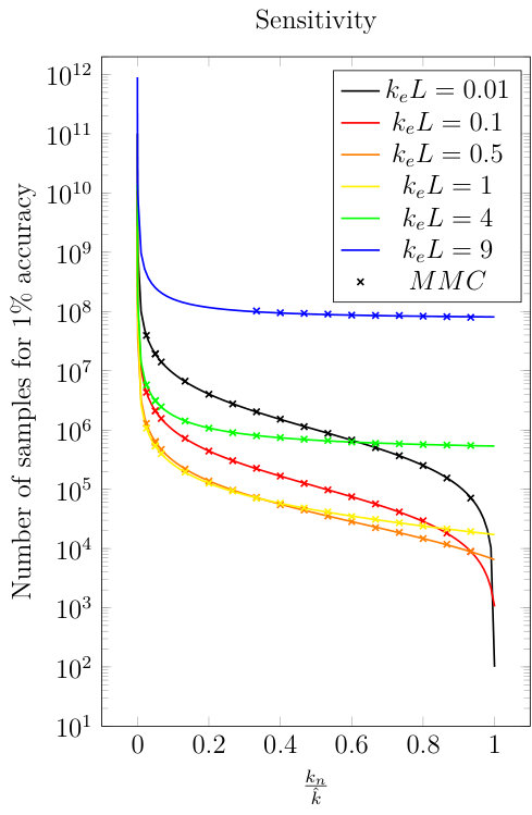 Figure 1
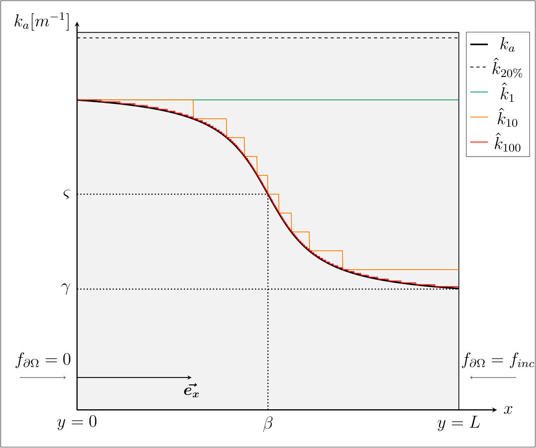 Figure 3
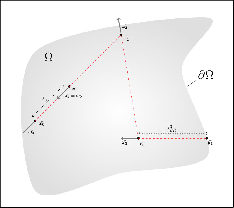 Figure 2
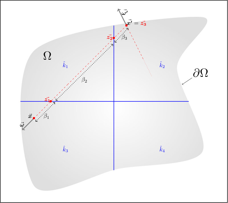 Figure 2
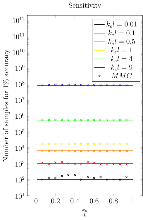 Figure 5
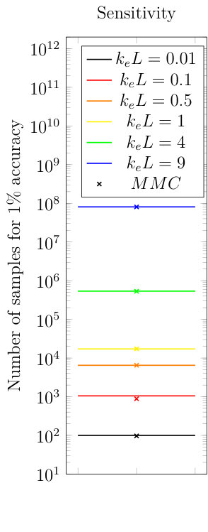 Figure 6
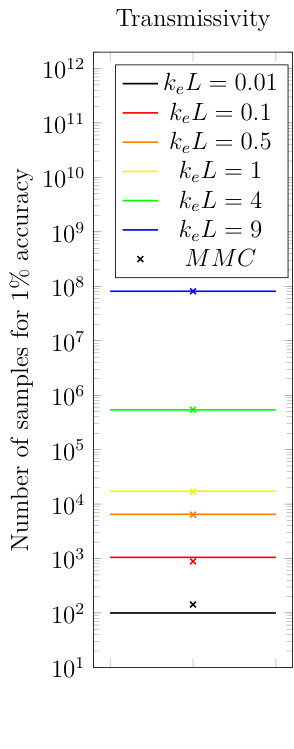 Figure 7
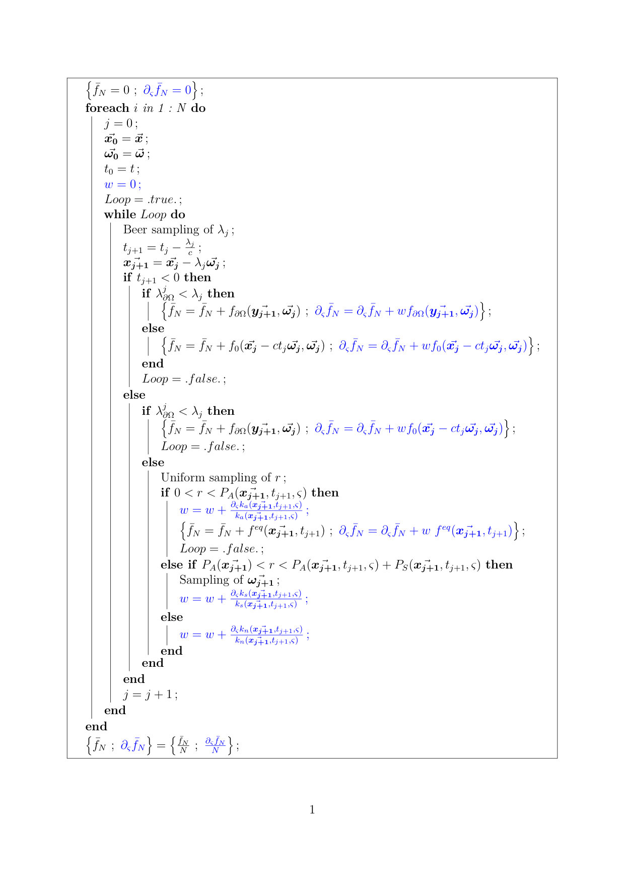 Figure 8
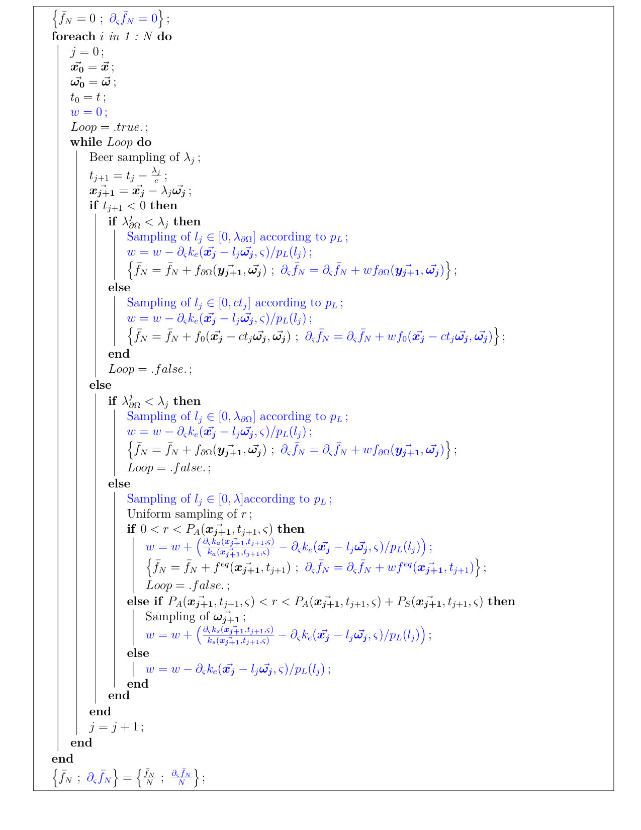 Figure 9
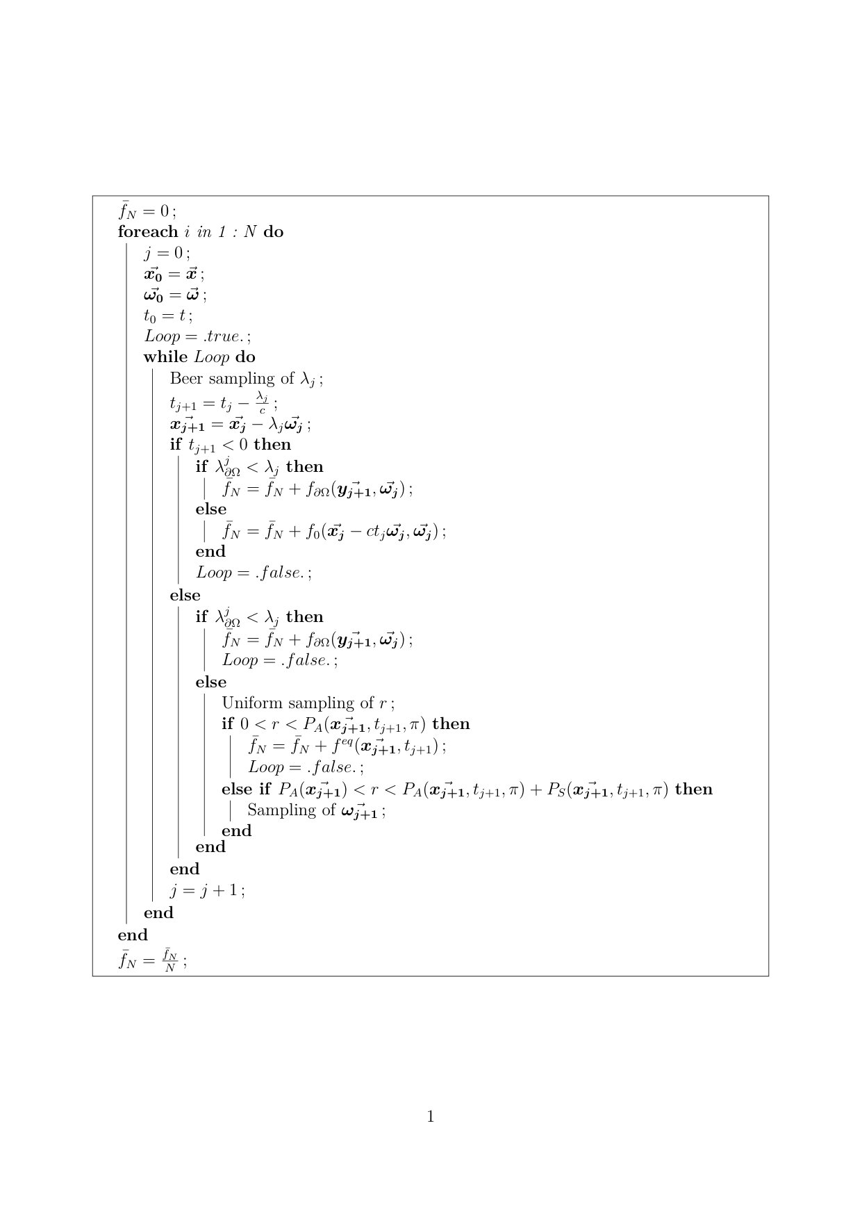 Figure 10
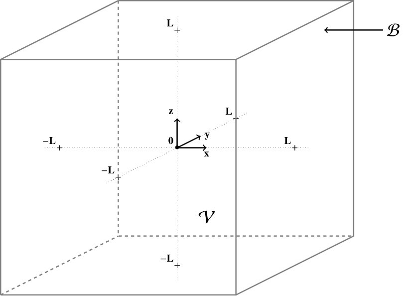 Figure 11
Peer Reviews
No public reviews on file for this paper yet. If you reviewed it on a platform where reviews are public (OpenReview, ICLR, NeurIPS, ICML), you can paste yours below so the community can read it here.
Videos
No videos yet. Explain this paper in a talk, walkthrough, or lecture? Add one.
Taxonomy
TopicsGas Dynamics and Kinetic Theory · Radiation Therapy and Dosimetry · Radiative Heat Transfer Studies
Convergence issues in derivatives of Monte Carlo null-collision integral formulations: a solution
J-M. Tregan
S. Blanco
J. Dauchet
M. El Hafi
R. Fournier
L. Ibarrart
P. Lapeyre
N. Villefranque
LAPLACE, UMR 5213 - Université Paul Sabatier, 118, Route de Narbonne - 31062 Toulouse Cedex, France
Laboratoire RAPSODEE - UMR 5302 - ENSTIMAC - Campus Jarlard - 81013 Albi CT Cedex 09, France
Université Clermont Auvergne, CNRS, SIGMA Clermont, Institut Pascal, F-63000 Clermont-Ferrand, France
PROMES - UPR CNRS 8521 - 7, rue du Four Solaire, 66120 Font Romeu Odeillo, France
Centre National de Recherches Météorologiques (CNRM), UMR 3589 CNRS, Météo France, Toulouse
Laboratoire Plasma et Conversion d’Énergie (LAPLACE), UMR 5213 CNRS, Université Toulouse III
Abstract
When a Monte Carlo algorithm is used to evaluate a physical observable , it is possible to slightly modify the algorithm so that it evaluates simultaneously and the derivatives of with respect to each problem-parameter . The principle is the following: Monte Carlo considers as the expectation of a random variable, this expectation is an integral, this integral can be derivated as function of the problem-parameter to give a new integral, and this new integral can in turn be evaluated using Monte Carlo. The two Monte Carlo computations (of and ) are simultaneous when they make use of the same random samples, i.e. when the two integrals have the exact same structure. It was proven theoretically that this was always possible, but nothing insures that the two estimators have the same convergence properties: even when a large enough sample-size is used so that is evaluated very accurately, the evaluation of using the same sample can remain inaccurate. We discuss here such a pathological example: null-collision algorithms are very successful when dealing with radiative transfer in heterogeneous media, but they are sources of convergence difficulties as soon as sensitivity-evaluations are considered. We analyse theoretically these convergence difficulties and propose an alternative solution.
keywords:
Monte Carlo method , Direct derivatives , Null-collision algorithm , Sensitivity , Integral formulation
MSC:
[2010] 00-01, 99-00
††journal: Journal of LaTeX Templates
1 Introduction
When numerically simulating linear-transport physics using Monte Carlo algorithms, one of the most recurrent difficulties is the handling of highly non-homogenous or fast-variating media. This difficulty was encountered since the beginning of neutron-transport and plasma-physics modelling. But a quite elegant trick was soon identified as a way to bypass this difficulty : virtual collisionners can be added where the true collisionners are scarce so that the total collisionner-density is homogeneous. Of course, in order to ensure that the physical problem is unchanged, when a particle interacts with a virtual collisionner, it simply continues its path as if no collision had occurred [1, 2, 3, 4]. This is the meaning of the denomination null-collision algorithm or fictitious-collision algorithm111Similar keywords are pseudo-collision, null-events, fictitious-events, null-collisions, Woodcock tracking and maximum cross-section. The first practical benefit is that the next collision event can be sampled as if the medium was homogenous. Then the choice is made to select a true-collision or a virtual-collision as function of their local respective-amounts and this is how the spatial information is recovered. But several other benefits were recently foreseen in [1] and practically tested in [5, 6, 7, 8, 9, 10, 11, 12, 13, 14, 15, 16], mainly for radiative-transfer applications. The main idea is that null-collision algorithms transform the non-linearity of Beer-extinction into a linear-recursive problem that Monte Carlo handles without approximation[14]. This was for instance used in [5] to deal with absorption-spectra of molecular gases combining very numerous transitions: the summation over all transitions could be treated by the Monte Carlo algorithm itself, which was previously assumed impossible because this summation was inside the exponential of Beer-extinction. Similarly, the vanishing of the exponential allowed the extension of implicit Monte Carlo algorithms for inversion of absorption and scattering coefficients from intensity measurements [6]. Outside radiative transfer, a very similar idea was used to solve Electromagnetic Maxwell equations for energy propagation in particle-ensembles of statistically-distributed shapes despite of the nonlinearity associated to the square of the electric field[13]. Again similar is the algorithm proposed in [14] solving Boltzmann equation for micro-fluidics applications despite of the nonlinearity of the collision operator.
Back to radiative-transfer applications, the ideas suggested in [1] have motivated significant developments in the computer-graphics community for the cinema industry. Here the benefit of using null-collisions is that it extends to participating media (aerosols or clouds) the orthogonality between data-description and data-treatment that was at the heart of the most recent use of Monte Carlo for rendering complex scenes [7, 9, 8, 10]. The algorithm is indeed processed without any knowledge of the exact spatial-information, and it is only when a collision occurs that access to the field is required: the interaction between the radiative-transfer algorithm and the field-data is strictly restricted to this very moment. This allows the implementation of numerous acceleration techniques with little changes by comparison with those developed for handling complex surfaces. One of these techniques consists in the setting of an acceleration grid, adjusting the amount of virtual collisionners so that the total collisionner-density is both homogeneous in part and close enough to the real density-field. This avoids the sampling of too many useless virtual-collisions. This is one of the starting points of the present paper: null-collision algorithms allow the use of any amount of virtual-collisionners but numerical efficiency justifies that one tries to reduce them to the minimum.
However, we show here that reducing the amount of virtual-collisionners to a minimum leads to convergence difficulties when evaluating sensitivities. Sensitivity evaluation is a very general feature of Monte Carlo techniques: when a Monte Carlo algorithm is used to evaluate a physical observable , it is always possible to modify the algorithm in such a way that it evaluates both and the derivatives of with respect to each problem-parameter , and most commonly the corresponding implementation is quite straightforward [17, 18, 19, 20, 21, 22, 23]222This is not at all straightforward for domain-deformation sensitivities[19, 20], but we here stick to pure parametric sensitivities. But evaluating sensitivities using null-collision algorithms is pathological: the better we adjust the acceleration grid, the worse the statistical convergence rate. In Sec. 2 we will illustrate this pathological behaviour evaluating the transmissivity of a beam through a non-homogeneous column. Then we propose an alternative approach in Sec. 3 where the design of the sensitivity-evaluation algorithm starts from the standard integral solution of the Boltzmann equation, i.e. without virtual-collisionners. The resulting sampling requirements are then addressed with the null-collision approach viewed as a simple rejection-sampling approach. This introduces the cost of sampling an additional random variable, but at this cost the convergence difficulties vanish. We illustrate the numerical behaviour of this modified algorithm is Sec. 4 using a benchmark inspired of [1].
2 Convergence difficulties when evaluating sensitivities
In this section we design a Monte-Carlo algorithm using the standard null-collision approach for the evaluation of the distribution function , i.e. the solution of Boltzmann equation, and apply the technique of [19, 17] for simultaneous evaluation of a sensitivity with respect to , where is a parameter appearing in the absorption and scattering coefficients. The Boltzmann equation that we use is linear with constant speed particles. It matches the monochromatic radiative-transfer equation exactly and all application examples will be restricted to radiative transfer. We choose to make use of the notation instead of the more radiative-transfer oriented notation (the specific intensity) in order to simplify the access for readers of the plasma and neutronics communities. The monochromatic radiative-transfer equation becomes
[TABLE]
where with the location, the propagation direction and the time. For incoming scattering in any direction of the unit sphere , we write and is the single scattering phase function, i.e. is the probability density that the scattering direction is for this incoming direction . The constant particle-speed is and the coefficients , and are the absorption coefficient, the scattering coefficient and the extinction coefficient respectively. is the equilibrium distribution (following the Planck function). is the geometrical domain and its boundary at which the distribution function is known for all locations and all directions of the incoming hemisphere . is the initial condition.
Introducing null-collisions
In order to design a null collision algorithm (NCA)[1] we add a field of virtual collisionners such that the total extinction coefficient is practicable, in the sense that we can sample the corresponding beer extinction:
[TABLE]
where is the null-collision coefficient, is the total extinction-coefficient and is the Dirac distribution. Equation(2) is strictly equivalent to Eq.(1) because of the Dirac distribution that insures .
When numerically adressing the solution of this transport equation at (also solution of Eq.(1)) using the Monte Carlo method, one of the most standard approach consists in a simple statistical reading that allows to view as an average over radiative paths that are tracked backward from the observation location to the sources[1]. In this reading, the pure transport term corresponds to the spatial and temporal propagation of in direction at constant-speed . The collisional term corresponds to either an absorption or a scattering event (including the null-collision events that are forward scattering events). When combining it with the transport term this leads to collision locations that are distributed exponentially along the line of sight (Beer law). Tracking the path backward, this means that the preceeding collision at is at a distance that is a realisation of a random variable of probability density (see Fig. 1). Once is sampled, the collision type is sampled in turn to decide wether an absorption, a true scattering or a null collision occurs. In the backward tracking picture, this corresponds respectively to the three remaining terms
with an absorption event is translated into thermal emission and the algorithm stops with the Monte Carlo weight (the source at ),
- 2.
with a scattering event is translated into the sampling of a “previous” direction and the algorithm continues recursively as if evaluating ,
- 3.
with and its Dirac function, a null collision event is translated into a pure forward scattering event, i.e. the “previous” direction is equal to .
Of course the statistical translation includes the boundary conditions: when backward reaching the boundary at a location and direction , the algorithm stops with the Monte Carlo weight (the incoming source at the boundary). The corresponding Monte Carlo algorithm is detailed in Alg. 1 and illustrated in Fig. 1.
Integral formulation
This null-collision algorithm belongs to the family of analog Monte Carlo algorithms, i.e. algorithms that can be designed without any formal development because they only numerically-implement the well established statistical pictures of radiation physics. However, in the present context it is very much useful to also choose a viewpoint under which the same algorithm appears as a statistical estimate of the integral solution of Eq.(2). For sake of clarity we only write this integral solution at the stationary limit:
[TABLE]
where , , , with the distance to the first boundary-intersection starting at in the direction , i.e. ; where ; . This standard Fredholm equation, typical of the formal solution of linear-transport physics, can be transformed using the following property
[TABLE]
to give
[TABLE]
Then
can be viewed as the probability density function of the free path (the distance until next collision),
- 2.
, and can be viewed as the probabilities that the collision is an absorption, a scattering event or a null-collision respectively,
- 3.
and the two integrals over and can be gathered into a single integral over using the Heaviside function
to give
[TABLE]
with and . This last equation is the integral formulation that we needed in order to construct Alg. 1 at the stationary limit: Alg. 1 is indeed nothing more than the algorithmic-reading of Eq. 5 (and reciprocally Eq. 5 is nothing more than the integral translation of Alg. 1, [18]):
stands for the sampling of the distance of the collision (according to the -field),
- 2.
stands for the case where the sampled collision is outside the boundary, then the algorithm stops at the boundary with the Monte Carlo weight (the value of corresponding to the incoming radiation),
- 3.
stands for the case where the sampled collision is at a location inside the volume, and then three collision types are possible:
- (a)
stands for the case where the collision is an absorption, then the algorithm stops at the boundary with the Monte Carlo weight (the value of at the collision location),
- (b)
stands for the case where the collision is a scattering event, then stands for the sampling of a new direction according to the phase function and the algorithm continues recursively with the estimation of at in direction ,
- (c)
stands for the case where the collision is null, then the algorithm continues recursively with the estimation of at in the unchanged direction
Straightforward application of sensitivity-evaluation techniques
Now that we have constructed the integral formulation of Alg. 1 we can apply the sensitivity-evaluation technique introduced in [17, 19, 20]. It consists in derivating Eq. 5 with respect to and multiplying and dividing by each of the probabilities and probability density functions that depend on . This leads to an integral formulation of the sensitivity that has the very same structure as that of Eq. 5:
[TABLE]
with and . Because of their identical structure, we can gather Eq. 5 and 6 into one using the vectorial notation :
[TABLE]
The algorithmic-reading of 7 leads to Alg. 2 that evaluates simultaneously and . The recursive nature of this algorithm comes from the fact that the final brackets in the scattering and null-collision terms contain and at the same location in the same direction. The fact that their sensitivity part includes a summation is translated into an algorithm incrementing the Monte Carlo weight as explained in Appendix B.
Simulation examples
At this stage, we designed a null-collision algorithm, constructed the corresponding integral formulation and applied the proposition of [17, 19, 20] in a straightforward manner so that the algorithm also evaluates sensitivities. We now test this simulation strategy by evaluating the transmissivity of a non-diffusive heterogeneous column and also evaluating the sensitivity of this transmissivity w.r.t. , a parameter influencing the absorption coefficient. Hereafter this configuration is called heterogeneous-slab (see Fig. 2): is a column of length with the normal incoming at location . The equilibrium distribution is null (cold medium, ). The boundary conditions are and . The absorption and scattering coefficients are and . Alg 2 is used to evaluate both and that correspond to the transmissivity and its derivative respectively: and . We chose this particular profile of , because it is possible to calculate and analytically (see the caption of Fig. 2). Example Monte Carlo results, using samples, are compared to the analytical solution in Tables 5a and 5b. The statistical uncertainty is noted (the standard deviation of the Monte Carlo estimator). In Table 5b we also provide the number of samples required to achieve a accuracy. The simulations were made using five different -profiles (each overestimating at all locations), with acceleration-grids, being uniform within each mesh (see Fig. 2):
for no grid is used: the profile of is uniform, equal to time the maximum -value.
- 2.
for no grid is used: the profile of is again uniform, exactly equal to the maximum -value.
- 3.
for the grid is constructed in such a way that across each mesh the variations of are of the maximum -value, and the profile of is uniform within each mesh, exactly equal to the maximum -value inside the mesh.
- 4.
for and the grid is constructed the same way with and variation respectively.
The transmissivity results of Table 5a confirm that the estimation of is insensitive to the adjustment of the -field (only the computation time is affected). But the sensitivity results of Table 5b clearly indicate the opposite: the statistical convergence is worse when is close to and the number of samples required to reach a given accuracy level can be risen up to infinity when matching to exactly. This is the pathological behavior that we announced in introduction: sensitivities cannot be evaluated accurately when using acceleration grids reducing the number of virtual collisions.
The variance of the sensitivity estimate
For a better understanding of this behavior, we studied a homogeneous-slab for which the variance of the Monte Carlo estimate can be calculated analytically. This case is identical to the previous one (transmissivity of a purely absorbing column) but now is uniform: , and . Of course, there is no need to make use of a null-collision algorithm as soon as is uniform. We only do it for theoretical reasons (with uniform). This allows us to fully identify the reasons why the variance of the sensitivity estimate rises when reducing . This may sound trivial as soon as when encountering a null-collision event, the Monte Carlo weight of the sensitivity algorithm includes a factor (see Eq. 7), but reducing also reduces the number of such null-collision occurrences. This may lead to a compensation, maintaining the variance at a finite value. The developments of appendix A.1 indicate the opposite: the statistical uncertainty is indeed
[TABLE]
Figure 3 illustrates the meaning of this dependance of with the problem parameters. In this idealised case, looking at the behavior of such an algorithm applying sensitivity-evaluation techniques in a straightforward manner, the difficulty is well identified: when approaches zero, the number of samples required for a accurate evaluation of the sensitivity tends to infinity (see Fig. 3c). This figure also displays the behavior of an algorithm implementing the very same sensitivity-evaluation technique, but without the use of null-collisions (which is possible here in this idealised uniform case). Without null-collisions, the relative value of the standard deviation of the sensitivity-estimate (Fig. 3b) is identical to that of the main quantity (the transmissivity-estimate, Fig. 3a). This is an ideal behaviour: the sensitivity is estimated with the same relative accuracy as that of the main quantity. Altogether in this simple example, we see that evaluating sensitivities can be perfectly costless before using null-collisions and may become pathological when null-collisions are introduced.
Note that in the general case, even without null-collisions, evaluating sensitivities can be truely difficult. Understanding the relative variance of sensitivity estimates and comparing them to the relative variance of the algorithm estimating the main quantity was indeed one of the main concerns of the initial work of De Lataillade[17]. Essentially, serious difficulties arise as soon as the scattering optical-thickness is high. The objective of the present paper is not at all to address this specific issue: at the end of the following section, when an alternative solution will be proposed for evaluating sensitivities in null collisions algorithms, the problems associated to highly scattering media will remain unsolved.
3 An alternative approach
The preceding section identifies convergence difficulties when evaluating sensitivities using null-collisions. Theses difficulties are not associated to the standard sensitivity-evaluation algorithm itself: considering slab transmission, we have seen that when we do not make use of null-collisions, the sensitivity-evaluation algorithm converges as well as the algorithm evaluating the main quantity. So the observed difficulties are only the consequences of introducing virtual-collisionners. At this stage, null-collision algorithms appear therefore as perfect tools for handling heterogeneous fields, but are incompatible with the simultaneous evaluation of sensitivities.
We have seen that this problem is related to the term appearing in the Monte Carlo weight of the sensitivity algorithm. At which stage did this term appear and can we bypass this step? Clearly, appeared when derivating with the null-collision probability , with and . A first way to suppress this term consists in making dependent on . This is always possible because is a free parameter and we can therefore adjust it to the variation of so that does not depend on anymore. We first tested this solution and it proved itself already quite practical: the corresponding details are provided in Appendix D. But we finally retained another algorithm, starting from the integral solution of the original Boltzmann Eq. 1, i.e. prior to the introduction of virtual-collisionners. The idea consists in first designing an algorithm evaluating simultaneously and as if the heterogeneity of the field could be handled without difficulty and only introduce null-collisions in a second stage. For this, we can simply rewrite Eq. 5 with (no virtual collisionners):
[TABLE]
The only differences with Eq. 5 are that
,
- 2.
the random variable of probability density (the free path in the -field) is replaced with the random variable of probability density (the free path in the original -field).
This equation can then be derivated with respect to and multiplied/divided by each of the probabilities and probability density functions that depend on (exactly the same way Eq. 7 was constructed from Eq. 5) to give
[TABLE]
A main point of the present paper is that this integral equation, although it was derived the same way as Eq. 7, cannot be interpreted in algorithmic terms: the integral pattern is not yet transformed into a statistical expectation. An additional random generation will be required. At this stage let us introduce an arbitrary random variable of probability density function and write . Reporting this into Eq. 10 and using leads to
[TABLE]
At this stage, null-collisions have not been introduced. Therefore, the algorithmic reading of Eq. 11 would not be practical as soon as the -field is heterogeneous: the difficulty would come from the sampling of . The objective of introducing null collisions will therefore be to replace with another path-length , shorter in average but easy to sample, and compensate the too many collisions by the fact that some of them are null. However, this not as trivial as in the algorithm for the main quantity because of the new random variable that we needed to introduce when transforming Eq. 10 into Eq. 11 (transforming it into an expectation). Indeed needs to be integrated along the whole path, now including null collisions. In statistical terms, this means that the recursivity of the path-sampling algorithm is only insured if the Monte Carlo weight associated to null collisions includes the term , exactly like for true scattering events:
[TABLE]
Equations 5 and 12 have now a similar structure: all the samples used to evaluate can also be used for the evaluation of . But in order to complete the evaluation of sensitivity, we must add one sample (of ) per collision. Thanks to this similar structure, we can gather them into a single vectorial writting (exactly the same way Eq. 7 was constructed from Eq. 5 and 6):
[TABLE]
The algorithmic-reading of 13 leads to Alg. 3 that is an alternative to Alg. 2 for evaluating simultaneously and . As explained in the algorithmic reading of Eq.7, the recursive nature of this algorithm comes from the fact that the final brackets in the scattering and null-collision terms contain and at the same location in the same direction. The fact that their sensitivity part includes a summation is translated into an algorithm incrementing the Monte Carlo weight as explained in B. It is interesting to note that the integral can be more or less difficult to evaluate depending on the profile of . But this can be easily handled using importance sampling based on the -adjustment grid, as explained in C.
4 Simulations using the alternative approach
4.1 Transmissivity of a purely absorbing column
Applying the alternative approach of Sec. 3 to the evaluation of column-transmissivities leads to the content of Fig. 3d and Table 5c. For the homogeneous-slab configuration, Fig. 3 shows that not only the pathological behavior of Sec. 2 is removed, but the sensitivity is estimated with a statistical uncertainty that is perfect for a simultaneous evaluation: its dependence on the parameters of the problem is identical to that of the main quantity. As above, in this very simple case, this uncertainly can be expressed analytically (see A.2) and indeed
[TABLE]
For the heterogeneous-slab configuration, the uncertainty cannot be predicted theoretically, but the conclusions of Fig. 5 are identical to those of Fig. 3: in terms of relative accuracy, the convergence rate is equal to that of the algorithm evaluating the main quantity. It is therefore strictly independent of the adjustment of to . The use of an acceleration grid does only what we expect: it reduces the number of null-collisions but does not impact the variance anymore.
4.2 Full radiative transfer in a 3D configuration
In [1], a cubic benchmark configuration was used to test null-collision algorithms when dealing with three-dimension highly-heterogeneous fields for all ranges of optical thickness and single-scattering albedo. We here make use of the same configuration, named heterogeneous-cube hereafter, in order to test our alternative approach with 3D radiation (see Fig. 4):
radiation is monochromatic;
- 2.
the cube is of side , with black faces;
- 3.
the inside-temperature field is such that varies from (at the center of the face at ) to (at and ) and mimics the shape of flame: (see the profile in Fig. 4);
- 4.
the fields of absorption and scattering coefficients follows the same spatial dependence: and ;
- 5.
The single-scattering phase function is that of Henyey-Greenstein with a uniform value of the asymmetry parameter g;
- 6.
is adjusted to using a regular cubic-grid ( uniform within each mesh): the only parameter for is therefore the number of mesh per direction.
The evaluated quantity is the stationary net-power density and the free physical parameters are , and . In Table 6 we reproduce the computations of Table 1 in [1], i.e. testing wide ranges of optical thicknesses but fixing (isotropic scattering). In the same table we also provide two sensitivities, and , that we evaluated simultaneously with . As in [1], although they are not displayed, we checked that simulation results with non-isotropic scattering lead to the exact same conclusions.
These conclusions are very similar to those reached on the slab-transmissivity example: Table 7 highlights the same features as Fig. 5, the standard deviation of Alg. 3 being independent of , whereas it increases when gets close to for Alg. 2.
5 Conclusion
The simulation examples of the preceding section indicate that the solution proposed in Sec. 3 is practical. Sensitivities can be accurately evaluated even when using null-collision algorithms. We still face convergence difficulties for highly-scattering media, but this is an open question identified in all linear-transport physics, independently of the use of null-collisions.
The way we bypassed the convergence difficulties specific to null-collisions is in rupture with the principle of evaluating sensitivities simultaneously with the main quantity : in all previous works, the two evaluations were truly simultaneous in the sense that the very same samples were used in the and Monte Carlo algorithms. Here, all the samples used to evaluate are also used for the evaluation of , but in order to complete the evaluation of , some additional random variables must be sampled. The sensitivity evaluation has therefore a specific computation-cost. In all our test-cases, this cost was very small compared to the total computation cost, and considering the wide range of tested optical depths we may state that this additional cost has no practical significance for radiative transfer applications. Other linear-transport physicas wold have to be investigated specifically.
In the present text, we only gave very little indications about absolute computer-requirements. We provided some computation-time examples in Fig. 6, without the use of any acceleration grid. Most of our analysis was made with another measure: the average number of random generation per path, which should be proportional to the computation time, but only once all optimisations will be implemented. As illustrated in [7, 9, 8, 10], such data-access considerations in relation with null-collision algorithms (i.e the time associated to a close adjustment of to ) is an ongoing computer-science research. The question of implementing the corresponding tools (developped by the computer-graphics community) together with the present sensitivity evaluation algorithm will be discussed in a separate paper.
Appendix A Analytical variances for homogeneous-slab
is a slab of length with the incoming normal at location and as boundary condition (see figure 2). The equilibrium distribution is null (no emssion) and the absorption and scattering coefficients are and . The transmissivity is .
A.1 For the standard approachs
Using Eq.(7),
[TABLE]
To get the analytical variance for the standard approach (Alg. 2) in homogeneous-slab, we started by designing a countable categorisation of paths: () is the set of paths that crossed the column and met null-collisions and all other paths (path without null-collisions). The probability that a path belongs to the category is
p_{n}=\frac{\hat{k}^{n}}{n!}L^{n}\mathrm{e}^{-\hat{k}L}\Big{(}1-\frac{k_{a}(\varsigma)}{\hat{k}}\Big{)}
The Monte Carlo weight obtained at the end of a path belonging to the is
The weight of a path belonging to is zero. Therefore, the variance of the Alg. 2 is
[TABLE]
A.2 For the alternative approach
Using Eq.(13),
[TABLE]
The variance of a Bernoulli law of parameter is , and therefore the variance of Alg. 3 is
[TABLE]
Similarly for Alg. 1,
[TABLE]
Appendix B Incrementation of the Monte Carlo weights
The standard approach of Alg. 2 is designed from the algorithmic-reading of Eq. 7 and the recursive nature of this algorithm comes from the fact that the final brackets in the scattering and null-collision terms contain and at the same location in the same direction. As the integral formulation of and have identical structures, we can just use one unique sampled-path to evaluate simultaneously and . For a better understanding of the meaning of this unique sampled-path, we express here the Monte Carlo weight for one path example: the path displayed in Fig. 1, i .e. one null-collision at location , two scatterings at location and , and one boundary-collision at location . Thanks to the algorithmic-reading of Eq. 7, after one null-collision at location . The notations are simplified by writing instead of . We have
[TABLE]
At this stage, and need to be evaluated at the same location () in the same direction (). According to Eq. 7, it’s possible to use the same path to evaluate and . Therefore, after one scattering-collision at location in direction , we have and ,
[TABLE]
Similarly, after one scattering at location in direction ,
[TABLE]
and after the boundary-collision at location in direction ,
[TABLE]
where and . The summation of and is therefore translated into an algorithm incrementing the Monte Carlo weight. This is how the Monte Carlo weight is incremented in the fully recursive algorithm of Alg. 3.
Appendix C The additional sampling
To evaluate with the alternative approach of Alg. 3, we must evaluate . We make use of one additional sampling:
[TABLE]
However, depending on the the profile of , this integral can be source of variance if the spatial variations of do not sufficiently match those . We did not yet adress this importance-sampling issue and bypassed it using stratified sampling: we increased the number of ”collisions” by including the grid-intersections to write
[TABLE]
where is the number of grid-intersections along the path . For all , is the location of the ”collision”, is the length between two successive ”collisions” and (see Fig. 8).
This stratified sampling is only meaningful if we assume that the grid is sufficiently refined to capture the spatial variation of . But initially, the grid was only designed to reduce the amount of null-collisions. Therefore, another grid-refinement criterium should be introduced if this strategy is retained. But again, stratified sampling is not the only possible solution and the grid may be used differently: make pre-computations in each mesh and sample only once along the whole path using importance sampling, which would suppress the increase of computation costs when refining the grid in Fig. 5 ( increasing in Fig. 5c).
Appendix D Another possible approach: varying with
In Eq. (5), we chose to use a constant upper bound of noted . Nevertheless, nothing prevents us from varying according to the parameter , while preserving the fact that is independent of space in order to still enable an easy sampling of . Thus, we have complete freedom in the choice of these variations, and we will choose them to reduce the variance as much as possible.
In addition, we have shown that the explosion is due to the fact that Monte Carlo’s weight includes a factor . This factor appeared when applying the sensitivity evaluation technique to Eq. (5), especially because of the term \partial_{\varsigma}\Big{(}\frac{k_{n}}{\hat{k}}\Big{)}.
Therefore, and now that depends on , we may impose \partial_{\varsigma}\Big{(}\frac{k_{n}}{\hat{k}}\Big{)}=0, which implies the following relation:
[TABLE]
Thus, by derivating Eq. (5), we obtain:
[TABLE]
with
We have implemented the algorithm resulting from this integral formulation and compared it with the approach proposed in the core of the present paper. Whatever the case, it was always less efficient.
Acknowledgments
We acknowledge support from the Agence Nationale de la Recherche (ANR, grant HIGH-TUNE ANR-16-CE01-0010, http://www.umr-cnrm.fr/high-tune), from the french Programme National de Teledetection Spatiale (PNTS-2016-05), from Region Occitanie (Projet CLE-2016 EDStar) and from the French Minister of Higher Education, Research and Innovation for the PhD scholarship of the first author.
References
- [1]
M. Galtier, S. Blanco, C. Caliot, C. Coustet, J. Dauchet, M. El Hafi, V. Eymet, R. Fournier, J. Gautrais, A. Khuong, et al., Integral formulation of null-collision monte carlo algorithms, Journal of Quantitative Spectroscopy and Radiative Transfer 125 (2013) 57–68.
- [2]
H. Skullerud, The stochastic computer simulation of ion motion in a gas subjected to a constant electric field, Journal of Physics D: Applied Physics 1 (11) (1968) 1567.
- [3]
E. Woodcock, T. Murphy, P. Hemmings, S. Longworth, Techniques used in the gem code for monte carlo neutronics calculations in reactors and other systems of complex geometry, in: Proc. Conf. Applications of Computing Methods to Reactor Problems, Vol. 557, 1965.
- [4]
S. Lin, J. Bardsley, The null-event method in computer simulation, Computer Physics Communications 15 (3-4) (1978) 161–163.
- [5]
M. Galtier, S. Blanco, J. Dauchet, M. El Hafi, V. Eymet, R. Fournier, M. Roger, C. Spiesser, G. Terrée, Radiative transfer and spectroscopic databases: A line-sampling monte carlo approach, Journal of Quantitative Spectroscopy and Radiative Transfer 172 (2016) 83–97.
- [6]
M. Galtier, M. Roger, F. André, A. Delmas, A symbolic approach for the identification of radiative properties, Journal of Quantitative Spectroscopy and Radiative Transfer 196 (2017) 130–141.
- [7]
P. Kutz, R. Habel, Y. K. Li, J. Novák, Spectral and decomposition tracking for rendering heterogeneous volumes, ACM Transactions on Graphics (TOG) 36 (4) (2017) 111.
- [8]
J. Novák, I. Georgiev, J. Hanika, W. Jarosz, Monte carlo methods for volumetric light transport simulation, in: Computer Graphics Forum, Vol. 37, Wiley Online Library, 2018, pp. 551–576.
- [9]
J. Novák, A. Selle, W. Jarosz, Residual ratio tracking for estimating attenuation in participating media., ACM Trans. Graph. 33 (6) (2014) 179–1.
- [10]
M. Raab, D. Seibert, A. Keller, Unbiased global illumination with participating media, in: Monte Carlo and Quasi-Monte Carlo Methods 2006, Springer, 2008, pp. 591–605.
- [11]
J. Dauchet, J.-J. Bézian, S. Blanco, C. Caliot, J. Charon, C. Coustet, M. El Hafi, V. Eymet, O. Farges, V. Forest, et al., Addressing nonlinearities in monte carlo, Scientific reports 8 (1) (2018) 13302.
- [12]
J. Dauchet, S. Blanco, J.-F. Cornet, M. El Hafi, V. Eymet, R. Fournier, The practice of recent radiative transfer monte carlo advances and its contribution to the field of microorganisms cultivation in photobioreactors, Journal of Quantitative Spectroscopy and Radiative Transfer 128 (2013) 52–59.
- [13]
J. Charon, S. Blanco, J.-F. Cornet, J. Dauchet, M. El Hafi, R. Fournier, M. K. Abboud, S. Weitz, Monte carlo implementation of schiff׳ s approximation for estimating radiative properties of homogeneous, simple-shaped and optically soft particles: Application to photosynthetic micro-organisms, Journal of Quantitative Spectroscopy and Radiative Transfer 172 (2016) 3–23.
- [14]
G. Terrée, M. E. Hafi, S. Blanco, R. Fournier, J. Dauchet, J. Gautrais, Addressing the gas kinetics boltzmann equation with branching paths statistics, arXiv preprint arXiv:1712.02900.
- [15]
N. Villefranque, F. Couvreux, R. Fournier, S. Blanco, C. Cornet, V. Eymet, V. Forest, J.-M. Tregan, Path-tracing Monte Carlo Libraries for 3D Radiative Transfer in Cloudy Atmospheres, arXiv e-prints (2019) arXiv:1902.01137arXiv:1902.01137.
- [16]
J. Dauchet, S. Blanco, J.-F. Cornet, R. Fournier, Calculation of the radiative properties of photosynthetic microorganisms, Journal of Quantitative Spectroscopy and Radiative Transfer 161 (2015) 60–84.
- [17]
A. De Lataillade, S. Blanco, Y. Clergent, J.-L. Dufresne, M. El Hafi, R. Fournier, Monte carlo method and sensitivity estimations, Journal of Quantitative Spectroscopy and Radiative Transfer 75 (5) (2002) 529–538.
- [18]
J. Delatorre, G. Baud, J.-J. Bézian, S. Blanco, C. Caliot, J.-F. Cornet, C. Coustet, J. Dauchet, M. El Hafi, V. Eymet, et al., Monte carlo advances and concentrated solar applications, Solar Energy 103 (2014) 653–681.
- [19]
M. Roger, S. Blanco, M. El Hafi, R. Fournier, Monte carlo estimates of domain-deformation sensitivities, Physical review letters 95 (18) (2005) 180601.
- [20]
M. Roger, M. El Hafi, R. Fournier, S. Blanco, A. De Lataillade, V. Eymet, P. Perez, Applications of sensitivity estimations by monte carlo methods, in: ICHMT DIGITAL LIBRARY ONLINE, Begel House Inc., 2004.
- [21]
S. Blanco, R. Fournier, Short-path statistics and the diffusion approximation, Physical review letters 97 (23) (2006) 230604.
- [22]
G. Terrée, S. Blanco, M. El Hafi, R. Fournier, J. Y. Rolland, Diffusion approximation and short-path statistics at low to intermediate knudsen numbers, EPL (Europhysics Letters) 110 (2) (2015) 20007.
- [23]
G. Mikhailov, Optimization of Weighted Monte Carlo Methods, Springer-Verlag, 1995.
The reference list from the paper itself. Each links out to its DOI / PubMed record.
- 1[1] M. Galtier, S. Blanco, C. Caliot, C. Coustet, J. Dauchet, M. El Hafi, V. Eymet, R. Fournier, J. Gautrais, A. Khuong, et al., Integral formulation of null-collision monte carlo algorithms, Journal of Quantitative Spectroscopy and Radiative Transfer 125 (2013) 57–68.
- 2[2] H. Skullerud, The stochastic computer simulation of ion motion in a gas subjected to a constant electric field, Journal of Physics D: Applied Physics 1 (11) (1968) 1567.
- 3[3] E. Woodcock, T. Murphy, P. Hemmings, S. Longworth, Techniques used in the gem code for monte carlo neutronics calculations in reactors and other systems of complex geometry, in: Proc. Conf. Applications of Computing Methods to Reactor Problems, Vol. 557, 1965.
- 4[4] S. Lin, J. Bardsley, The null-event method in computer simulation, Computer Physics Communications 15 (3-4) (1978) 161–163.
- 5[5] M. Galtier, S. Blanco, J. Dauchet, M. El Hafi, V. Eymet, R. Fournier, M. Roger, C. Spiesser, G. Terrée, Radiative transfer and spectroscopic databases: A line-sampling monte carlo approach, Journal of Quantitative Spectroscopy and Radiative Transfer 172 (2016) 83–97.
- 6[6] M. Galtier, M. Roger, F. André, A. Delmas, A symbolic approach for the identification of radiative properties, Journal of Quantitative Spectroscopy and Radiative Transfer 196 (2017) 130–141.
- 7[7] P. Kutz, R. Habel, Y. K. Li, J. Novák, Spectral and decomposition tracking for rendering heterogeneous volumes, ACM Transactions on Graphics (TOG) 36 (4) (2017) 111.
- 8[8] J. Novák, I. Georgiev, J. Hanika, W. Jarosz, Monte carlo methods for volumetric light transport simulation, in: Computer Graphics Forum, Vol. 37, Wiley Online Library, 2018, pp. 551–576.