Gravitationally Lensed Quasar SDSS J1442+4055: Redshifts of Lensing Galaxies, Time Delay, Microlensing Variability, and Intervening Metal System at z ~ 2
Vyacheslav N. Shalyapin, Luis J. Goicoechea

TL;DR
This study measures the time delay, microlensing effects, and intervening metal absorption in the gravitationally lensed quasar SDSS J1442+4055, providing data useful for cosmology and galaxy evolution studies.
Contribution
It presents new spectroscopic and photometric measurements of the lens system, including a precise time delay and characterization of the intervening metal-rich absorber.
Findings
Time delay of 25.0 ± 1.5 days between images A and B.
Detection of a dust extinction bump at 2209 Å in the intervening system.
Spectroscopic confirmation of the lensing galaxy at z = 0.284.
Abstract
We present an --band photometric monitoring of the two images A and B of the gravitationally lensed quasar SDSS J1442+4055 using the Liverpool Telescope (LT). From the LT light curves between 2015 December and 2018 August, we derive at once a time delay of 25.0 1.5 days (1 confidence interval; A is leading) and microlensing magnification gradients below 10 mag day. The delay interval is not expected to be affected by an appreciable microlensing--induced bias, so it can be used to estimate cosmological parameters. This paper also focuses on new Gran Telescopio Canarias (GTC) and LT spectroscopic observations of the lens system. We determine the redshift of two bright galaxies around the doubly imaged quasar using LT spectroscopy, while GTC data lead to low--noise individual spectra of A, B, and the main lensing galaxy G1. The G1 spectral shape is accurately…
Click any figure to enlarge with its caption.
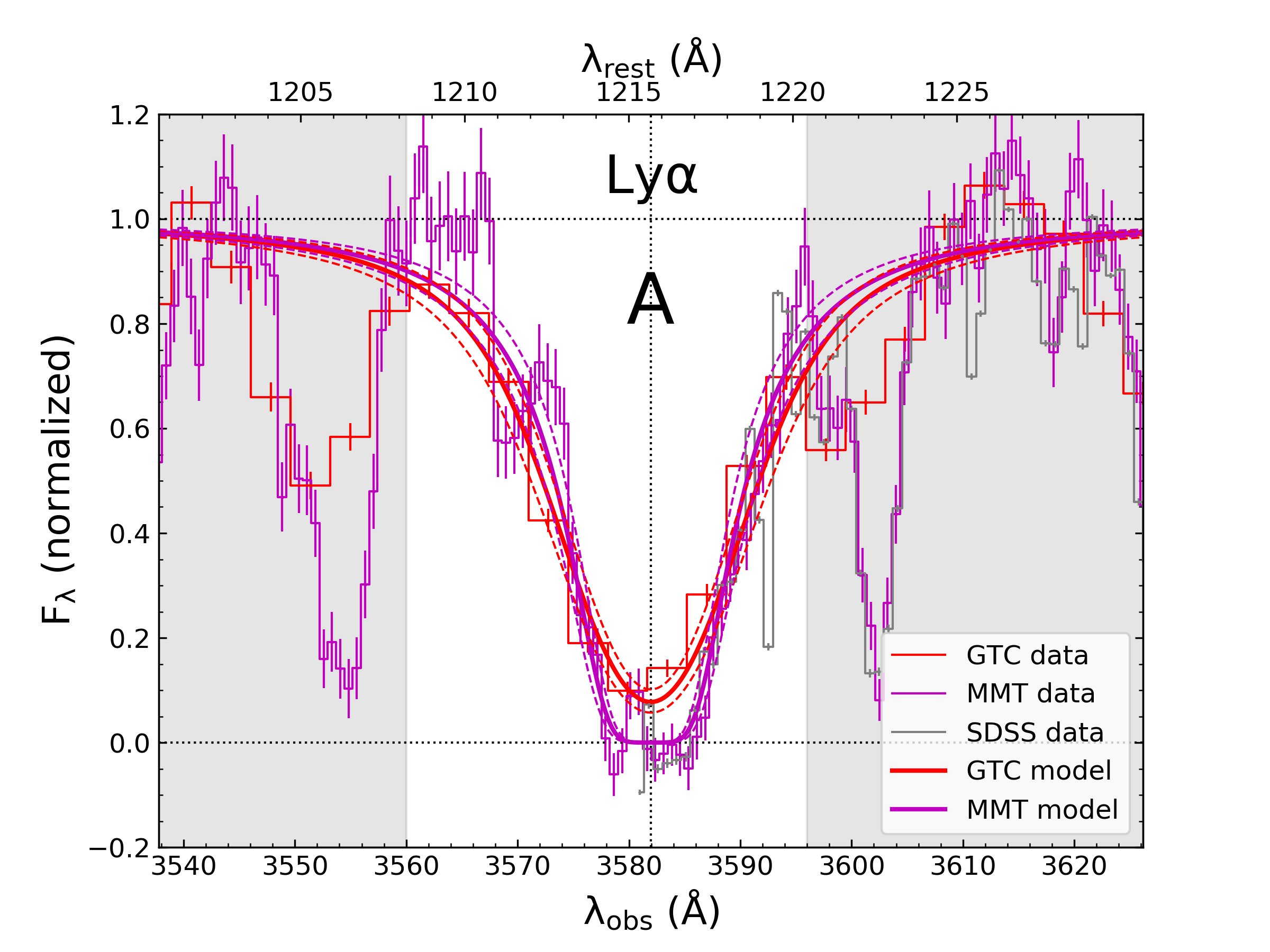 Figure 1
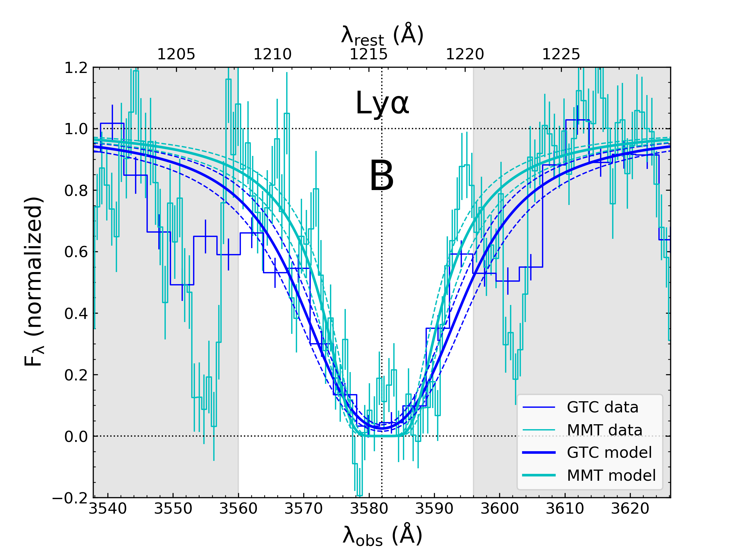 Figure 2
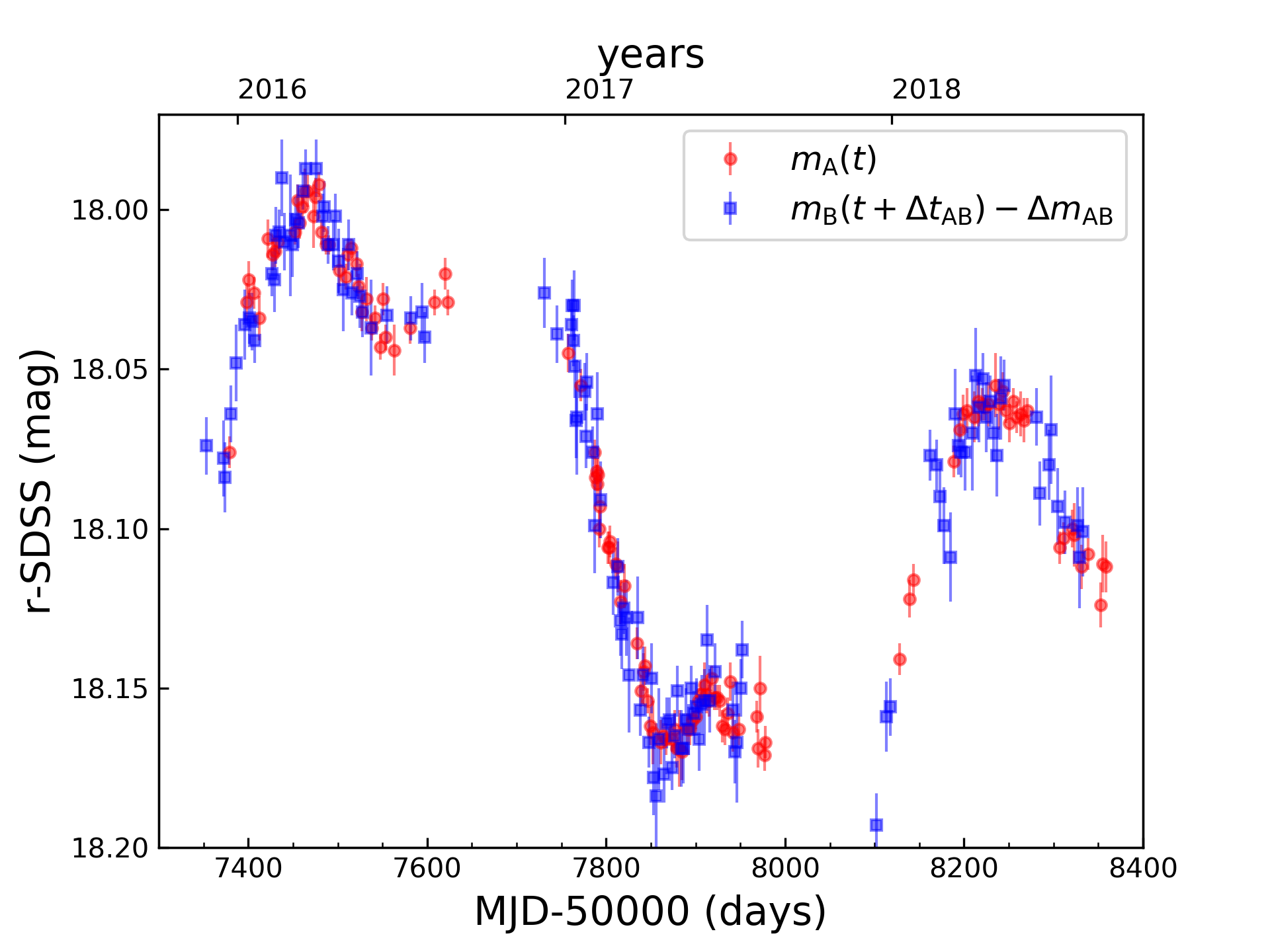 Figure 3
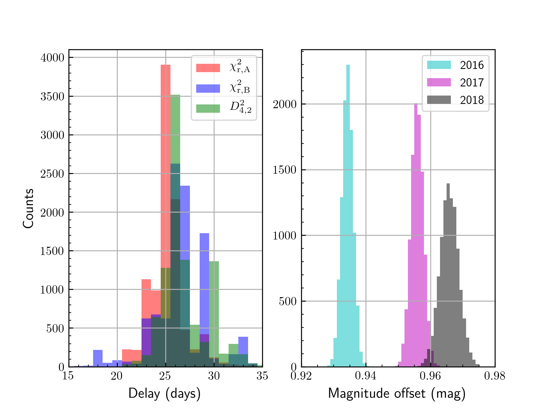 Figure 4
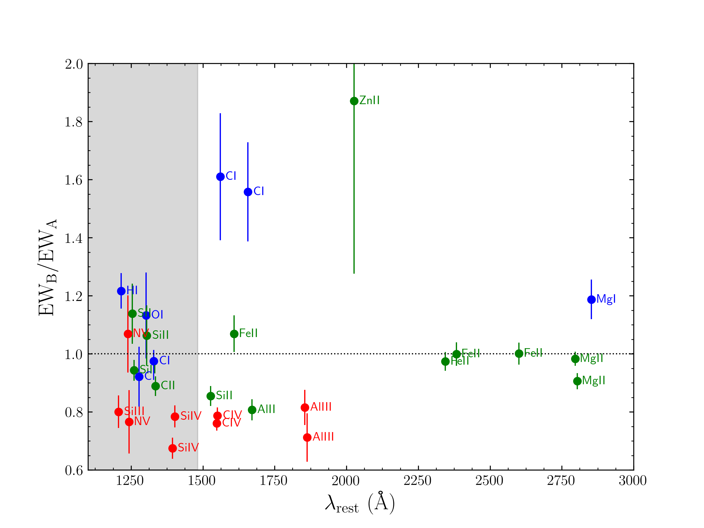 Figure 5
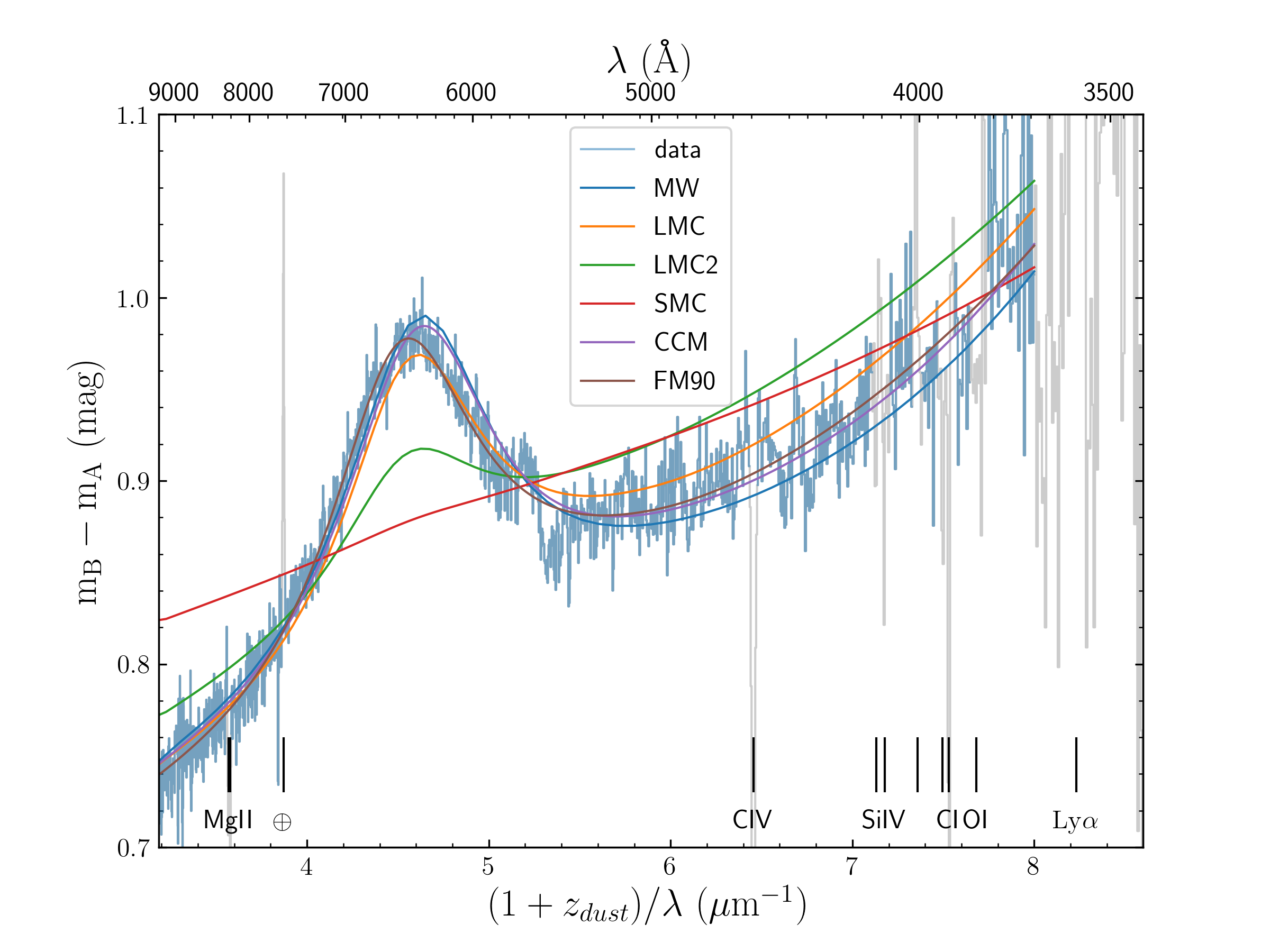 Figure 6
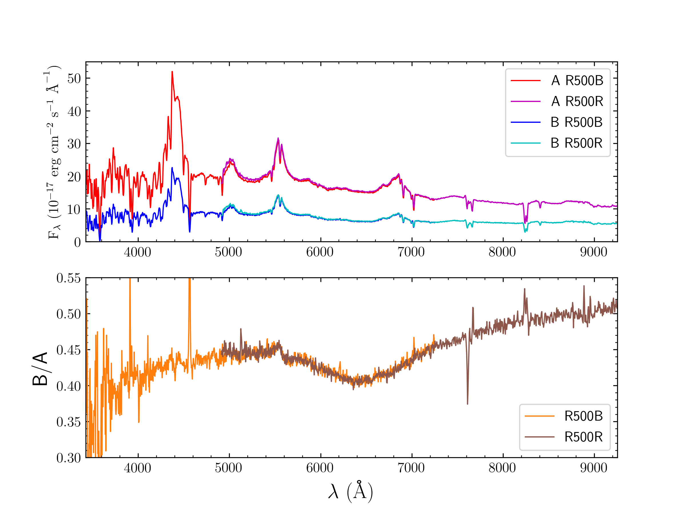 Figure 7
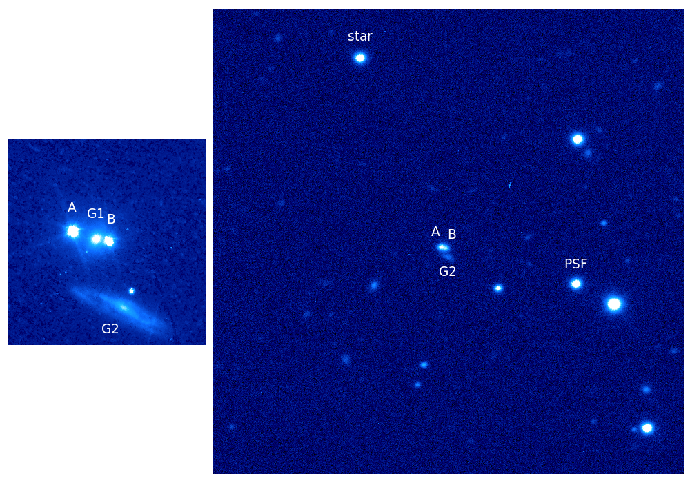 Figure 8
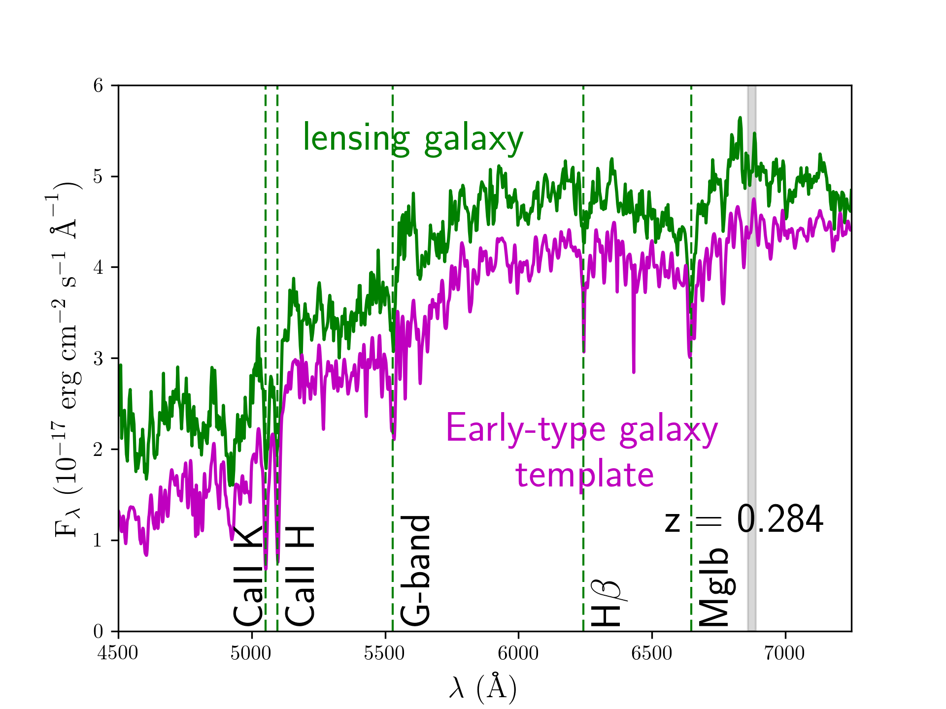 Figure 9
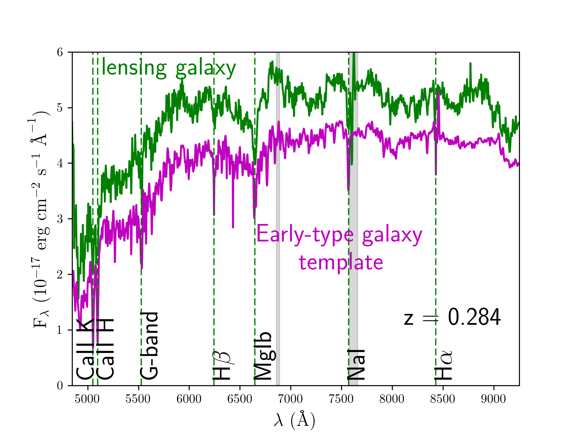 Figure 10
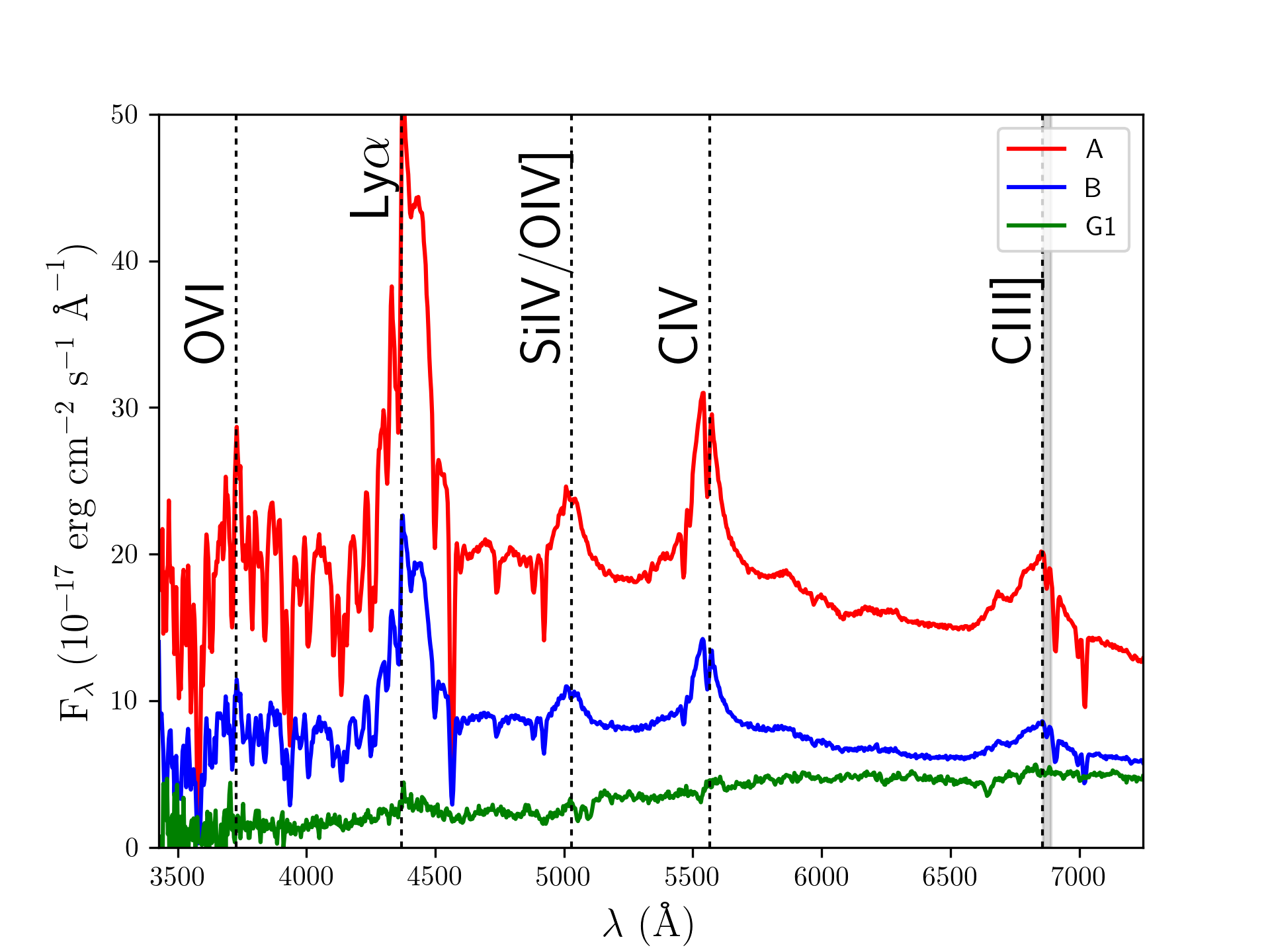 Figure 11
 Figure 12
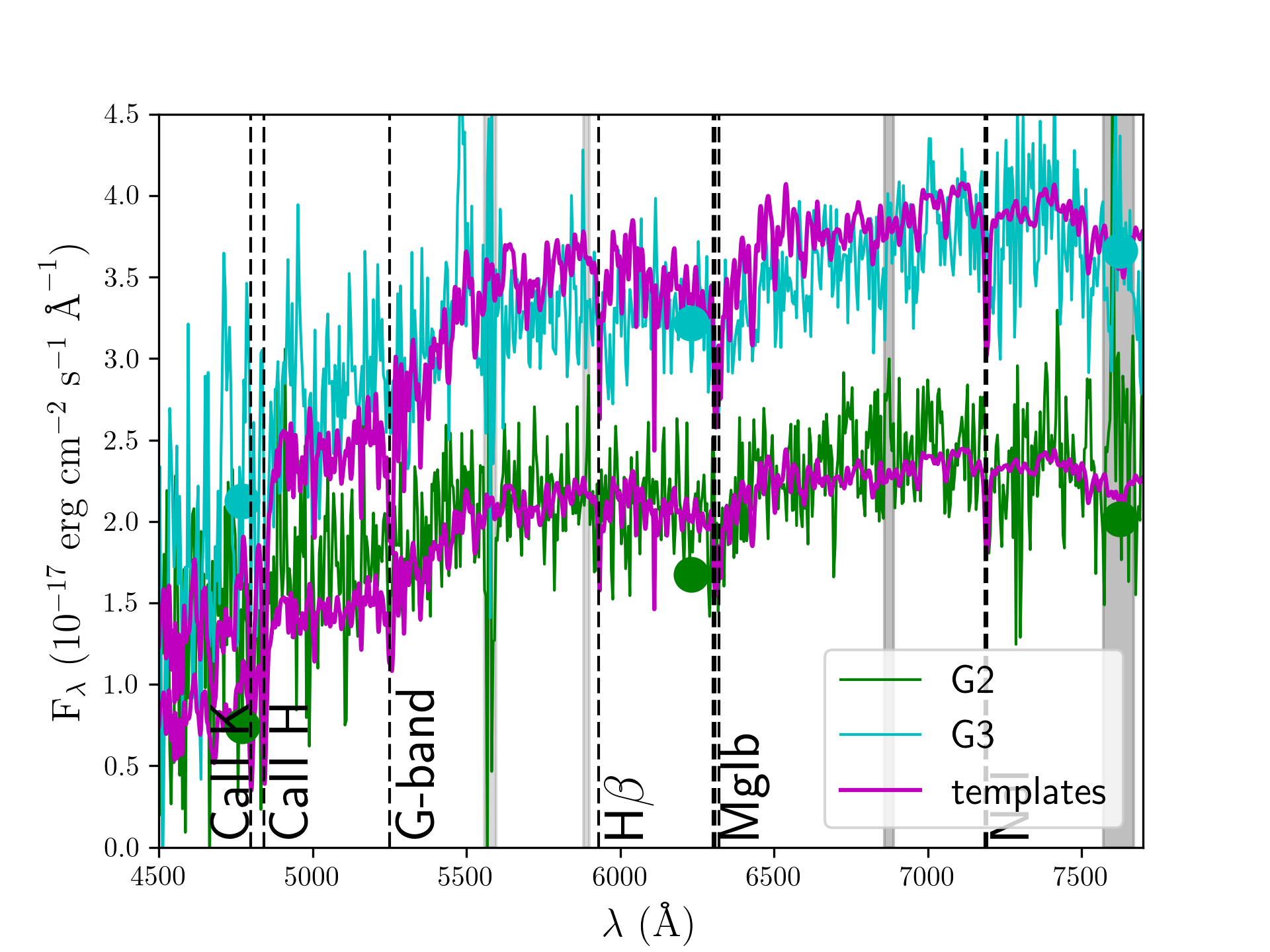 Figure 13
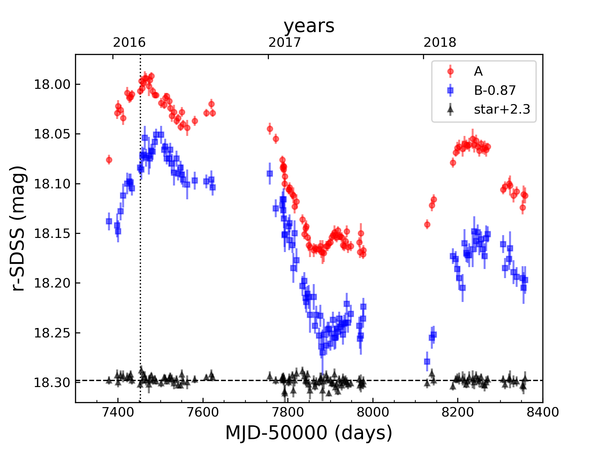 Figure 14
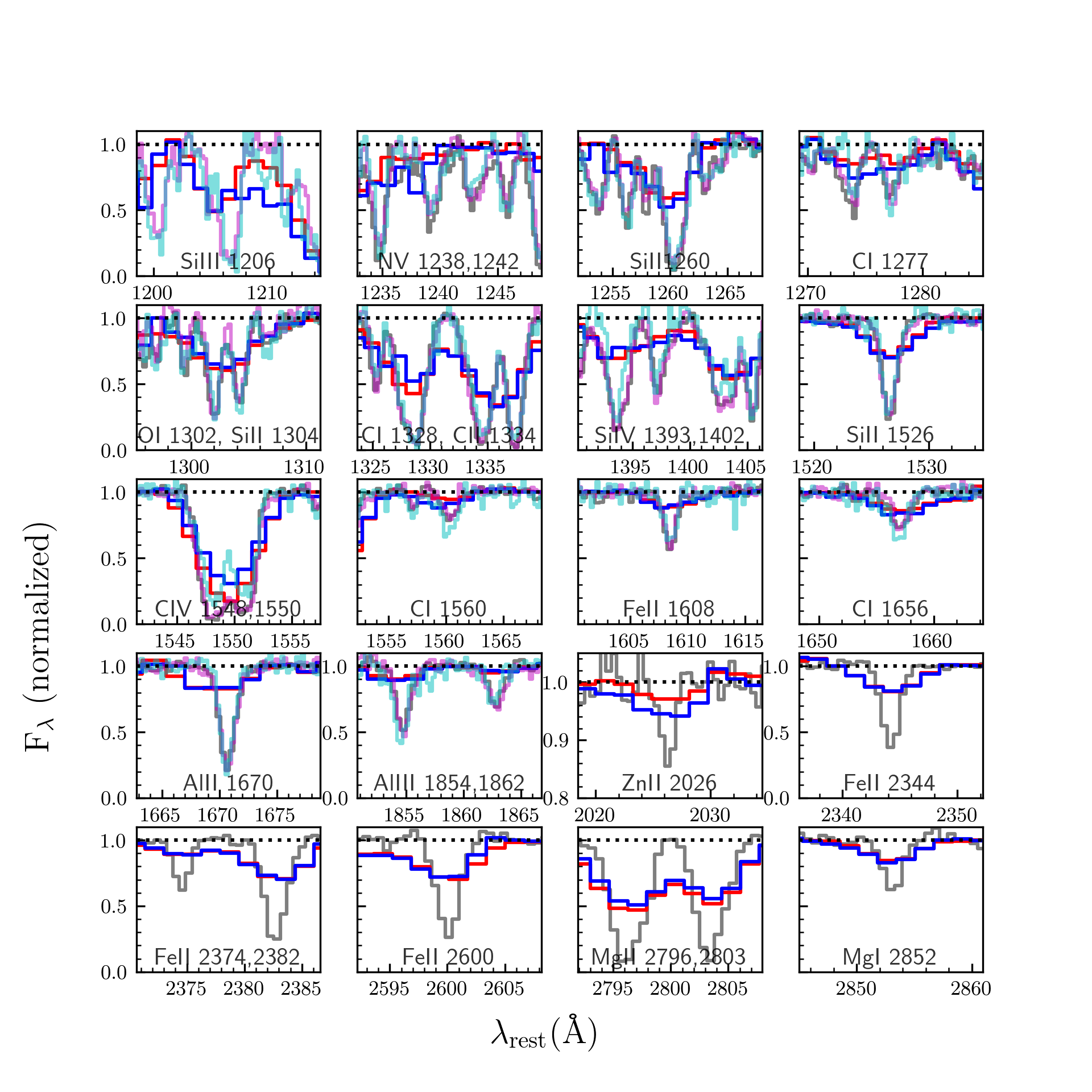 Figure 15
| MJD–50000 | aa–SDSS magnitude. | aa–SDSS magnitude. | aa–SDSS magnitude. | aa–SDSS magnitude. | ababfootnotemark: | ababfootnotemark: |
|---|---|---|---|---|---|---|
| 7379.288 | 18.076 | 0.005 | 19.008 | 0.009 | 15.998 | 0.004 |
| 7398.293 | 18.029 | 0.006 | 19.012 | 0.012 | 15.993 | 0.006 |
| 7400.289 | 18.022 | 0.006 | 19.018 | 0.011 | 16.000 | 0.005 |
| 7406.279 | 18.026 | 0.005 | 18.998 | 0.009 | 15.993 | 0.005 |
| 7412.267 | 18.034 | 0.007 | 18.982 | 0.012 | 15.994 | 0.006 |
| aaObserved wavelength in Å. | (A)bbWe use S to denote the field (control) star. | (A)ccFlux error in 10-17 erg cm-2 s-1 Å-1. | (B)bbFlux in 10-17 erg cm-2 s-1 Å-1. | (B)ccFlux error in 10-17 erg cm-2 s-1 Å-1. | (G1)bbFlux in 10-17 erg cm-2 s-1 Å-1. | (G1)ccFlux error in 10-17 erg cm-2 s-1 Å-1. |
|---|---|---|---|---|---|---|
| 3426.770 | 17.928 | 1.660 | 14.001 | 1.520 | -10.045 | 1.694 |
| 3430.330 | 19.053 | 1.569 | 9.429 | 1.446 | -3.607 | 1.645 |
| 3433.891 | 19.969 | 1.490 | 8.143 | 1.324 | 0.734 | 1.571 |
| 3437.452 | 17.532 | 1.420 | 9.126 | 1.259 | -3.928 | 1.449 |
| 3441.013 | 21.708 | 1.435 | 7.852 | 1.201 | -2.417 | 1.424 |
| aaObserved wavelength in Å. | (A)bbFlux in 10-17 erg cm-2 s-1 Å-1. | (A)ccFlux error in 10-17 erg cm-2 s-1 Å-1. | (B)bbFlux in 10-17 erg cm-2 s-1 Å-1. | (B)ccFlux error in 10-17 erg cm-2 s-1 Å-1. | (G1)bbFlux in 10-17 erg cm-2 s-1 Å-1. | (G1)ccFlux error in 10-17 erg cm-2 s-1 Å-1. |
|---|---|---|---|---|---|---|
| 4846.734 | 22.387 | 0.362 | 9.399 | 0.274 | 4.743 | 0.305 |
| 4851.550 | 22.515 | 0.358 | 9.669 | 0.271 | 4.009 | 0.300 |
| 4856.365 | 23.775 | 0.353 | 9.587 | 0.265 | 4.339 | 0.293 |
| 4861.180 | 24.849 | 0.346 | 10.300 | 0.261 | 4.242 | 0.287 |
| 4865.995 | 23.896 | 0.322 | 10.484 | 0.243 | 2.466 | 0.260 |
| aaObserved wavelength in Å. | (G2)bbFlux in 10-17 erg cm-2 s-1 Å-1. | (G3)bbFlux in 10-17 erg cm-2 s-1 Å-1. |
|---|---|---|
| 3984.359 | 6.368 | -5.175 |
| 3988.991 | 12.435 | 4.964 |
| 3993.623 | 3.922 | 3.153 |
| 3998.255 | 4.809 | 2.718 |
| 4002.887 | -6.239 | 4.339 |
| Method | |
|---|---|
| 25.2 | |
| 26.5 2.3 | |
| 26.3 |
| Facility | (H i)aaColumn density in cm-2. | (H i)aaColumn density in cm-2. |
|---|---|---|
| GTC–OSIRIS | 20.160 0.021 | 20.490 0.029 |
| MMT | 20.130 0.015 | 20.279 0.025 |
| Ion | aaCentral rest–frame wavelength in Å. | EWAbbRest–frame equivalent width in Å. | EWBbbRest–frame equivalent width in Å. | Data |
|---|---|---|---|---|
| Si iii | 1206.50 | 2.183 0.080 | 1.747 0.105 | MMT |
| H i | 1215.67 | 8.137 0.215 | 9.899 0.420 | MMT |
| N v | 1238.82 | 0.777 0.053 | 0.830 0.086 | MMT |
| N v | 1242.80 | 0.768 0.046 | 0.588 0.076 | MMT |
| S ii | 1253.80 | 0.767 0.040 | 0.873 0.065 | MMT |
| Si ii | 1260.42 | 1.910 0.037 | 1.801 0.058 | MMT |
| C i | 1277.24 | 0.723 0.048 | 0.666 0.060 | MMT |
| O i | 1302.17 | 0.963 0.040 | 1.090 0.135 | MMT |
| Si ii | 1304.37 | 0.767 0.035 | 0.815 0.071 | MMT |
| C i | 1328.83 | 2.622 0.052 | 2.555 0.089 | MMT |
| C ii | 1334.53 | 2.516 0.048 | 2.236 0.074 | MMT |
| Si iv | 1393.78 | 1.880 0.043 | 1.269 0.062 | MMT |
| Si iv | 1402.77 | 1.856 0.040 | 1.455 0.063 | MMT |
| Si ii | 1526.70 | 1.286 0.034 | 1.099 0.034 | MMT |
| C iv | 1548.20 | 2.627 0.040 | 1.998 0.058 | MMT |
| C iv | 1550.77 | 2.238 0.039 | 1.761 0.055 | MMT |
| C i | 1560.30 | 0.287 0.031 | 0.462 0.038 | MMT |
| Fe ii | 1608.45 | 0.565 0.018 | 0.604 0.030 | MMT |
| C i | 1656.92 | 0.443 0.037 | 0.690 0.049 | MMT |
| Al ii | 1670.78 | 1.391 0.041 | 1.123 0.038 | MMT |
| Al iii | 1854.71 | 0.937 0.031 | 0.764 0.051 | MMT |
| Al iii | 1862.78 | 0.587 0.030 | 0.418 0.044 | MMT |
| Zn ii | 2026.13 | 0.170 0.038 | 0.318 0.072 | GTC–OSIRIS |
| Fe ii | 2344.21 | 1.527 0.025 | 1.487 0.043 | GTC–OSIRIS |
| Fe ii | 2382.76 | 1.614 0.032 | 1.612 0.057 | GTC–OSIRIS |
| Fe ii | 2600.17 | 1.824 0.032 | 1.825 0.062 | GTC–OSIRIS |
| Mg ii | 2796.35 | 3.625 0.045 | 3.563 0.077 | GTC–OSIRIS |
| Mg ii | 2803.53 | 2.417 0.035 | 2.189 0.060 | GTC–OSIRIS |
| Mg i | 2852.96 | 0.781 0.024 | 0.927 0.045 | GTC–OSIRIS |
| Ion | aaColumn density in cm-2. | aaColumn density in cm-2. |
|---|---|---|
| Fe ii | 14.71 0.04 | 14.74 0.04 |
| Zn ii | 12.97 0.10 | 13.24 0.10 |
| [Fe/H] | [Zn/H] | |||
|---|---|---|---|---|
| A | B | A | B | |
| Photosphere | 0.93 0.12 | 1.10 0.12 | 0.27 0.16 | 0.34 0.16 |
| Meteorites | 0.88 0.12 | 1.05 0.12 | 0.20 0.15 | 0.27 0.15 |
Peer Reviews
No public reviews on file for this paper yet. If you reviewed it on a platform where reviews are public (OpenReview, ICLR, NeurIPS, ICML), you can paste yours below so the community can read it here.
Videos
No videos yet. Explain this paper in a talk, walkthrough, or lecture? Add one.
Gravitationally Lensed Quasar SDSS J1442+4055: Redshifts of Lensing Galaxies, Time
Delay, Microlensing Variability, and Intervening Metal System at 2
Vyacheslav N. Shalyapin
O.Ya. Usikov Institute for Radiophysics and Electronics
National Academy of Sciences of Ukraine
12 Acad. Proscury St., 61085 Kharkiv, Ukraine
Departamento de Física Moderna
Universidad de Cantabria
Avda. de Los Castros s/n, 39005 Santander, Spain
Luis J. Goicoechea
Departamento de Física Moderna
Universidad de Cantabria
Avda. de Los Castros s/n, 39005 Santander, Spain
Abstract
We present an –band photometric monitoring of the two images A and B of the gravitationally lensed quasar SDSS J1442+4055 using the Liverpool Telescope (LT). From the LT light curves between 2015 December and 2018 August, we derive at once a time delay of 25.0 1.5 days (1 confidence interval; A is leading) and microlensing magnification gradients below 10*-4* mag day*-1*. The delay interval is not expected to be affected by an appreciable microlensing–induced bias, so it can be used to estimate cosmological parameters. This paper also focuses on new Gran Telescopio Canarias (GTC) and LT spectroscopic observations of the lens system. We determine the redshift of two bright galaxies around the doubly imaged quasar using LT spectroscopy, while GTC data lead to low–noise individual spectra of A, B, and the main lensing galaxy G1. The G1 spectral shape is accurately matched to an early–type galaxy template at = 0.284, and it has potential for further relevant studies. Additionally, the quasar spectra show absorption by metal–rich gas at 2. This dusty absorber is responsible for an extinction bump at a rest–frame wavelength of 2209 2 Å, which has strengths of 0.47 and 0.76 mag m*-1* for A and B, respectively. In such intervening system, the dust–to–gas ratio, gas–phase metallicity indicator [Zn/H], and dust depletion level [Fe/Zn] are relatively high.
gravitational lensing: strong — galaxies: high–redshift — quasars: individual (SDSS J1442+4055)
††journal: ApJ††facilities: Liverpool:2m(IO:O and SPRAT), GTC(OSIRIS)††software: IRAF (http://iraf.noao.edu/), PyRAF (http://www.stsci.edu/institute/software_hardware/pyraf), SciPy (https://www.scipy.org/), Astropy (Astropy Collaboration, 2013, 2018), Linetools (Prochaska et al., 2017), IMFITFITS (McLeod et al., 1998), VoigtFit (Krogager, 2018), LENSMODEL (Keeton, 2001)
1 Introduction
Gravitationally lensed quasars are becoming essential tools to study the structure and composition of galaxies at different redshifts, and of the entire Universe (Schneider et al., 2006; Treu, 2010). Hence, significant effort is being devoted to the discovery of lensed quasars and to their follow–up observations. For example, the current archive of the Sloan Digital Sky Survey (SDSS; York et al., 2000) includes photometric and spectroscopic data of more than 500000 quasars (Pâris et al., 2018). The SDSS database contains a large collection of quasar spectra taken as part of the Baryon Oscillation Spectroscopic Survey (BOSS; Dawson et al., 2013), and More et al. (2016) took advantage of this fact to find 13 new double quasars. Other ongoing projects are also reporting discoveries of double/quadruple quasars and lists of lensed quasar candidates (e.g., Anguita et al., 2018; Kostrzewa-Rutkowska et al., 2018; Lemon et al., 2018). In addition, new multiple quasars must be fully characterised by follow–up observations. Detailed spectroscopy is used to identify intervening objects, analyse their gas, dust and stellar content, and put constraints on the size and structure of sources through microlensing–induced spectral distortions (e.g., Wucknitz et al., 2003; Sluse et al., 2007; Mediavilla et al., 2011; Goicoechea & Shalyapin, 2016). Light curves of lensed quasars are also key pieces to determine time delays and constrain cosmological parameters (e.g., Vuissoz et al., 2008; Bonvin et al., 2017; Shalyapin & Goicoechea, 2017), and/or detect microlensing variability, and thus learn about the structure of quasars and the composition of lensing galaxies (e.g., Kochanek, 2004; Sluse et al., 2011; Hainline et al., 2013).
After performing data mining to identify double quasar candidates in the SDSS-III DR10 (Ahn et al., 2014; Pâris et al., 2014), complementary observations of some of such candidates allowed Sergeyev et al. (2016) to find the new optically bright, wide separation double quasar SDSS J1442+4055 (catalog ) (see also More et al., 2016). From a medium–resolution SDSS–BOSS spectrum of the A image of SDSS J1442+4055 (catalog ), Pâris et al. (2014) presented several estimates of the source (quasar) redshift. While the SDSS pipeline produced = 2.5746 0.0002, a principal component analysis led to = 2.5931 0.0006. After a visual inspection, Pâris et al. (2014) indicated that = 2.593, and we adopt this value throughout the paper. The lens system basically consists of two quasar images (A and B) having 1819 mag and separated by 2156, the main lensing galaxy (G1; 19.5 mag) located 138 from the A image, and two additional intervening objects: a secondary galaxy (G2; 19.8 mag) in the vicinity of G1 and an absorber at = 1.946 (Sergeyev et al., 2016).
This paper is dedicated to describe and deeply analyse follow–up observations of SDSS J1442+4055 (catalog ). In the framework of the Gravitational LENses and DArk MAtter (GLENDAMA) project (Gil-Merino et al., 2018), in Section 2, we present a 2.7–year photometric monitoring with the 2.0 m Liverpool Telescope (LT) in the band and associated light curves for both quasar images, as well as spectroscopic observations with the 10.4 m Gran Telescopio Canarias (GTC) and the LT. The high signal–to–noise ratio (SNR) spectroscopy over a wide wavelength interval with the GTC allows us to accurately identify the primary lensing galaxy G1, while we use the LT spectroscopic data of two bright secondary galaxies (G2 and another object in the field around the quasar) to measure their redshifts. In Section 3, the cross–correlation between the LT light curves of A and B yields the time delay in the lens system. The –band microlensing variability is also discussed in Section 3. In Section 4, using the GTC spectra of A and B, we reveal the origin of the flux ratios from near UV to near IR. In Section 5, we study in detail the intervening gas at 2 and its connection with dust at the same redshift. In addition to the GTC and SDSS–BOSS spectra, this analysis is also based on data from the MMT Observatory, i.e., medium–resolution UV–visible spectra (blueward of 6000 Å) of the two quasar images with moderate SNR (Findlay et al., 2018). Our main results and conclusions are summarised in Section 6.
When we were completing our third monitoring season and this work, Krogager et al. (2018) presented and analysed Keck spectra of SDSS J1442+4055 (catalog ). In this paper, their spectroscopic results are compared to ours.
2 Observations and data reduction
2.1 LT–IO:O photometric monitoring
We have monitored the double quasar SDSS J1442+4055 (catalog ) over three complete observing seasons from 2015 December 23 to 2018 August 28. This monitoring suffers from two visibility gaps of about four months, which are not important in determining the relatively short time delay between images (see Section 3). All photometric observations were made in the band with the IO:O camera on the LT. With 22 binning (pixel scale of 030), we obtained frames of the lensed quasar for 135 observing epochs (nights). For the first seven nights, we took two consecutive exposures of 250 s each, while 4150 s exposures were obtained on every remaining night. Thus, we collected 526 individual frames of 150 or 250 s. The LT pipeline performed a primary data reduction including bias subtraction, overscan trimming, and flat fielding. Additionally, we interpolated over bad pixels and removed cosmic rays.
In order to extract fluxes for the two quasar images, we used the IMFITFITS software (McLeod et al., 1998). From this tool, assuming reasonable brightness profiles for the lensing galaxies G1 and G2, one can determine the fluxes of A and B through point–spread function (PSF) fitting. The brightness of the main deflector G1 was modelled as a de Vaucouleurs profile (More et al., 2016), whereas we taken an exponential profile to model the light distribution of the secondary lens G2, since the Hubble Space Telescope () archive includes an image of G2 showing the presence of a disc and spiral arms111Program Id: 14127, PI: Michele Fumagalli (see the left panel of Figure 1). Both profiles were then convolved with the empirical PSF from the close star at RA (J2000) = 220706485 and Dec. (J2000) = +40922076 ( = 16.075 mag; see the right panel of Figure 1). This PSF star was also used to model the point–like sources A and B. The relative positions of B and G1 (with respect to A), as well as the ellipticity, orientation, and effective radius of G1, were taken from Sergeyev et al. (2016). In addition, the ellipticity and orientation of G2 were set to their values in the SDSS database. In a first iteration, the fluxes of G1 and G2, and the relative position and effective radius of G2, were estimated from the best frames in terms of SNR and FWHM seeing. In a second iteration, we applied the code to all individual frames, allowing the position of A, the background level, and the fluxes of A and B to be free. We also calculated PSF fluxes for a field (control) star that is located at RA (J2000) = 220741396 and Dec. (J2000) = +40949647 ( = 15.998 mag; see the right panel of Figure 1).
The quasar light curves (–SDSS magnitudes) show anomalous results for 51 individual frames. These frames producing outliers are characterised by high FWHM seeing, low SNR for A or tracking/guiding errors (very elongated or trailed stars), and thus, we removed them from the final database. The remaining 475 frames represent 90% of the individual observations and have a median FWHM of 128. We then combined magnitudes measured on the same night to obtain final photometric data at 135 epochs. To estimate typical photometric errors in the light curves of A, B, and the control star, we used deviations between magnitudes having time separations 3 days. This statistical analysis led to uncertainties of 0.0051 (A), 0.0093 (B), and 0.0046 (star) mag, which were multiplied by the relative SNR at each epoch, /SNR, to calculate errors on a nightly basis ( is the average SNR; Howell, 2006). Our final light curves of A, B, and the star are available in Table 1 and shown in Figure 2.
2.2 GTC–OSIRIS spectroscopy
We performed spectroscopic observations of SDSS J1442+4055 (catalog ) on 2016 March 5 using the OSIRIS instrument on the GTC. We took a 2850 (3950) s GTC–OSIRIS exposure with each of the two grisms R500B and R500R, and used IRAF222IRAF is distributed by the National Optical Astronomy Observatory, which is operated by the Association of Universities for Research in Astronomy (AURA) under cooperative agreement with the National Science Foundation. This software is available at http://iraf.noao.edu/ packages to carry out data reductions. All 950 s sub–exposures were obtained in dark time, at low airmasses and under good seeing conditions. The average values of the airmass and the FWHM seeing at 6225 Å amounted to 1.03 and 089, respectively. Regarding the dispersions, they were close to the nominal ones: (R500B) = 3.560 Å pix*-1* and (R500R) = 4.814 Å pix*-1*. However, we slightly modified the standard wavelength ranges, decreasing the minimum wavelength for R500B (3425 Å; to include relevant absorption features) and the maximum wavelength for R500R (9255 Å; to avoid fringing and second–order contamination). The spatial pixel scale was 0254.
In order to extract spectra of all individual sources in the strong lensing region, the 123–width slit was oriented along the line joining A and B, and we followed a technique similar to those in our previous analyses of GTC–OSIRIS spectroscopic data (e.g., Goicoechea & Shalyapin, 2016). We modelled the lens system as a 2D light distribution consisting of two point–like sources (A and B) and a circular de Vaucouleurs profile with = 059 (G1), whose relative positions are given in Table 2 of Sergeyev et al. (2016). Such ideal model was then convolved with a 2D Moffat PSF having a power index = 3, masked with the slit transmission and integrated across the slit. Apart from the position of A and the FWHM value, our 1D model at each wavelength bin included the fluxes of A, B, and G1 as free parameters, and thus, fits to the GTC–OSIRIS 1D data allowed us to obtain the spectra of the two quasar images and the main lensing galaxy. For each source, in addition to wavelength–dependent fluxes , we estimated flux errors using the equation (9) of Horne (1986). This method for extracting individual spectra is significantly different from the technique used by Krogager et al. (2018), who considered Keck–LRIS observations in the wavelength range 3600–8650 Å on 2016 June 5, extracted data of A and B that are contaminated by light from G1, and then fitted templates for the intrinsic spectral slopes of A, B, and G1, and the supposed reddening of A and B arising from dust in the absorber at = 1.946 (we justify this hypothesis in Section 4).
We also checked our wavelength and flux calibrations, which were based on HgAr and Ne arc lamp exposures, as well as spectra of the standard star Hilt600 (Hamuy et al., 1992, 1994). First, we compared positions of narrow absorption lines in the GTC–OSIRIS spectra of A and positions of such lines in the SDSS–BOSS spectrum of the brightest quasar image, taken on 2012 May 29. This comparison allowed detection of systematic deviations in our wavelength zero–points, so the R500B and R500R data were shifted by +1.5 Å and 2.0 Å, respectively. Second, we used –band frames taken with the LT on 2016 March 4 to measure –band fluxes of A and B, and compare them to the corresponding GTC–OSIRIS fluxes. These spectral fluxes agreed well with the LT photometry (typical deviation of 1%), so the spectral energy distributions were not rescaled. The final calibrated spectra of A, B, and G1 are included in Tables 2 and 3. In addition, the results from the observations with both grisms are plotted in Figure 3. It is also worth mentioning that the spectral shapes of A and B in the wavelength range 3500–6000 Å are consistent with those obtained with the WFC3–G280 grism on 2016 April 21, i.e., about seven weeks later (Lusso et al., 2018). All raw and reduced frames in FITS format are publicly available at the GTC archive333http://gtc.sdc.cab.inta-csic.es/gtc/index.jsp.
In the top panels of Figure 3, we show the R500B (left) and R500R (right) spectra of A (red), B (blue), and G1 (green). The accurate quasar spectra contain five prominent emission features at = 2.593: O vi, Ly, Si iv/O iv], C iv, and C iii] (vertical dotted lines), and enable us to probe flux ratios over a very broad interval of wavelengths from near UV to near IR (3430 to 9250 Å). Furthermore, the GTC–OSIRIS spectra of A and B include an intervening metal system (IMS), which was also detected in the SDSS–BOSS spectrum of A (Sergeyev et al., 2016) and the Keck spectra of both quasar images (Krogager et al., 2018). We measured = 1.9465 using strong Fe ii/Mg ii absorption lines in the SDSS–BOSS spectral energy distribution. Physical properties of this high– galaxy halo are widely discussed in Sections 4 and 5. We do not pay special attention to other absorbers. For example, there is a proximate system at = 2.586 , consisting of neutral hydrogen (Ly and Ly lines) and high–ionisation metals (O vi, N v, Si iv, and C iv lines). This is most probably associated with the quasar host galaxy or its environment (e.g., Ellison et al., 2010). There are also prominent Ly systems at = 2.578, 2.406, and 2.296, so the –WFC3–G280 spectra blueward of 3300 Å are strongly absorbed by neutral hydrogen. The Ly break at = 3000 Å (Lusso et al., 2018) is mainly due to the nearest Ly system at = 2.296.
In the bottom panels of Figure 3, we can appreciate details of the R500B (left) and R500R (right) spectra of the lensing galaxy G1 (green). The spectral shapes and the positions of several absorption features (vertical dashed lines; e.g., the Ca ii doublet, G–band, H line, and Mg i triplet) match very well with an early–type galaxy template444SDSS spectral template No. 23 at http://classic.sdss.org/dr7/algorithms/spectemplates/index.html at = 0.284 (magenta). Hence, = 0.284 0.001 was inferred from the positions of the absorption lines. The G1 spectra and the templates in the bottom panels of Figure 3 are of a similar quality, whereas the Keck–LRIS spectrum of G1 in Fig. 3 of Krogager et al. (2018) is much more noiser. In any case, our value fully agrees with the lens redshift from Keck–LRIS data, which was based on a complex fit (see above). This consistency of results through different data sets and analysis techniques strengthens reliability of the measured redshift.
2.3 LT–SPRAT data
In the vicinity of the double quasar, there is a secondary lensing galaxy (G2) that is displayed in Fig. 4 of Sergeyev et al. (2016). The two galaxies G1 and G2 are 5″ apart, so they could be physically associated. Indeed, these sources have similar –band brightness, and (see Section 2.2) is consistent with the SDSS photometric redshift of G2: 0.323 0.051. To identify G2 and another bright field galaxy (G3), both objects were spectroscopically observed on 2016 June 8. The SDSS position of G3 is RA (J2000) = 22073908 and Dec (J2000) = +4092188 (southeast of the quasar images), and thus, A and G3 are separated by 339. Moreover, G3 is brighter than G2 ( = 19.1) and has a photometric redshift of 0.188 0.029.
We used the red grating mode of the SPRAT instrument on the LT, which is optimized for the red region of the 4000–8000 Å wavelength range. Additionally, the 18–width slit was oriented along the line joining G2 and G3. The dispersion and spatial pixel scale were 4.63 Å pix*-1* and 044. We took 5 600 s science exposures under good observing conditions: moonless night, FWHM 1″, and airmass of 1.1. Tungsten lamp and Xe arc exposures were used for flat fielding and wavelength calibration, respectively. We also observed the spectrophotometric standard star BD+33d2642 (Oke, 1990) for flux calibration. After a primary reduction of frames under the IRAF working environment, the spectra of G2 and G3 were extracted using the task APALL. These spectroscopic data are included in Table 4 and Figure 4.
In Figure 4, we show the two spectra (green and cyan) and two red–shifted SDSS templates of an early–type galaxy (magenta; see Section 2.2), along with fluxes for both galaxies from the SDSS database (circles). Despite G2 is a spiral galaxy (see Section 2.1), we do not detect any emission line in its visible spectrum. The original SDSS fluxes of G2 and G3 were reduced by 50% to roughly account for slit losses, since the slit width does not cover their entire luminous halo. Although the LT–SPRAT spectra are quite noisy, their shapes indicated that the two secondary galaxies are at similar redshift = = 0.22 0.01. Hence, the photometric redshift of G2 does not correspond to the true value of , and this galaxy is not physically associated with the main deflector.
3 Time delay and microlensing variability
The quasar light curves in Figure 2 display almost parallel prominent variations, which suggest a short time delay between images and a slow microlensing signal. In this section, we use two standard techniques to measure the time delay, identify the microlensing variability, and thus confirm our qualitative conclusion. First, we considered the dispersion method to match both light curves. More precisely, the estimator (Pelt et al., 1996) including a step function–like (seasonal) microlensing. The value of the decorrelation length () has little influence on the best solutions for the time delay () and the three magnitude offsets (one per season; ), and after checking results for 4 20 days, we chose an intermediate value of 10 days to estimate confidence intervals. We generated 104 simulated light curves of each quasar image at epochs equal to those of observation, modifying the observed magnitudes by adding random quantities (repetitions of the LT experiment). These additive random numbers were realisations of normal distributions around zero, with standard deviations equal to the measured uncertainties. The estimator ( = 10 days) with a step function–like microlensing was then applied to each pair (A and B) of simulated curves to produce distributions of delays and magnitude offsets. The delay histogram is shown in the top left panel of Figure 5.
Second, we carried out a reduced chi–square () minimization with three magnitude offsets, i.e., considering a seasonal microlensing similar to that of the dispersion method. The technique has two variants (e.g., Ullán et al., 2006): compares the curve A with the time–shifted and binned curve B, and compares the curve B with the time–shifted and binned curve A. In both variants, bins are characterised by a semisize , which plays a role similar to the decorrelation length in . Reasonable values of (in the interval 420 days) led to similar best solutions for the delay and the magnitude offsets, so we focused on results for = 10 days. It is also worth mentioning that the best solutions for = 10 days correspond to = 0.69 and = 0.91. This means that the seasonal microlensing scenario works quite well and more complex models (e.g., linear or quadratic microlensing variations) are not required. We performed and minimizations with a step function–like microlensing for the 104 pairs of simulated curves, yielding delay and magnitude–offset distributions that appear in the top panels of Figure 5. The magnitude–offset histograms from the , , and estimators are practically identical, and thus, indeed, we only include results from in the top right panel of Figure 5.
From the delay distributions in the top left panel of Figure 5, we obtained the 1 measurements (68% confidence intervals) in Table 5. The and methods provide delay histograms incorporating a secondary peak at 29–30 days, which is probably an artefact due to the use of the light curve of B as a template for variability () or related to not differentiating between the role that A and B play (). Contrarily, the estimator does not provide significant signal at 29–30 days. This last technique relies on the use of the light curve of A as a reference template and the binned light curve of B, and it is expected to yield the least biased results (errors in A are about one half than those in B and noise is reduced when binning original data). In addition, selecting the method that produces the smallest uncertainty is a reasonable option (e.g., Tewes et al., 2013). Therefore, we adopted a delay interval of 25.0 1.5 days (23.5–26.5 days).
Regarding the magnitude offsets, we derived the 1 intervals: (2016) = 0.934 0.002 mag, (2017) = 0.956 0.002 mag, and (2018) = 0.966 0.003 mag, so we unambiguously detected microlensing–induced magnification gradients of 0.022 0.003 mag (between 2016 and 2017) and 0.010 0.004 mag (between 2017 and 2018). From the central values in the time delay and magnitude offset intervals, we plotted the combined light curve in the band, i.e., the A brightness record and the magnitude– and time–shifted light curve of B are drawn together (see the bottom panel of Figure 5). We remark that exclusively including seasonal changes in the –band magnification ratio , the shapes of and agree well each other.
4 Dust extinction in a high– galaxy
For a double quasar, spectroscopic observations at two epochs separated by approximately the time delay between its two images lead to delay–corrected flux ratios at different wavelengths, which are valuable tools to study the macro– and micro–lens magnification ratios, as well as the differential dust extinction (e.g., Schneider et al., 2006). Our LT –band monitoring of SDSS J1442+4055 (catalog ) yields a relatively short delay of about 25 days (A is leading; see Section 3), and we have checked that 25 days after the GTC–OSIRIS observations, the LT –band flux of B only increased by 1%. Additionally, the LT –band flux of A at the GTC–OSIRIS observing epoch also increased by 1% compared to its value 25 days before (see Figure 2). Thus, considering calibration uncertainties and values at red wavelengths, GTC–OSIRIS single–epoch flux ratios in the red spectral region seem to be plausible tracers of those corrected by intrinsic variability. Despite the spectra of SDSS J1442+4055AB were taken on a single night, we assumed that these data allow us to build flux ratios describing reasonably well the delay–corrected ones. In the left panel of Figure 6, we present the single–epoch flux ratios from the GTC–OSIRIS spectra, which can be compared with the values in the top panel of Fig. 2 of Krogager et al. (2018). Here, contamination by light from G1 is denoted with a star superscript.
The data are very noisy at the shortest wavelengths, i.e., on the blue edge of the R500B grism (see the bottom sub–panel in the left panel of Figure 6), which is partially due to the presence of a forest of absorption lines. Additional absorption features at longer wavelengths also produce spikes in . However, in spectral intervals associated with broad line emitting regions, no significant deviations are found with respect to adjacent continuum flux ratios. This suggests that chromatic microlensing is absent, since compact and extended emitting regions are magnified likewise. Therefore, we adopted a constant lens magnification ratio (including both a macro–lens effect caused by the entire mass of the gravitational deflectors, and a micro–lens effect produced by stars in intervening galaxies), so the chromatic behaviour of is interpreted as due to dust extinction.
Apart from absorption–induced artefacts, the most dramatic feature in the flux ratio profile is a broad valley around 6400 Å, which is likely related to the 2175 Å extinction bump seen in some galaxies of the Local Group (e.g., Gordon et al., 2003), lensing galaxies at 1 (e.g., Mediavilla et al., 2005), and several metal–rich absorbers at 2 (e.g., Ma et al., 2017). The existence of this bump is critical to decide about the redshift of the intervening dust. Thus, we roughly obtained 1.94, in good agreement with . The main lensing galaxy G1 does not seem to play a relevant role in extinction, and the high– IMS would be the main responsible for the chromaticity observed in . In fact, there is no appreciable absorption at = 0.284 in the quasar spectra, while both spectra are clearly absorbed at = 1.9465. Figure 7 does not show any significant distortion of the Ly profiles at = 3590 Å, where the Mg ii 2796 line would have been seen if Mg ii absorption had occurred in G1.
We converted flux ratios into magnitude differences, , and then used several extinction laws to fit these differences (e.g., Falco et al., 1999; Elíasdóttir et al., 2006). For = 1.9465, we are probing the UV extinction in the distant dusty galaxy, i.e., at rest–frame wavelengths between 1165 and 3140 Å. This spectral range practically coincides with the wavelength coverage of the low–dispersion mode of the International Ultraviolet Explorer satellite, which provided a wealth of data on the UV extinction of close stars (e.g., Fitzpatrick & Massa, 1990). According to concordance cosmology with = 70 km s*-1* Mpc*-1*, = 0.27, and = 0.73 (Komatsu et al., 2009), the transverse distance between the two light paths at (Smette et al., 1992; Cooke et al., 2010) is only 0.7 kpc (see also Krogager et al., 2018). We implicitly assumed that dust properties are the same along the lines of sight to both images. In addition, we did not fit noisy magnitude differences at the shortest wavelengths nor a series of spikes caused by absorption features at longer wavelengths (see the right panel of Figure 6).
First, we considered the average extinction curve of the Milky Way (MW; Cardelli et al., 1989), as well as average curves for other objects in the Local Group (Gordon et al., 2003): Large Magellanic Cloud (LMC), LMC2 supershell (LMC2), and Small Magellanic Cloud bar (SMC). Our data are quite inconsistent with the average extinction curves of the LMC2 and SMC (green and red lines in the right panel of Figure 6), and show a behaviour halfway between the average curves for the LMC and MW (orange and blue lines in the right panel of Figure 6). Second, we obtained a significant improvement in the reduced chi–square value when fitting a general Galactic extinction law (Cardelli et al., 1989, hereafter CCM). This CCM relationship led to a lens magnification ratio of 0.490 0.005 mag (the constant term in ), a differential visual extinction of 0.133 0.003 mag, and a total–to–selective extinction ratio of 2.672 0.048 ( = 3.77; purple line in the right panel of Figure 6).
As a final step, in order to accurately describe the observed bump, data were fitted by the wavelength–dependent function of Fitzpatrick & Massa (1990, hereafter FM90). FM90 introduced a Drude (Lorentzian–like) profile for representing a bump with central wavenumber and width (FWHM) , and = 4.527 0.004 m*-1* and = 0.99 0.02 m*-1* were obtained from the fit ( = 3.30; brown line in the right panel of Figure 6). In the right panel of Figure 6, the residuals of the purple and brown lines have amplitudes similar to those of the observed noise. Hence, although our best values for the CCM and FM90 extinction laws are clearly greater than one, formal uncertainties in magnitude differences may be underestimated by a factor 2. While the value of is typical for sight lines towards Galactic stars, the central wavelength of the extinction bump ( = 2209 2 Å) is extraordinarily unusual in the MW (e.g., Fitzpatrick & Massa, 2007). However, values of close to 4.53 m*-1* are consistent with measurements in the LMC (e.g., Gordon et al., 2003) and in some metal–rich absorbers at 1–2 (e.g., Ma et al., 2017).
5 High– gas and its correlation with dust
5.1 Complementary observations
To analyse the gas content of the IMS is of interest not only the use of the low–resolution GTC–OSIRIS spectra of both quasar images (resolving power of 300–400; see Section 2.2), but also other available, not previously analysed, medium–resolution spectroscopic data. This higher resolution allows to identify finer spectral details, e.g., resolve blended absorption lines. Therefore, in addition to the GTC–OSIRIS data, we used the SDSS–BOSS spectrum of the A image with a resolving power of 2000, as well as the data that were obtained at the MMT Observatory with the Blue Channel Spectrograph (Findlay et al., 2018). The MMT spectra of A and B on 2015 June 14 cover a wavelength range of 3500–5500 Å at spectral resolution of 1800, which is about 5 times higher than those of the R500B and R500R grisms. For each spectrum, we fitted a global continuum and obtained normalized fluxes using the Linetools software555Linetools is a Python package mainly aimed at the identification and analysis of absorption lines in quasar spectra. This is publicly available at https://github.com/profxj/linetools.
5.2 Neutral hydrogen
The GTC–OSIRIS and MMT spectra cover the Ly absorption at = 1.9465, which is observed around 3582 Å. Regarding the GTC–OSIRIS spectra, the Ly line profile of the B image is deeper and wider than that of the A image, and this suggests a larger H i column density along the line of sight to B. Using both data sets at different spectral resolutions, we fitted line profiles to a Voigt function convolved with a Gaussian instrumental profile (Krogager, 2018). These fits were performed with the VoigtFit software666VoigtFit is a Python package for Voigt profile fitting that is publicly available at https://github.com/jkrogager/VoigtFit. In Figure 7, we show the best fits (thick solid lines) along with their 1 uncertainties (dashed lines). We note that fits were done by minimising in the interval 3560 3596 Å (central, non–shaded region in the two panels of Figure 7), so that we avoided the Si iii 1206 line and another prominent absorption feature at = 3603 Å. Furthermore, in order to estimate 1 confidence intervals, we used 1000 repetitions of each Ly profile. To obtain a repetition of an original Ly profile, we modified the normalized observed fluxes by adding realizations of normal distributions around zero, with standard deviations equal to the measured errors.
The GTC–OSIRIS and MMT data yield the neutral–hydrogen column densities in Table 6. It is evident that both measures of (H i) differ by 0.2, which is an order of magnitude larger than formal errors. Thus, we adopted a statistical approach, considering the two values in Table 6 (20.490 and 20.279) and (H i) from the rest–frame equivalent width (EW) of the Ly line in the MMT spectrum of B (20.26; see Eq. (9.24) of Draine, 2011). Calculating the average value and its standard deviation, and taking into account that the standard deviation of the mean of three values is 50% uncertain, we obtain (H i) = 20.34 0.11. From the two values of (H i) in Table 6, we also infer (H i) = 20.14 0.11, where the error of the mean was conservatively enlarged to 0.11. The IMS can be classified as a sub–damped/damped Ly (subDLA/DLA) system (Wolfe et al., 1986), and our H i column densities agree (although having larger uncertainties) with those from high–resolution Keck–HIRES spectra of the quasar at 6000 Å on 2017 May 20 (Krogager et al., 2018).
5.3 Dust–to–gas ratio
The visual extinction is proportional to the optical depth at = 0.55 m, which in turn is proportional to the dust grain column density . Assuming that (H i) (e.g., Fall & Pei, 1989; Zuo et al., 1997), we then obtained = (H i)/(H i) 1.6 (see Section 5.2). From this visual extinction ratio and the differential visual extinction in Section 4, it is possible to estimate the effect of dust along each line of sight: 0.22 mag and 0.35 mag. We remark the similarity between these individual extinctions and the values found in Krogager et al. (2018). The colour excesses of the individual images would be 0.08 mag and 0.13 mag, and thus, the bump strength (area of the extinction bump) may be estimated at 0.47 and 0.76 mag m*-1* for A and B, respectively. These strengths agree well with those of the LMC and metal–rich absorbers at 1–2, whereas are weaker than most measures in the MW (see Fig. 1 of Ma et al., 2017).
The ratio between (or ) and (H i) is usually called the dust–to–gas ratio (e.g., Ma et al., 2018, and references therein). For the IMS of SDSS J1442+4055 (catalog ), we derived (H i) 1.6 10*-21* mag cm2, and such a high value is also observed in some absorbers with high metallicity (see Section 5.5). This dust–to–gas ratio is a factor of 3 higher than that of the local interstellar medium (Liszt, 2014) and the MW average visual extinction per H for 2.7 (see Fig. 3 of Draine, 2003), as well as about 5 times higher than the mean ratio of the LMC and Mg ii absorbers (Gordon et al., 2003; Ménard & Chelouche, 2009). Moreover, the mean ratio of high– DLAs is nearly two orders of magnitude lower than the (H i) value for the IMS (Vladilo et al., 2008). Lastly, it is worth mentioning that (H i) 6 10*-22* mag cm2, which is similar to the corresponding ratio of the distant lensing galaxy of SBS 0909+532 (Dai & Kochanek, 2009).
5.4 Metals
In addition to neutral hydrogen, quasar spectra are affected by metals at = 1.9465. Prominent metal lines are shown in Figure 8, which incorporates data from the SDSS–BOSS (grey; only for A), the GTC–OSIRIS (red for A and blue for B), and the MMT Observatory (magenta for A and cyan for B). The GTC–OSIRIS line profiles were then used to determine rest–frame EWs of absorption lines at 5500 Å, whereas EWs of lines observed at shorter wavelengths were derived from the MMT profiles (see Section 5.1). The EWs of main absorption features are listed in Table 7. The neutral carbon detection is particularly interesting, since the appearance of a 2175 Å extinction bump at 2 has been linked to the presence of C i (e.g., Elíasdóttir et al., 2009; Ledoux et al., 2015; Ma et al., 2018). We observe strong absorption (EW 1 Å) of C i 1328, and weaker lines of C i 1277, C i 1560, and C i 1656. We also note the presence of Zn ii 2026. Despite the Zn ii 2026 and Mg i 2026 lines are blended with each other, and we initially measured EW(Zn ii 2026 + Mg i 2026) for A and B, EW(Zn ii 2026) values are presented in Table 7. We used the correction EW(Zn ii 2026) = EW(Zn ii 2026 + Mg i 2026) [(Mg i 2026)/(Mg i 2852)] EW(Mg i 2852), where (Mg i 2026) and (Mg i 2852) are oscillator strengths.
As a first approximation, EWB/EWA ratios were used to estimate relative amounts of neutral hydrogen and metals along the two sight lines (see Figure 9). These quantities approximately represent column density ratios / at low optical depths, but they describe / values at very high optical depths (e.g., Draine, 2011). Thus, in Figure 9, we have to remark that EWB(H i)/EWA(H i) (H i)/(H i). Section 5.2 provides data for a reliable estimation of (H i)/(H i). In Figure 9, we differentiate between neutral atoms (blue circles), low–ionisation metals (green circles), and high–ionisation metals (red circles).
The C i 1560 and C i 1656 absorption lines (see Table 7) are formed at relatively low optical depths, so their EW ratios roughly correspond to column density ratios. We thus obtain that the neutral–carbon column density for B (the most reddened image) is appreciably higher than for A. From the Keck–HIRES high–resolution spectra, Krogager et al. (2018) also found a (C i)/(C i) ratio above 3. Even though both images seem to be affected by similar amounts of Fe ii and Mg ii, the Zn ii absorption is stronger along the line of sight to B. Non-refractory (volatile) elements, e.g., Zn, condensate onto dust grains much more difficultly than refractory elements, e.g., Fe and Mg. Hence, in the B image, we observe a relative excess of Zn in the gas phase. However, there are no gas–phase excesses of Fe and Mg, which are more easily trapped in dust grains. It is also clear that the A image is more affected by high–ionisation metals.
5.5 Metallicity and dust depletion
The two absorption lines of Fe ii 1608 and Zn ii 2026 are not saturated and lie outside the Ly forest. Thus, we initially used Eq. (9.15) of Draine (2011) to estimate column densities from their EWs. However, if column densities are not actually proportional to EWs (optically–thin regime condition is not met), values are underestimated, being underestimate greater when EW is larger. While the equivalent widths of the Zn ii 2026 line do not exceed 0.3 Å, the EWs of the Fe ii 1608 line reach 0.6 Å, and we carried out a more detailed analysis of this stronger absorption. For the A image, the optically–thin regime approach led to (Fe ii) = 14.63 0.01. Additionally, the SDSS–BOSS spectrum of A allowed us to construct the curve of growth for Fe ii, as well as to fit the two relevant parameters: (Fe ii) = 14.71 0.04 and = 69 3 km s*-1*. We adopted this last interval for (Fe ii), and considered a bias of 0.08 to correct our initial estimate of (Fe ii) through the optically–thin regime approach (its error was also set to 0.04; see Table 8).
In Table 9, we also present the metal abundances [Fe/H] and [Zn/H], where [X/H] = [(X)/(H)] (X/H)☉. We assumed that (Fe) = (Fe ii), (Zn) = (Zn ii), and (H) = (H i), and taken solar abundances (X/H)☉ from Asplund et al. (2009). Using the average value of [Zn/H] as a metallicity estimator (Zn basically remains in the gas phase), the IMS has a super–solar metallicity [Zn/H]IMS = 0.27. This means (Zn/H)IMS is about 2 times (Zn/H)☉. However, we should bear in mind that Krogager et al. (2018) detected H2 along both lines of sight, so that using the total hydrogen column density instead of (H i), (H) must be increased by about 1%. As a result, [Zn/HT] +0.07, which confirms the metallicity from sulphur and total hydrogen [S/HT] 0, based on high–resolution Keck–HIRES spectra. In addition, the [Fe/H] values are significantly less than zero, indicating depletion of refractory elements onto dust grains. The abundance ratio of iron to zinc, [Fe/Zn], is commonly used as a dust depletion estimator. It measures the depletion of Fe from its gas phase to the dust phase. The column densities in Table 8 and solar metal abundances in Table 1 of Asplund et al. (2009) yielded [Fe/Zn]A = 1.14 0.11 and [Fe/Zn]B = 1.38 0.11, where (Fe/Zn)☉ was averaged over its photosphere and meteorite values.
The IMS of SDSS J1442+4055 (catalog ) belongs to the family of 2175 Å dust absorbers (2DAs) that was studied by Ma et al. (2018), who also assumed (H) = (H i). The 2DAs contain C i absorbing gas with (C i) 14.0 (we obtain (C i) 14.0 from the EWs of the C i 1656 line in Table 7), and the subDLAs/DLAs with (H i) 20.0–20.5 (subset of the 2DA population) have super–solar metallicities (see Table 9). These 2DAs also show a strong correlation between dust–to–gas ratio and metallicity. For the dust–to–gas ratio of the IMS (see Section 5.3), Eq. (7) of Ma et al. (2018) predicts a high metallicity [Zn/H] 0.3, in good agreement with the values in Table 9. In addition, if we focus on the 2DAs with (H i) 20.0–20.5, their high depletion levels agree well with our measures of [Fe/Zn] (see above). The values of [Fe/Zn]A and [Fe/Zn]B can be used to estimate the stellar mass of the IMS. From the mass–metallicity–redshift relation of Møller et al. (2013), and the observed [Zn/H]–[Fe/Zn] relationship in 2DAs, we derived M*☉*. Therefore, the IMS host galaxy appears to be a metal–rich and relatively massive object, containing large amounts of dust and neutral gas. In this scenario, star formation is likely to occur.
6 Conclusions
This paper mainly reports on optical follow–up observations of the gravitationally lensed quasar SDSS J1442+4055 (catalog ), using the GTC and the LT. The main lensing galaxy G1 is only 138 from the brightest quasar image A, and its GTC spectra clearly show the Ca ii , G band, H, and Mg i absorption features at = 0.284 0.001. The new spectra of G1 with unprecedented quality might be used (together with IR spectroscopy) to fit stellar population models in the non–local early–type galaxy (e.g., Bruzual, 2003). This should lead to realistic microlens mass functions to generate microlensing magnification maps. The secondary galaxies G2 and G3 are located 52 and 339 from A, and our LT spectra of these two objects yield redshifts = = 0.22 0.01. Thus, G2 is not physically associated with G1, but it is at the same distance as G3.
The LT –band light curves of the two quasar images A and B over 2.7 years of monitoring display significant variations, which are used to measure a time delay of 25.0 1.5 days (1 confidence interval; A is leading). Despite this delay is robustly measured to 6% precision, before using it to estimate cosmological parameters, one must consider a possible microlensing–induced contribution (Tie & Kochanek, 2018). To properly account for a putative microlensing bias in the time delay estimation, it is required to perform numerical simulations. However, there are reasons to think this bias is well below the delay uncertainty of 1.5 days. First, we detect microlensing magnification gradients 10*-4* mag day*-1* in the band. Second, the flux ratios from the GTC spectra of both quasar images do not show evidence of microlensing inhomogeneous magnification, since sources with different shapes/sizes are magnified equally.
Current observational constraints also allow us to explore simple mass models for SDSS J1442+4055 (catalog ), and thus, compare the predicted delays with the measured one. We may consider the astrometry in Table 1 of Sergeyev et al. (2016) and the lens magnification ratio we derive in Section 4, i.e., a macrolens flux ratio = 0.64 0.064, where the uncertainty is increased to 10% to take an unknown microlens effect into account. If we fit a singular isothermal ellipsoid (SIE) mass model to these observations ( 0), the LENSMODEL software (Keeton, 2001, 2010) produces an Einstein radius, ellipticity (position angle), and time delay of 1073, 0.034 (280), and 26 days (adopting the concordance cosmology we use in Section 4; Komatsu et al., 2009). As the ellipticity of the SIE model is quite small, we could also probe a singular isothermal sphere (SIS), where the position of the SIS is allowed to vary during the fitting procedure. Through the LENSMODEL package we find a solution with = /dof = 2.45/2. The lensing mass parameters are 1078 (Einstein radius) and (, ) = (1339, 0323), with the lens centre being slightly offset ( 002) from the Sergeyev et al.’s position of G1. This SIS model leads to a time delay of 25.3 days, which is very close to our central delay value (see above).
The GTC quasar spectra indicate the presence of an intervening metal system at 2, and we measure = 1.9465 from strong metal absorption lines in the SDSS–BOSS spectrum of A, which has higher resolution than those of the GTC (see also Sergeyev et al., 2016; Krogager et al., 2018). Leaving aside absorption features, the high SNR spectroscopy with the GTC offers a unique opportunity to analyse the flux ratios over the wide wavelength interval between 3430 to 9250 Å. A prominent extinction bump is detected at a redshift similar to that of the distant IMS, so this high– object contains dust grains and gas–phase metals. Assuming dust properties are similar along both sight lines (A and B), we fit extinction curves to the magnitude differences from the measured flux ratios. At = 1.9465, the transverse distance beteen A and B is less than 1 kpc. In addition, Østman et al. (2008) reported that when several images of the same quasar are affected by dust extinction, the preferred values of are similar. A general Galactic extinction curve (Cardelli et al., 1989) yields an acceptable fit with = 2.672 0.048 and a differential visual extinction = 0.133 0.003 mag. Moreover, using the extinction law of Fitzpatrick & Massa (1990), we obtain = 4.527 0.004 m*-1* and = 0.99 0.02 m*-1* for the central wavenumber and width (FWHM) of the extinction bump. The value of is very unusual in the Milky Way, but it agrees with values in the LMC and metal–rich absorbers at 1–2 (e.g., Gordon et al., 2003; Fitzpatrick & Massa, 2007; Ma et al., 2017).
To accurately study the gas content of the high– IMS and the dust–gas correlation, we use the GTC spectra of A and B, as well as higher resolution data from the SDSS–BOSS spectroscopy of A and the MMT observations of both quasar images (Findlay et al., 2018). Assuming that the dust grain column density is proportional to the H i column density, the visual extinction ratio = (H i)/(H i) 1.6 enables us to know how dust affects each individual image. For example, we estimate bump strengths of 0.47 (A) and 0.76 (B) mag m*-1*. These are consistent with bump areas in the LMC and metal–rich absorbers at 1–2 (e.g., Ma et al., 2017). The IMS at 2 belongs to the family of dusty absorbers discussed by Ma et al. (2018), since it is a metal–strong sub–damped/damped Ly system with (H i) 20.0–20.5, contains C i gas with (C i) 14.0, and has high values of the dust–to–gas ratio (H i) ( 1.6 10*-21* mag cm2), the gas–phase metallicity indicator [Zn/H] ( +0.3; H H i), and the dust depletion level (1.5 [Fe/Zn] 1). Our results in Table 7 and Figure 9 can also be used to check the variation in metal–line equivalent width over a transverse physical scale of 0.7 kpc (e.g., Koyamada et al., 2017; Rubin et al., 2018). Finally, we note that this work and a spectroscopic study of SDSS J1442+4055 (catalog ) by Krogager et al. (2018) have been conducted concurrently but independently. Krogager et al. (2018) have used Keck spectra and data analysis methods different from ours to obtain results similar to those we present here.
We thank the anonymous referee for helpful comments that contributed to improving the final version of the paper. The Liverpool Telescope is operated on the island of La Palma by Liverpool John Moores University in the Spanish Observatorio del Roque de los Muchachos of the Instituto de Astrofisica de Canarias with financial support from the UK Science and Technology Facilities Council. This article is also based on observations made with the Gran Telescopio Canarias, installed at the Spanish Observatorio del Roque de los Muchachos of the Instituto de Astrofísica de Canarias, in the island of La Palma. We thank the staff of both telescopes for a kind interaction before, during and after the observations. We also used data taken from the Sloan Digital Sky Survey (SDSS) database. SDSS is managed by the Astrophysical Research Consortium for the Participating Institutions of the SDSS Collaboration. The SDSS web site is www.sdss.org. Funding for the SDSS has been provided by the Alfred P. Sloan Foundation, the Participating Institutions, and national agencies in the U.S. and other countries. SDSS acknowledges support and resources from the Center for High-Performance Computing at the University of Utah. We are grateful to the SDSS collaboration for doing that public database. This research has been conducted in the framework of the Gravitational LENses and DArk MAtter (GLENDAMA) project, which was/is supported by the Spanish Department of Research, Development and Innovation grant AYA2013-47744-C3-2-P, the MINECO/AEI/FEDER-UE grant AYA2017-89815-P, the complementary action ”Lentes Gravitatorias y Materia Oscura” financed by the SOciedad para el DEsarrollo Regional de CANtabria (SODERCAN S.A.) and the Operational Programme of FEDER-UE, and the University of Cantabria.
The reference list from the paper itself. Each links out to its DOI / PubMed record.
- 1Ahn et al. (2014) Ahn C. P., Alexandroff, R., Allende Prieto, C., et al. 2014, Ap JS, 211, 17
- 2Anguita et al. (2018) Anguita, T., Schechter, P. L., Kuropatkin, N., et al. 2018, MNRAS, 480, 5017
- 3Asplund et al. (2009) Asplund, M., Grevesse, N., Sauval, A. J., & Scott, P. 2009, ARA&A, 47, 481
- 4Astropy Collaboration (2013) Astropy Collaboration 2013, A&A, 558, A 33
- 5Astropy Collaboration (2018) Astropy Collaboration 2018, AJ, 156, A 123
- 6Bonvin et al. (2017) Bonvin, V., Courbin, F., Suyu, S. H., et al. 2017, MNRAS, 465, 4914
- 7Bruzual (2003) Bruzual A., G. 2003, XI Canary Islands Winter School of Astrophysics, Galaxies at High Redshift, ed. I. Pérez-Fournon, M. Balcells, F. Moreno-Insertis & F. Sánchez (Cambridge, UK: Cambridge University Press), 185
- 8Cardelli et al. (1989) Cardelli, J. A., Clayton, G. C., & Mathis, J. S. 1989, Ap J, 345, 245