Phase-Locked Loop based Resonant Sensors: A Rigorous Theory and General Analysis Framework for Deciphering Fundamental Sensitivity Limitations due to Noise
Alper Demir, M. Selim Hanay

TL;DR
This paper develops a rigorous, first-principles theory and analysis framework for PLL-based nanomechanical resonant sensors, enabling precise understanding of fundamental noise limitations and guiding performance improvements.
Contribution
It introduces a comprehensive, mathematically rigorous analysis framework for PLL-based sensors, accounting for various noise sources and sensor configurations, validated by stochastic simulations.
Findings
The framework accurately predicts sensitivity limits due to thermomechanical noise.
Simulation results agree with theoretical predictions.
The approach can be extended to other noise sources and sensor setups.
Abstract
Nanomechanical resonators are used in building ultra-sensitive mass and force sensors. In a widely used resonator based sensing paradigm, each modal resonance frequency is tracked with a phase-locked loop (PLL) based system. There is great interest in deciphering the fundamental sensitivity limitations due to inherent noise and fluctuations in PLL based resonant sensors to improve their performance. In this paper, we present a precise, first-principles based theory for the analysis of PLL based resonator tracking systems. Based on this theory, we develop a general, rigorously-derived noise analysis framework for PLL based sensors. We apply this framework to a setting where the sensor performance is mainly limited by the thermomechanical noise of the nanomechanical resonator. The results that are deduced through our analysis framework are in complete agreement with the ones we obtain…
Click any figure to enlarge with its caption.
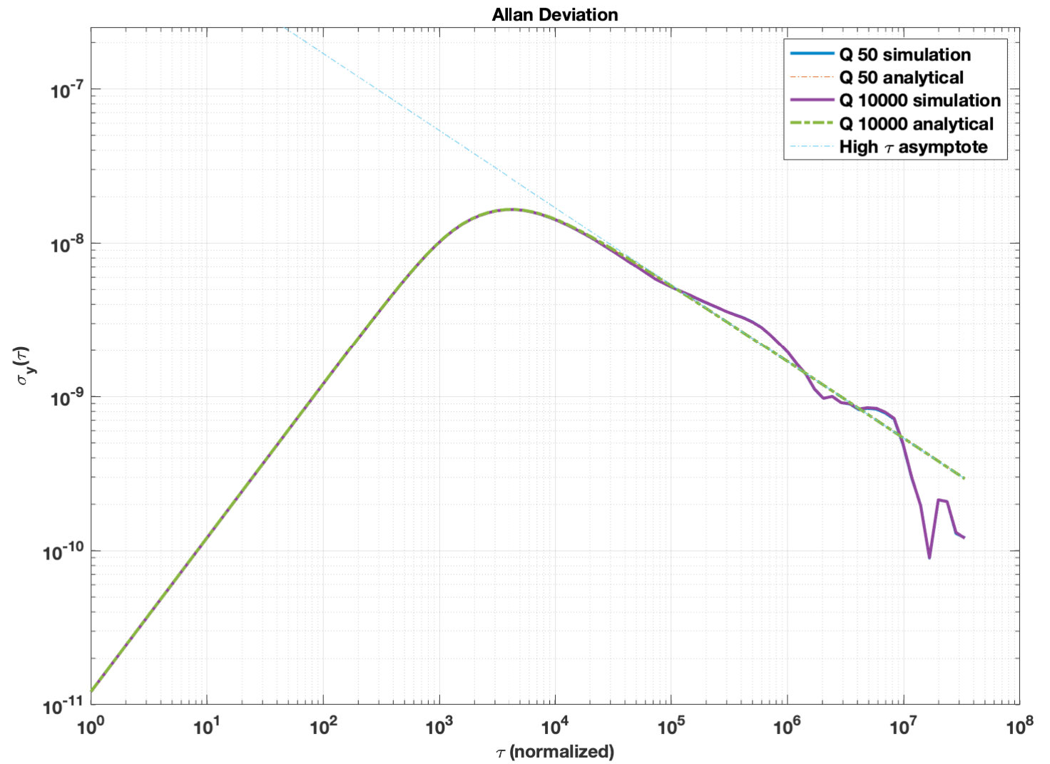 Figure 1
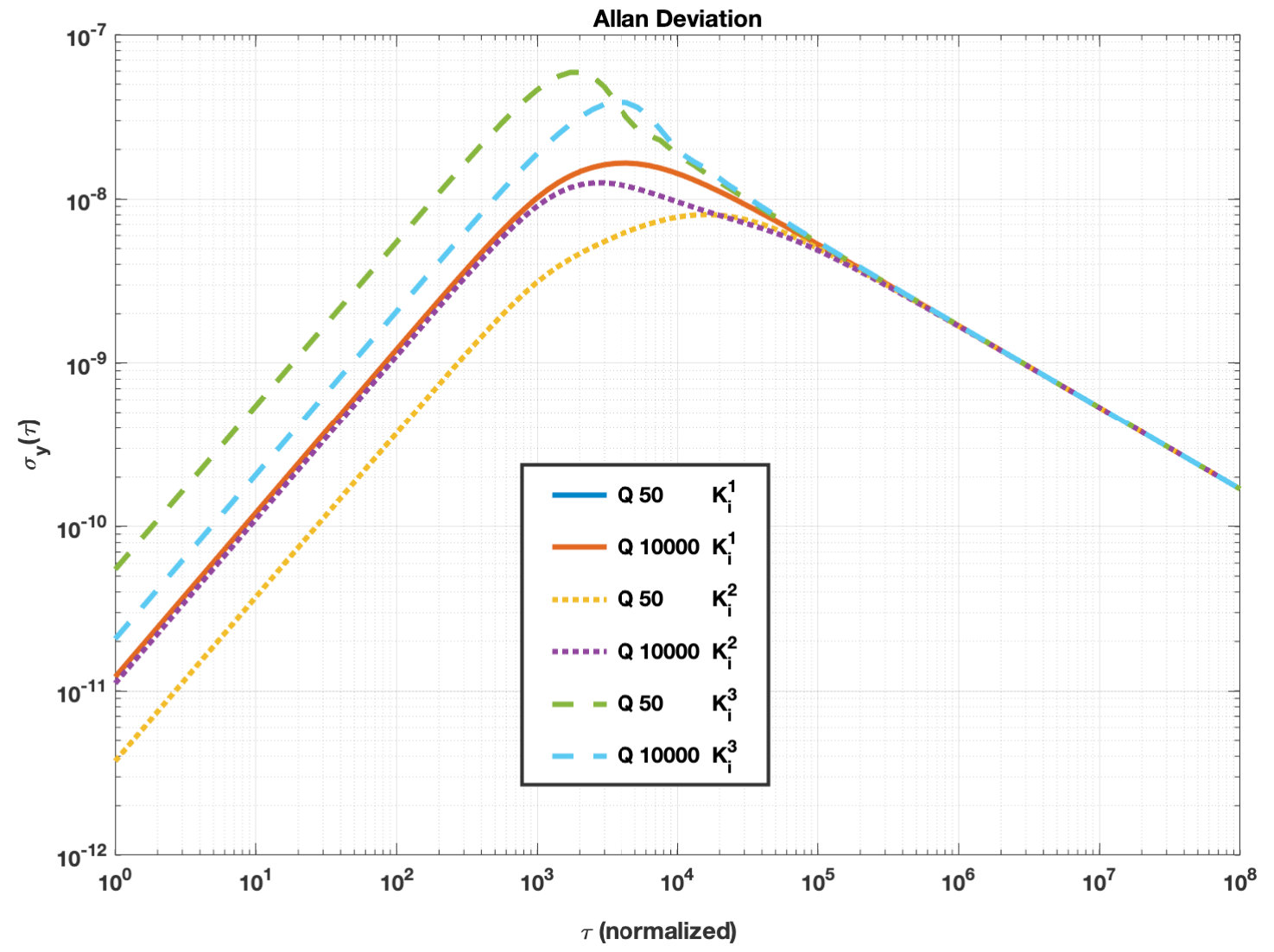 Figure 2
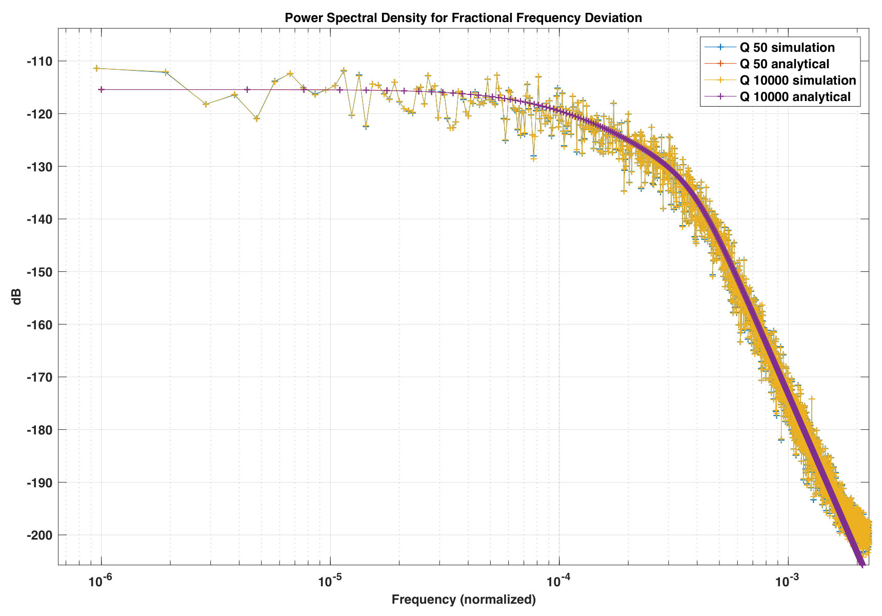 Figure 3
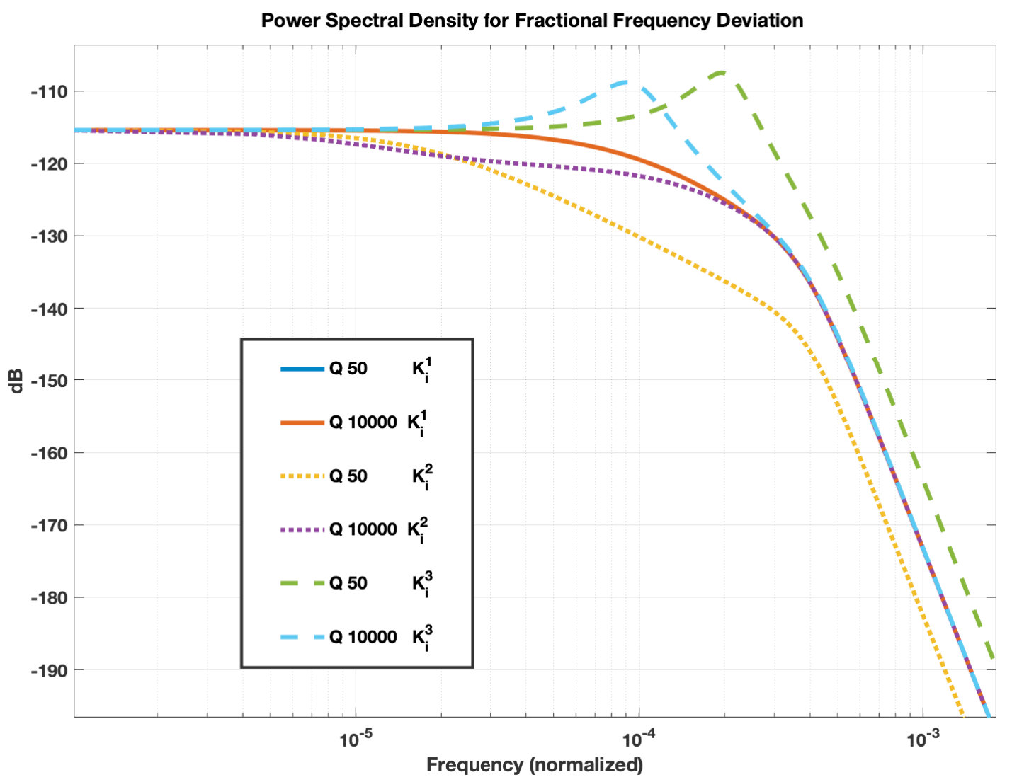 Figure 4
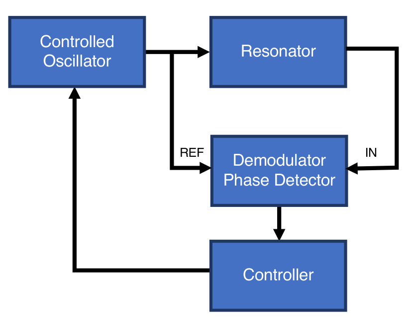 Figure 5
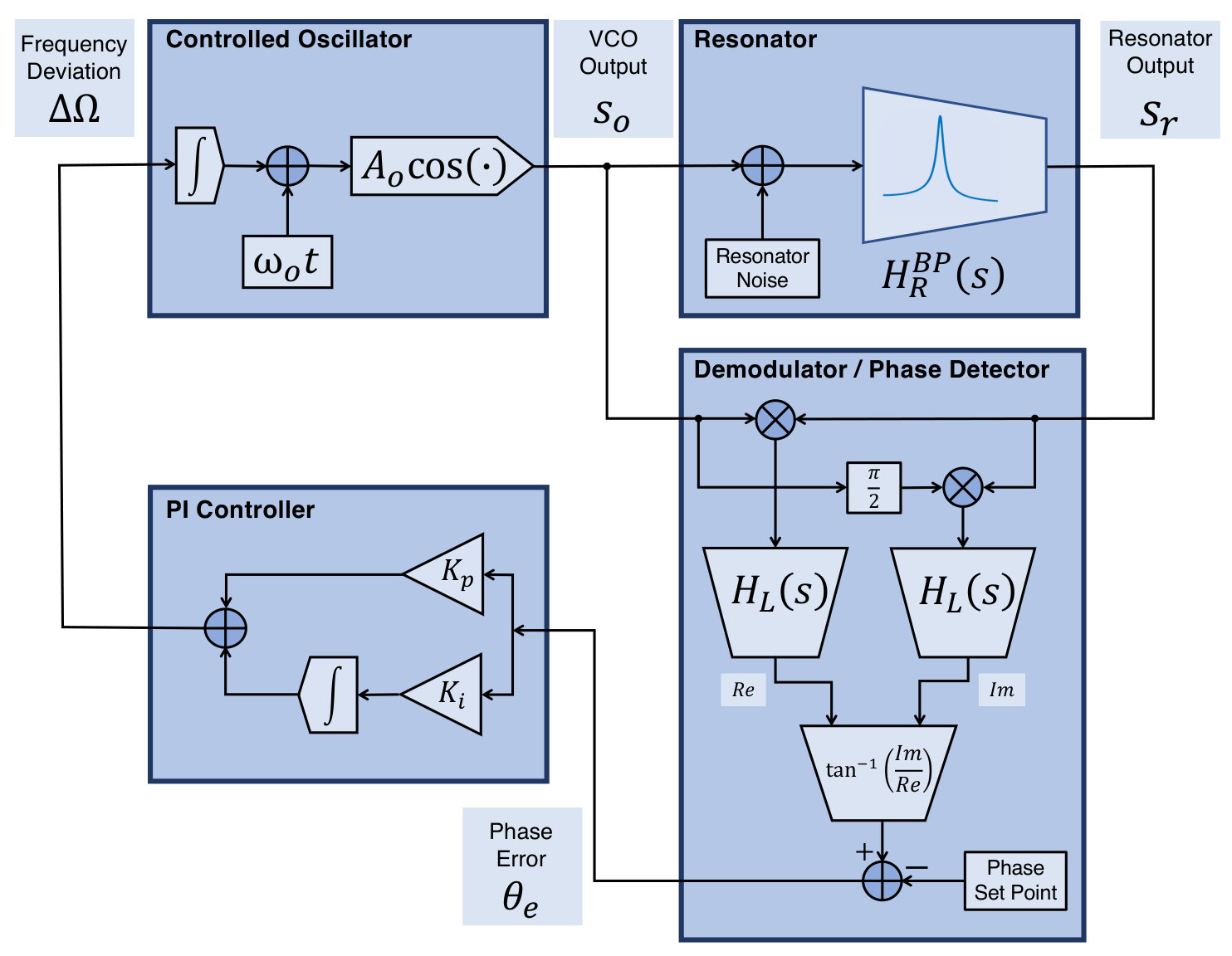 Figure 6
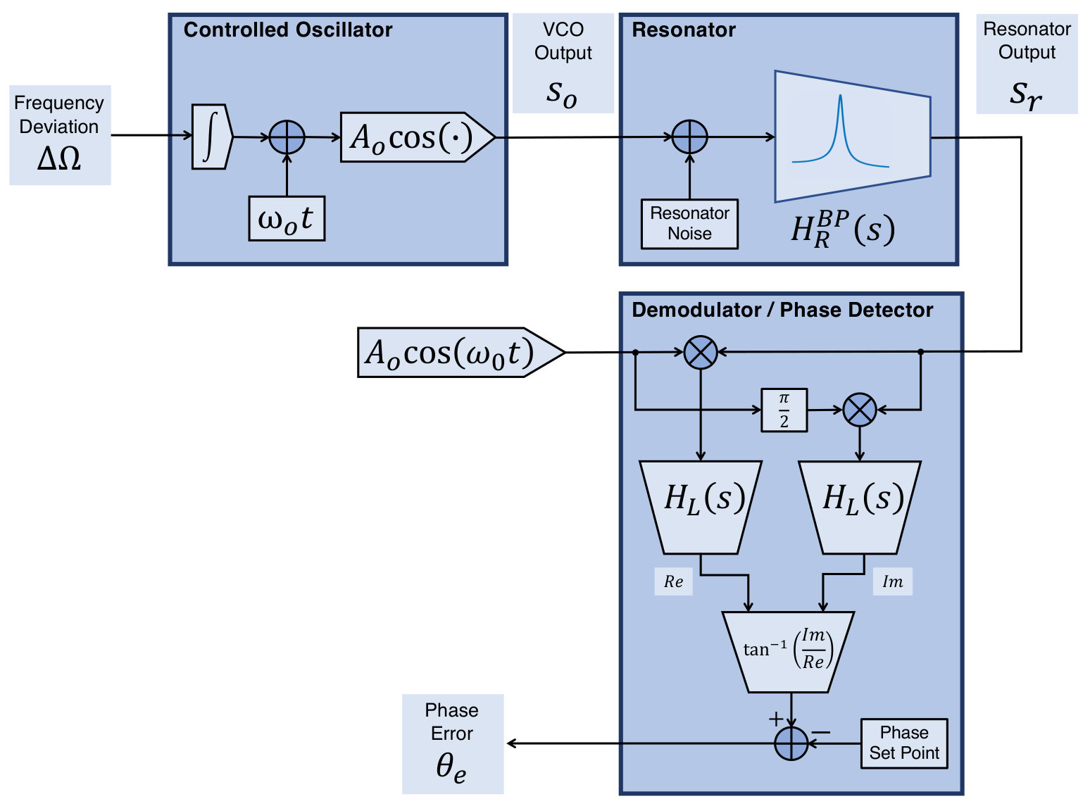 Figure 7
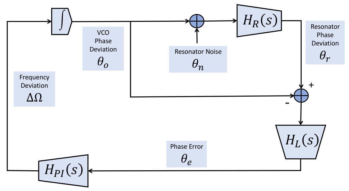 Figure 8
Peer Reviews
No public reviews on file for this paper yet. If you reviewed it on a platform where reviews are public (OpenReview, ICLR, NeurIPS, ICML), you can paste yours below so the community can read it here.
Videos
No videos yet. Explain this paper in a talk, walkthrough, or lecture? Add one.
Phase-Locked Loop based Resonant Sensors:
A Rigorous Theory and General Analysis Framework for
Deciphering Fundamental Sensitivity Limitations due to Noise
Alper Demir
Koç University, Istanbul, Turkey
M. Selim Hanay
Bilkent University, Ankara, Turkey
Abstract
Nanomechanical resonators are used in building ultra-sensitive mass and force sensors. In a widely used resonator based sensing paradigm, each modal resonance frequency is tracked with a phase-locked loop (PLL) based system. There is great interest in deciphering the fundamental sensitivity limitations due to inherent noise and fluctuations in PLL based resonant sensors to improve their performance. In this paper, we present a precise, first-principles based theory for the analysis of PLL based resonator tracking systems. Based on this theory, we develop a general, rigorously-derived noise analysis framework for PLL based sensors. We apply this framework to a setting where the sensor performance is mainly limited by the thermomechanical noise of the nanomechanical resonator. The results that are deduced through our analysis framework are in complete agreement with the ones we obtain from extensive, carefully run stochastic simulations of a PLL based sensor system. We compare the conclusions we derive with the recent results in the literature. Our theory and analysis framework can be used in assessing PLL based sensor performance with other sources of noise, e.g., from the electronic components, actuation and sensing mechanisms, and due to the signal generator, as well as for a variety of PLL based sensor configurations such as multi-mode and nonlinear sensing.
Index Terms:
nano-mechanical sensor, phase-locked loop, thermo-mechanical noise, phase noise, Allan deviation.
I Introduction
State-of-the-art nano-mechanical sensors are extremely sensitive, achieving yoctogram and single-protein resolutions in inertial mass sensing, thanks to their ever diminishing size and high quality factors [1, 2, 3]. Currently, there are two main architectures in use for resonant sensors: (i) Self-sustaining autonomous oscillator, in which a nano-mechanical resonator is used as the frequency selective element in a classic feedback oscillator configuration, with an amplifier and a delay line in the loop [4, 5]. (ii) Phase-locked loop (PLL) configuration that tracks the nano-mechanical resonance frequency by driving the resonator with a voltage/numerically-controlled oscillator which is locked to the resonance. Both architectures have their advantages and shortcomings. However, the accuracy of all NEMS sensors is limited by the inherent fluctuations and noise in the mechanical, electrical and/or optical domains [6, 7, 8, 9], depending on the particular sensing and actuation mechanisms used. Thus, there is great interest in first understanding the fundamental sensitivity limitations due to noise, and then improving the sensor performance [6, 7, 8, 9, 10, 11, 12, 13, 14].
Recently, Roy et al. [14] put forward an idea that is diametrically opposed to the current understanding on how to improve NEMS sensor performance. They proposed that one can achieve much better sensitivities by increasing damping in the resonator, i.e., with resonators that have much lower quality factors. They offer a two-part argument as to how this improvement can be obtained. In the first part, they point out that nano-mechanical resonators with lower quality factors can be driven harder before Duffing nonlinearity kicks in. Higher drive strength in conjunction with larger damping turns the inherent thermo-mechanical noise of the resonator into the dominant source of noise, masking other sources of noise, and enables operation at a higher signal-to-noise-ratio (SNR). Roy et al. adjust the drive strength in such a way so that SNR is inversely proportional to the quality factor , thus operating at the onset of Duffing nonlinearity. This first part of their proposal makes perfect sense. In the second part, Roy et al. claim that, with , one in fact obtains a noise performance that is much better than the expected with a PLL based architecture at a lower . Their explanation regarding as to how this improvement arises for low is based on a revelation that the phase noise spectrum flattens at low frequencies, as opposed to the usual approximation that is commonly employed in high cases. We believe that this second part of their claim warrants further investigation.
In this paper, we get to the bottom of this issue. We investigate in detail whether one can obtain better performance with larger damping in a PLL based sensor. Our conclusion is in the negative. We arrive at this result by developing a first-principles based noise analysis framework for PLL based sensor architectures, where each step and approximation is rigorously justified. The PLL system we consider is shown in Figure 1 as a block diagram, with details shown in Figure 2. We apply our analysis framework to the case considered by Roy et al.. We precisely characterize the performance of a PLL based sensor when the dominant source of noise is the inherent thermo-mechanical noise of the resonator. We perform the noise analysis for different values and feedback parameters. Moreover, our analysis framework is much more general. It can be used to assess the performance of PLL based NEMS sensors with other sources of noise, e.g., from the amplifiers, actuation and sensing mechanisms, and due to the signal generator, as well as for a variety of PLL based sensor configurations such as multi-mode [3] and nonlinear nano-mechanical [15] sensing. Furthermore, the theory we develop is not specific to nanomechanical resonators, it may be used for resonant sensors in other domains, for instance ones that are based on microwave resonators [16].
Our analysis framework does employ some approximations, and is based on some assumptions. Even though all of these are stated very clearly and justified rigorously in our development, we go further in order to verify our theoretical results. We report the results of extensive, carefully conceived stochastic simulations of the PLL system. The simulator does not employ any of the mentioned approximations and assumptions, and is based on realistic, detailed, full models of the system components. The system is simulated with full, high-frequency, nonlinear and time-varying models for the resonator and the demodulator as shown in Figure 2. The simulator is based on the solution of coupled differential equations that are solved using an appropriate numerical technique based on time-discretization. The time step of the simulation is set to be a small fraction () of the period of the high-frequency signal at the output of the resonator. The thermomechanical noise of the resonator is introduced into the simulation using a random number generator. The time series and waveform data produced by the simulation is post-processed for estimating the spectral densities of the signals of interest, as well as in order to compute the Allan Deviation for the frequency tracking performance of the closed-loop system. The results we obtain with the simulator are in complete agreement with the ones deduced via our analysis framework.
The outline of the paper is as follows. We present the models used for the PLL components in Section II. The theoretical development of our analysis framework is in Section III. The results obtained from our theory are verified against the ones obtained with the simulator in Section IV. Conclusions are stated in Section V. Three appendices provide derivations and details, regarding thermo-mechanical resonator noise, spectral characterization and filtering of cyclo-stationary random processes, and Allan Variance, in order to make the paper as self-contained as possible.
II PLL Component Models
II-A Resonator
We consider a resonator that is modeled as a damped harmonic oscillator as follows [17]
[TABLE]
where is the displacement, is the mass, represents a force excitation, is the resonance frequency, and the damping rate is given by
[TABLE]
where is the quality factor. The damping rate determines the line-width of the resonator’s frequency response (from input to output ), which is given by
[TABLE]
Based on the fluctuation–dissipation theorem of statistical thermodynamics, the thermo-mechanical noise of the resonator can be modeled as a white noise source (input-referred, at the input of the resonator as in Figure 2) with a (two-sided) spectral density given by [7]
[TABLE]
where is Boltzmann’s constant, and is temperature (in Kelvins). With this noise source as the only input to the resonator, the mean kinetic energy of the resonator can be computed as follows
[TABLE]
where denotes the probabilistic expectation operator. The expectation above can be computed using the Wiener–Khinchin theorem as below
[TABLE]
where is the power spectral density (PSD) of the resonator displacement , which can be computed with
[TABLE]
where . The integral in (6) can be evaluated, as shown in Appendix A, to yield
[TABLE]
consistent with the equipartition theorem of statistical mechanics.
II-B Demodulator
The demodulator shown in Figure 2 performs essentially as a phase (difference) detector. The controlled oscillator output and the resonator output can be expressed as
[TABLE]
We can express the operations in the in-phase (real) and quadrature (imaginary) arms of the demodulator in a compact manner using complex arithmetic as follows. We first express the resonator output as
[TABLE]
Then, the signals at the output(s) of the multipliers in the demodulator are the real and imaginary parts of
[TABLE]
We next assume that the low-pass filters in the demodulator (shown as ) block the high-frequency, second term and pass the low-frequency, first term above. Thus, the outputs of the filters are given by (the real/imaginary parts of)
[TABLE]
Finally, the output of the block is then simply the phase difference between the resonator output and the control oscillator signal, expressed as
[TABLE]
where we assume that and is a low-frequency signal. In the actual model of the system, we do take into account the non-ideal nature of the low-pass filter by using a practical filter. The attenuation of the high-frequency component in (11) by a practical is in fact quite good due to the large frequency separation, whereas the low-frequency component does get modified by the filter, which we take into account in the analytical theory we develop further below. The phase set point in the demodulator is needed in order to keep the resonator at its resonance, as we show later.
II-C Controller
We use a simple PI controller, as shown in Figure 2, with a transfer function
[TABLE]
We discuss later how to choose the controller parameters and . The input to the controller is the phase error signal from the demodulator (phase difference detector) and the controller output is fed to the controlled oscillator, simply determining its frequency deviation from the nominal value .
II-D Controlled oscillator
The controlled oscillator is an essential component of the PLL. In an all-analog PLL system, it would be instantiated as a high precision analog voltage-controlled oscillator (VCO), typically including a crystal as a time reference. In PLL tracking systems for NEMS applications, lock-in amplifiers (LIA) are routinely employed. In recent LIA based systems, the controlled oscillator is in fact digitally implemented on a configurable DSP/FPGA chip, as what is called a numerically controlled oscillator (NCO). The timing/frequency precision of the NCO is then determined by the time base of the DSP/FPGA, which may be locked to an external atomic reference. For the VCO/NCO, we will use a simple model as follows for its output
[TABLE]
where the frequency deviation is the control signal produced by the PI controller.
Due to the high precision of the VCO or the time base of the NCO, we will assume that the phase noise contribution of the controlled oscillator is negligible. However, both the theory and the simulator that we have developed can be very easily modified to include the phase noise contribution from the VCO/NCO, as well as noise from other components, such as the electronic amplifiers, the actuators and sensors that convert signals between the electrical and the mechanical domain. Our main goal in this paper is to decipher the fundamental sensitivity limitation due to resonator noise.
III Theory
III-A Baseband equivalent phase domain model of the resonator
The PLL based tracking system shown in Figure 2 contains signals with widely varying frequencies, as well as in different domains. The outputs of the NCO and the resonator are at a high frequency, at around the resonance frequency of the resonator. On the other hand, the phase error signal at the output of the phase detector and the frequency deviation at the output of the controller are low-frequency signals, at frequencies below the PLL bandwidth. The frequency separation between these high and low frequency signals is typically at least four orders of magnitude. The signal of interest is the frequency deviation at the input of the NCO, since that is what one uses in a typical sensing setup in order to track the resonance frequency deviations. The challenge in analyzing the PLL system is then to accurately characterize the slow dynamics of the frequency deviation signal while capturing the impact of the fast dynamics of the NCO and the resonator in a correct manner. In order to accomplish this in a simple and tractable manner, we will first develop a base-band (low-frequency) equivalent model of the NCO-resonator-demodulator signal chain. The input and output of this chain of blocks are both low-frequency signals, whereas there is first low-to-high and then high-to-low frequency translation of signals along the chain, and also a nonlinear operation at the very end. This makes this composite system, the cascade connection of NCO-resonator-demodulator, both nonlinear and time-varying. Fortunately, we will be able to develop a simple, linear and time-invariant model for this cascade that is quite accurate, which is verified against numerical simulations of the full, nonlinear and time-varying system.
In order to develop this simple model, we consider the open-loop NCO-resonator-demodulator chain shown in Figure 3. We note that, in constructing the open-loop model, not only we have disconnected the main PLL loop but also we no longer feed the second demodulator input with the signal from the NCO. Instead, the second demodulator input is simply set to a sinusoidal signal at a constant frequency. In the final simplified model we will construct, we will take into account the fact that the second demodulator input is in fact set to the NCO output. In the development below, we set the resonator noise to zero and first construct a simplified model for the deterministic dynamics. We will then also consider the resonator noise and include it in the final model.
We now walk through the chain, from the input (frequency deviation) to the output (phase error) . The phase deviation of the NCO, is related to the frequency deviation simply with an integral
[TABLE]
The output of the NCO is then given by
[TABLE]
The operation above constitutes a low-to-high frequency translation, from to . We next consider only the first term on the second line of (17). As discussed in Section II-B, the signal that will arise from the second term down the resonator-demodulator signal chain will be eventually blocked by the low-pass filter . Then, the input to the resonator is given by
[TABLE]
In order to compute the effect of the resonator on the signal, we now transform to frequency domain, by computing the Laplace transform (bilateral) of above:
[TABLE]
where is
[TABLE]
While is a high-frequency, pass-band signal with its power concentrated around in the frequency domain, is a base-band, low-frequency signal with its power concentrated around zero frequency. When the PLL is tracking the resonance of the resonator, the NCO center frequency would be nominally equal to the resonant frequency of the resonator. If there is any resonance frequency shift in the resonator, PLL would compensate for this by adjusting the frequency deviation , and accordingly the phase deviation , of the NCO. Thus, without loss of generality, we assume as we proceed below.
We now compute the output of the resonator (in the frequency domain) with its input as in (19)
[TABLE]
where is the resonator transfer function in (3). Nominally, has a pass-band characteristics centered around in the frequency domain. Thus, with the input as a pass-band signal centered around the same frequency, so is the output . Hence, we have
[TABLE]
and
[TABLE]
where is a base-band, low-frequency signal with its power concentrated around zero frequency. Combining (19), (21) and (23), we obtain
[TABLE]
We define
[TABLE]
as the base-band equivalent transfer function of the resonator, which is given by
[TABLE]
where we used (3) and (25), and substituted and . can be used as a base-band equivalent model for the resonator. However, an approximate (first-order) form for (second-order) that we derive below simplifies the rest of our derivations considerably.
We manipulate (26) (by combining the first and third terms in the denominator of the dependent part) to obtain
[TABLE]
We note that in (27) above is small when compared with . This is due to the frequency shift operation represented by (25). In the pass-band model of the resonator represented by , we have , whereas in the base-band equivalent model represented by , we have . We then assume that in (27) and use the following approximations due to low-frequency, base-band nature of
[TABLE]
The above can be interpreted as a sort of high- approximation, but our goal is to develop a theory that is valid even for low- resonators. We verify later against simulations (which do not incorporate any approximations) that the base-band resonator model based on the above approximations remains accurate for a that is as low as 10. With the above approximations, can be simplified as follows
[TABLE]
Finally, can be represented as a Laplace transform:
[TABLE]
We define the resonator time constant with
[TABLE]
and obtain
[TABLE]
The above is essentially a first-order, one-pole, low-pass transfer function, with a DC gain and an extra phase shift. If the input to the resonator is a pure tone at the resonance frequency (corresponding to in (32)), then the steady-state output (also a pure tone at the same frequency) will have a phase shift with respect to the input.
We note that a resonator model as in (32) was derived in [18]. However, our treatment above based on the use of the base-band equivalent transfer function concept streamlines the model development process and reveals the exact nature of the approximations involved. The base-band equivalent representation for band-pass signals is commonly used in the analysis of communication systems [19]. This technique is similar to the ones used in other disciplines, known as complex amplitude representation for slow dynamics [10], and slowly varying envelope approximation [20].
Next, we move along the signal chain and characterize the impact of the demodulator. The demodulator features high-to-low frequency translation, undoing the low-to-high frequency translation that was done by the NCO. That is, the signals at the output(s) of the multipliers in the demodulator, in Figure 3, are the real and imaginary parts of
[TABLE]
We substitute (22) into the above equation to obtain
[TABLE]
That is, the demodulator simply extracts the base-band equivalent, low-frequency, complex-valued resonator output . However, this signal is further processed in the demodulator through the low-pass filter denoted by . This filter will nominally not modify . However, it is required in order to remove the high-frequency signals (at the outputs of the multipliers) that will arise from the second term in (17), which we have ignored upfront.
The phase angle of the complex-valued output of the low-pass filters is produced with the block in the demodulator. Let the inputs to the block be the (real and imaginary parts of)
[TABLE]
where is the possibly time-varying amplitude, and is the phase. The output of the block is simply the phase . Then, we have
[TABLE]
Thus, we have obtained a compact and simple model for the entire signal chain from the phase deviation of the NCO to the phase error , output of the phase detector. In doing so, we were able to capture everything with low-frequency signals, in a base-band equivalent manner. That is, the model in (36) does not have any explicit frequency translation operations, making it time-invariant. However, this model is still nonlinear due to the phase-to-complex conversion, i.e., , in the NCO, and the complex-to-phase conversion, i.e., , in the demodulator. Next, we introduce a further approximation in order to obtain a simple, linear and time-invariant model for the entire signal chain from to .
We first observe that the block makes any scaling or DC gain factor up to that point along the signal chain irrelevant, i.e., the factor in (20), the DC gain in (32), any DC gain in , and the factor in (34) are all immaterial for the final output of the demodulator. The final operation in the demodulator subtracts the phase set point from the computed phase, and is set to due to the phase shift in (32) due to the resonator. (Please note that the phase set point is, not related to, and distinct from the phase shift applied to the NCO signal for the quadrature arm of the demodulator.) Here, we assume that does not introduce any extra phase shift for (complex-valued) DC signals. In this case, if the phase deviation of the NCO is time-invariant, set to a constant as , then the final output of the demodulator, i.e., the phase error , is simply equal to this constant phase . Thus, we remove all scaling factors, DC gains, as well as the phase shift in resonator, from the signal path, without changing the final phase error output of the demodulator. We define
[TABLE]
which was obtained from (32) by removing the DC gain and the phase shift. We assume that the low-pass filter has a DC gain of 1 and introduces no phase shift for (complex-valued) DC signals, i.e., . We then modify (36) to obtain
[TABLE]
We next assume that the phase deviation is small enough so that we can use the following approximation
[TABLE]
The constant DC factor 1 above (real part) will go through and unmodified since , whereas will be modified by the dynamics of these filters, producing
[TABLE]
where
[TABLE]
Thus, the phase error (ignoring phase set point) can be computed with
[TABLE]
Since , we have
[TABLE]
Thus, we have obtained a simple, linear and time-invariant model for the entire signal chain from the frequency deviation to the phase error .
In deriving the model above, we assumed that the second demodulator input is simply set to , as in the open-loop model in Figure 3. In the closed-loop PLL, this input is in fact set to the output of the NCO, making the demodulator effectively a phase difference detector between the resonator and the NCO outputs. We now construct a base-band equivalent, phase domain model for the closed-loop PLL, as shown in Figure 4, by taking this into account. In this model, the PI controller is represented as a transfer function given in (14). We have verified all of the approximations we have performed in deriving the phase domain model against simulations of the full nonlinear, time-varying system model. However, we emphasize that, for the model in Figure 4 to be valid, the base-band equivalent resonator transfer function and the demodulator low-pass filter transfer function need to satisfy .
III-B Baseband equivalent noise model for the resonator
Having derived a simple model for the deterministic dynamics of the system, we now turn to doing the same for the noise dynamics. We consider the open-loop system in Figure 3 and initially set the NCO output to zero. Thus, the resonator-demodulator chain is driven by only the resonator noise source, modeled as a stationary, white Gaussian random process with a (two-sided) PSD as given in (4). This white noise source is shaped by the resonator, turning into a colored noise process with a pass-band PSD, but still stationary. In the demodulator, it goes through the two mixers (multipliers), turning into cyclo-stationary noise processes [21, 22, 23]. As we will see later, the low-pass filters in the demodulator not only block the high-frequency parts but also stationarize these cyclo-stationary noise processes by removing the high-order cyclo-stationary components [21, 22, 23]. Finally, the noise processes in the in-phase (real) and quadrature (imaginary) arms of the demodulator converge at the nonlinearity, which performs a real/imaginary-to-phase conversion, yielding a phase error noise process at the very end. The phase set point subtraction is a DC operation, and was taken into account as part of the deterministic dynamics of the system considered before. As summarized here, the thermo-mechanical noise of the resonator goes through a nonlinear and time-varying system with inherent frequency translation operations. However, as we did for the deterministic dynamics, we will be able to model the entire noisy dynamics as captured by a much simpler system, where an equivalent stationary noise process passes through base-band equivalent linear and time-invariant filters.
We follow the noise path in Figure 3 starting from the input of the resonator. With the PSD of the noise source at the resonator input as in (4), the noise PSD at the resonator output can be computed as follows
[TABLE]
Next, this pass-band stationary noise process is fed into the two multipliers that generate cyclo-stationary noise, which can not be characterized with a simple PSD. For cyclo-stationary processes, the PSD is a function of two variables, the frequency and time , i.e., , where the dependence is periodic and can be represented with a Fourier series as discussed in Apppendix B [21, 22, 23]. The noise signal at the output of the in-phase (real part) multiplier is given by
[TABLE]
where is the stationary noise signal at the output of the resonator with the PSD in (44). Then, the cyclic spectra of , as shown in Apppendix B, is given by
[TABLE]
The noise signal at the output of the quadrature (imaginary part) multiplier is given by
[TABLE]
It can be easily shown that the cyclic spectra of is
[TABLE]
The cyclo-stationary noise signals and at the outputs of the multipliers are filtered with the low-pass filter . As shown in Apppendix B, this filter stationarizes these cyclo-stationary noise processes, and at the same time removes high-frequency components [22]. The stationary noise signals, and , at the output of these filters have the following PSD
[TABLE]
where is the PSD in (44). We next analyze the noise folding (discussed in Apppendix B) and filtering represented by (49). is a pass-band, two-sided PSD with power concentrated around . Thus, has power concentrated around 0 and , whereas for it is around 0 and . Assuming that is a low-pass filter with an effective bandwidth that is much less than , satisfying , it will remove the noise component at in and the one at in . Then, the only noise components of interest are the ones around 0. We evaluate these components as follows. We first rewrite (44) as below
[TABLE]
and then
[TABLE]
We then assume that and use the following approximations due to the fact that we are interested in the above PSD only at low frequencies
[TABLE]
The above approximations are similar to the ones in (28) that we employed in simplifying the deterministic dynamics. With (52), (51) can be simplified as follows
[TABLE]
We substitute (53) above into (49) to obtain
[TABLE]
We observe that
[TABLE]
with defined as in (37). Thus,
[TABLE]
Final stage in the demodulator is the block, a memoryless nonlinearity. Up till now, we assumed that the resonator-demodulator chain is driven by only the resonator noise source. In order to correctly evaluate the effect of the nonlinear block, we need to also consider the signal input to the resonator that is fed from the NCO output. With NCO output set to
[TABLE]
the deterministic components of the in-phase and quadrature signals at the inputs of the block will be the real and imaginary parts of
[TABLE]
based on (12) and (32). The output of the can be computed as follows
[TABLE]
where and are the noise signals at the inputs of . We observe that the noise signal above is much smaller than the DC signal term . Thus,
[TABLE]
Furthermore, the noise term is also small. Thus, we use the following first-order Taylor’s series expansion
[TABLE]
Hence, we have
[TABLE]
With the subtraction of the phase set point, i.e., at the output of the demodulator, the phase error is given by
[TABLE]
Then, the PSD of can be computed based on (56) and (63):
[TABLE]
We use (31) in (64) and define
[TABLE]
as the PSD of a white, Gaussian noise process . represents the thermo-mechanical noise of the resonator, in an input-referred manner, in the base-band equivalent phase domain model in Figure 4. This noise process goes through two filters, and , as in both (64) and Figure 4, to produce the phase error noise at the output of the demodulator, i.e., the input of the PI controller
III-C PLL noise analysis
Having derived base-band equivalent phase domain models for both the deterministic and noise dynamics of the PLL components, we next proceed with the noise analysis of the closed-loop system based on Figure 4.
The closed-system is governed by the following equation, written directly in the frequency domain, by going around the loop in Figure 4:
[TABLE]
We compute the transfer function from to by solving the loop equation above, and substitute (14) and (37) into the result to obtain
[TABLE]
We manipulate the above expression to obtain
[TABLE]
Due to (16), the transfer function from to the NCO frequency deviation is
[TABLE]
We can then compute the PSD for the frequency deviation of the NCO as follows
[TABLE]
with as given in (65). We note that the transfer function in (68) satisfies
[TABLE]
with an appropriate low-pass filter in the demodulator. That is, represents a low-pass filter, with a bandwidth that is essentially the loop bandwidth for the PLL. With in (65) representing a white spectrum and due to (69), the frequency deviation has the characteristics of band-limited (low-pass filtered) white noise. The phase deviation , the (time) integral of , then has the characteristics of a random walk, albeit not in the form of a standard Wiener process (Brownian motion). However, for longer time scales (larger than the PLL loop time constant) does behave as a standard random walk process. We emphasize here that this random walk aspect of the phase deviation is not arising from the inherent phase noise of the VCO or NCO. We recall that we have set the inherent phase noise of the controlled oscillator to zero, upfront, when we started our analysis. The random walk nature of phase deviation we have derived above is due to the fact the thermo-mechanical noise of the resonator circulates around the loop. One can interpret that the loop dynamics converts the additive, thermo-mechanical noise (in amplitude) of the resonator into phase noise in the NCO. Our analysis above reveals, in a rigorous manner, precisely how this conversion occurs. This resultant phase noise in the NCO ultimately limits the frequency tracking accuracy of the PLL and represents a fundamental limit on the sensitivity of the resonator based sensor system. Based on the model and theory we have developed above, we next precisely characterize the frequency tracking accuracy of the PLL architecture in terms of Allan Deviation.
III-D *Characterizing PLL performance via Allan
Deviation*
Allan Deviation [24, 25, 26] is the standard measure of frequency stability. It is widely used in assessing the sensitivity of resonant sensors. Please see [24, 25, 26] for details on Allan Deviation. Our discussion is based on [24, 25, 26].
We define to be the fractional frequency deviation as follows
[TABLE]
where is the NCO frequency deviation, and is the nominal NCO frequency. The averaged fractional frequency deviation is defined as
[TABLE]
where is the averaging time. The th sample of is given by
[TABLE]
where the sampling interval is chosen to be equal to the averaging time for standard Allan Deviation. Finally, Allan Variance is computed as follows
[TABLE]
where where denotes the probabilistic expectation operator. The Allan Deviation is then
[TABLE]
We note that the above definition implicitly assumes or postulates that is a function of only the averaging time , and is independent of the sampling times represented by and . This is the case when is a (wide-sense) stationary process. This is satisfied in our setting, since the frequency deviation is indeed a stationary process, as the output of a stable, linear and time-invariant system (with transfer function in (68)) with its input set to white, stationary, Gaussian noise .
It can be shown that (as in Appendix C)
[TABLE]
where is the PSD of given by
[TABLE]
due to (71) with in (69). With the transfer function in (68), it is, unfortunately, not possible to evaluate the Allan Variance integral in (76) analytically. However, we can evaluate it numerically in order to compute the Allan Deviation for all values of , for any choice of the low-pass filter and the controller parameters and . We will present results for this numerical evaluation in Section IV. On the other hand, it is really desirable that we have an analytical handle on the frequency tracking accuracy of the PLL system. We next evaluate the integral in (76) analytically, for values of that are larger than the loop time constant, thus computing a high- asymptote for the Allan Deviation of the PLL tracking system. This result will be practically valuable, since the PLL is able to track the frequency deviations of the resonator within its bandwidth, or in other words, at time scales that are longer than the loop time constant. Allan Deviation for values of larger than the loop time constant is important from a practical point of view. Frequency deviations that occur faster than the loop time constant are attenuated by the loop dynamics, rendering the PLL tracking system not useful at short time scales.
The high- asymptote for in (76) can be computed by approximating the low-pass PSD with its value at zero (low) frequency, i.e., with
[TABLE]
where we used (69) and (70), with as a constant function of as given in (65). Next, we substitute (78) in (76) and evaluate the integral to obtain
[TABLE]
We note that above is the resonator time constant defined by (31), whereas is the averaging time used in the definition of Allan Variance. The above result for is valid for large , larger than the loop time constant. We use (65) and (31) in (79):
[TABLE]
The factor (that multiplies ) above is expressed in terms of the resonator parameters , , , Boltzmann’s constant , temperature , and the amplitude of the signal that drives the resonator. We would like to express this factor in terms of a Signal-to-Noise-Ratio (SNR) for the resonator. We define SNR as follows
[TABLE]
In the above, is the input-referred, white (two-sided) PSD of the thermo-mechanical noise of the resonator given in (4). BW is defined as the (one-sided, hence the factor of 2) noise bandwidth. BW is typically set to the bandwidth of the low-pass filters in the demodulator. Alternatively, it could be set to the PLL loop bandwidth. The particular choice for BW simply affects the SNR definition, there is nothing fundamental about it. We note the following relationship for the product of and SNR:
[TABLE]
Allan Variance in (80) can be expressed in terms of the product :
[TABLE]
and Allan Deviation is
[TABLE]
The high- approximations above for Allan Variance and Deviation with and dependence represent random walk phase noise [25, 26]. Indeed, for time scales larger than the loop time constant, the resulting phase deviation, arising from the thermo-mechanical noise of the resonator and the loop dynamics, has a random walk nature. As we will see in Section IV, Allan Deviation will have a different dependence on for shorter time scales, however, still with the same front (scaling) factor that has a form. We note that the result in (84), valid for high-, is independent of the loop and controller parameters (apart from an indirect dependence on them through BW definition) such as and and the particular choice for the filter transfer function . On the other hand, these parameters do determine the loop bandwidth and time constant, and how Allan Deviation changes with for short time scales within the loop time constant. However, we emphasize, the scaling factor applies in this case as well.
IV Results versus Simulations
In developing the theory in Section III, we used several approximations and assumptions:
We assumed that the resonator output signal is a strictly band-limited band-pass signal, and that the low-pass filters in the demodulator/phase detector completely remove the high frequency signal and noise components produced by the multipliers. This allowed us to develop simpler, base-band equivalent models for the resonator and the phase detector.
The base-band equivalent transfer function for the resonator and the thermo-mechanical noise PSD were approximated as in (29) and (53). This allowed us to model the resonator with a one-pole low-pass transfer function in a base-band equivalent manner.
We have used a linear(ized) model for the nonlinearity for both the deterministic and noisy dynamics of the PLL, as in (39), (40) and (61). This allowed us to derive a phase domain, in addition to base-band equivalent, model for the loop dynamics.
In deriving the deterministic and noise models for the resonator and the phase detector, we used the open-loop setting in Figure 3, where the second demodulator input was set to . In the closed-loop system, this input comes from the NCO and is equal to , including the phase deviation . In the closed-loop phase domain model in Figure 3, we took this into account by feeding the second demodulator input from the NCO output. However, the base-band equivalent resonator noise model was derived in Section III-B based on the assumption that the second demodulator input does not have any phase deviation. This simplified the noise model derivation considerably.
Even though the above assumptions and approximations are well founded and justified, we still would like to verify them. We do this by comparing our analytical results against the ones obtained from extensive, carefully crafted and run, time-domain stochastic simulations of the PLL system. In these simulations, none of the above assumptions and approximations are used. The system is simulated with full, high-frequency, nonlinear and time-varying models for the resonator and the demodulator as shown in Figure 2.
We next provide details and describe specific choices for the resonator and system parameters. The PLL bandwidth is typically set to a small fraction of the resonance frequency and is limited by the capabilities of the loop components such as the LIA. We choose the controller parameters and as follows, as suggested in [18],
[TABLE]
where is the desired loop bandwidth. If we substitute (85) into (68), a pole-zero cancellation occurs in the transfer function, as shown in [18], and simplifies to
[TABLE]
The bandwidth of the filters in demodulator are set to be larger than the desired loop bandwidth , implying
[TABLE]
Hence, we have
[TABLE]
Thus, the loop bandwidth is indeed set to be , with an effective one-pole, first-order loop dynamics. Resonator and system parameters are chosen as follows, similar to the choices in [14]. PLL bandwidth is set as
[TABLE]
Hence, the loop time-constant is equal to periods of the high-frequency signal at the output of the resonator. The low-pass filters in the demodulator are chosen as th order Butterworth filters with pass-band edge frequency set to
[TABLE]
We define the dynamic range DR for the resonator in terms of SNR:
[TABLE]
We present results for two cases, a low quality factor, , and a high one, , with the same resonance frequency. In order to compare these two cases at the onset of Duffing nonlinearity, we adjust the drive strength for the resonator in such a way so that
[TABLE]
as suggested in [14]. For , we choose . For then, we set
[TABLE]
in accordance with (90). We choose BW in the SNR definition same as the bandwidth of the filters in the demodulator
[TABLE]
We set the duration of the simulation to be periods of the high-frequency signal at the output of the resonator, which is equal to loop time constants.
In Figure 5, we present results obtained for Allan Deviation, for and , based on both the analytical derivations in Section III and the simulations. For the analytical results presented in Figure 5, the Allan Variance integral in (76) was evaluated numerically. For the results based on simulation, Allan Variance was estimated from simulation time-series data using the overlapping Allan variance estimator [26]. The axis in Figure 5 is normalized, i.e., shows the number of cycles of the resonator output signal. We note that the high- approximation that was derived in (84) indeed coincides with the results in Figure 5 for , forming a high- asymptote. The loop time-constant is (normalized).
In Figure 6, we present results obtained for the PSD of fractional frequency deviation defined by (71). This figure contains results for and , based on both the analytical derivations in Section III and the simulations. The analytical results presented in Figure 6 were obtained by simply evaluating (77), (69) and (68). The results based on simulations were obtained via spectral estimation from simulation time-series data using Welch’s method [27]. The frequency axis in Figure 6 is normalized with the resonance frequency. We note that the PSD of frequency deviation has a Lorentzian shape, for low frequencies and up to and exceeding the loop bandwidth, as predicted by (88). For larger frequencies on the other hand, PSD exhibits a faster roll-off due to the effect of the high-order low-pass filters in the demodulator.
We note that there is excellent agreement between the analytical results and the ones obtained from simulations, both for Allan Deviation and the spectrum of the frequency deviation. Discrepancies at larger values of are expected for Allan Deviation, due to the inaccuracy of Allan Variance estimation for large values of from time-limited simulation data. The agreement at low values of , below and exceeding the loop time constant, is excellent.
It is noteworthy that the simulation results perfectly agree with the analytical results derived in Section III: If SNR and are related as in (90), the Allan Deviation is independent of for all values of . The results presented in Figure 5 and Figure 6 for the two values fall on top of each other. This correspondence is exact, due to the scaling factor in (84) and the choice for the controller parameters in (85). This particular choice for the controller parameters and in (85) is unique in the sense that it results in a pole-zero cancellation [18] in the transfer function , making its poles and zeros independent of or the resonator time constant . (We note that, in this case, the poles/zeros are independent of , but still appears in a front factor in .) Thus, Allan Deviation is then independent of for all values of , when SNR is adjusted so as to hold the product constant. On the other hand, if the controller parameters and are not chosen as in (85), or if another type of controller is used, then the Allan Deviation will not be independent of for all values of , even when is held constant. However, we emphasize, the high- asymptote (for values of larger than the loop time constant) will always be given by (84), i.e., independent of with constant . The controller parameters and the particular controller design has an effect on the Allan Deviation only for low values of , at or below the loop time constant, which is not significant from a practical point of view, since the PLL system is useful in tracking frequency deviations only at time scales longer than the loop time constant. In order to illustrate this, we show in Figure 7, the Allan Deviation (based on the theory presented in the paper) for three different choices for :
[TABLE]
Above, is the same as in (85), and all other system and resonator parameters were chosen as described before. We observe in Figure 7 that, for , lower yields seemingly better performance for low values of . This is due to the fact that the transfer function has a smaller effective bandwidth for the particular placement of its poles and zeros for the lower case. However, this also means that the PLL will be attenuating the frequency shifts induced by events of interest, e.g., addition of mass, more severely, rendering it not useful for sensing at time scales where the Allan Deviation for lower is smaller than the case for higher . This can be observed in Figure 8 (based on the theory presented in the paper), where PSD of fractional frequency deviation is shown for both and , for the three values of in (91). We observe in Figures 7 and 8 that the lower Allan Deviation is accompanied with more severe attenuation of frequency deviation. With the PLL architecture considered, one can not improve performance at practically relevant time scales (corresponding to the high- asymptote in Figure 7 where all curves coincide) by simply optimizing the controller parameters. The controller parameter choice in (85) in fact strikes a good balance between Allan Deviation and the attenuation of frequency deviations. Since the frequency deviation PSD in this case is maximally flat [18] below the low bandwidth, the step response of the PLL system will not exhibit any ringing and overshoots.
The results we have derived and reported here are in stark contrast to the theory and results presented in [14]. The theory presented in [14] does not consider the closed-loop dynamics of the PLL tracking system. The flattening of the phase spectrum at low frequencies is the basis of the claim in [14] that the sensor performance can be improved with larger damping. Our theory and results show that there is no such flattening of the phase noise spectrum under feedback in a PLL. In fact, as phase deviation is simply the integral of the frequency deviation , and since has a Lorentzian PSD, the phase spectrum (given by times the spectrum of ) does not flatten at low frequencies. On the contrary, the phase spectrum keeps increasing as frequency is lowered, a signature of nonstationary and random walk phase noise. In [14], it is suggested that one can circumvent random walk phase noise in a PLL based system if a high precision NCO/VCO is used. Our theory suggests otherwise. A high precision NCO/VCO will not produce (or produce very little) random walk phase noise arising from its own, internal noise sources, provided that it is controlled with a constant, noiseless frequency control input. However, in the context of a PLL, the frequency control input is noisy, due to unavoidable noise from other sources (resonator, amplifiers, etc.) circulating around the loop and shaped by the loop dynamics. This is a fundamental aspect of PLL operation.
V Conclusions
We have presented a theory and noise analysis framework, and an associated simulator, for PLL based resonant sensors, which is useful in deciphering the fundamental limitations and understanding basic trade-offs due to inherent noise and fluctuations arising from a number of sources. The framework we have described enables a firm analytical handle on the problem, but without forfeiting rigor and precision. In this paper, we considered a setting where the dominant source of noise is the thermo-mechanical noise of the resonator. In future work, we will extend the analysis framework and the simulator to take into account other types of noise and nonideal dynamics in the resonator [6], electronic amplifier and instrumentation noise, fluctuations that arise from the actuation and sensing mechanisms in the mechanical, electrical and optical domains, non-negligible phase noise of the controlled oscillator (signal generator), quantization noise in digital (DSP/FPGA) realizations of some PLL loop components. Furthermore, we will also develop extensions so that the analysis framework can be applied to a variety of PLL based sensor configurations, such as multi-mode mass spectrometry with multiple PLLs [3], and nonlinear nano-mechanical trajectory-locked loop (TLL) [15] based sensing. Even though we have shown that lowering the quality factor of the resonator does not result in the claimed performance improvement, one may be able to obtain better performance by optimizing the controller and the filters in the demodulator in the presence of a variety of noise sources, that we plan to investigate in the near future using the proposed analysis framework.
Appendix A Thermo-mechanical Noise
In this appendix, we evaluate the integral in (6), which is reproduced here for convenience:
[TABLE]
where
[TABLE]
with
[TABLE]
and
[TABLE]
Please see [28] where a power-law noise source driving a parallel RLC circuit is considered. The below treatment is based on [28], with (92) as a special case of the problem considered there.
We substitute (95), (94) and (93) in (92), and manipulate to simplify and obtain
[TABLE]
We substitute (2) into the above and reorganize:
[TABLE]
Next, a new variable of integration is defined as in [28]
[TABLE]
We rewrite the integral in (97) as follows:
[TABLE]
where we used the fact that
[TABLE]
and assumed
[TABLE]
Based on the above, the double-sided integral in (97) was turned into a one-sided one with the new integration variable , since the integrand is an even function of . The final form of the integral in (99) above can be evaluated, by defining [28]
[TABLE]
and using contour integration in the complex plane [28] to yield . Please see [28].
Finally, we have
[TABLE]
Appendix B Spectral Characterizations and Filtering of
Cyclo-Stationary Processes
Please see [21, 22, 23] for details regarding the spectral characterization and filtering of cyclo-stationary random processes. Our treatment below is based on [21, 22, 23].
Let be a zero-mean, stationary Gaussian random process with the auto-correlation function
[TABLE]
where denotes the probabilistic expectation operator. is a function of only , not , due to the stationarity of the process. The PSD of is defined as the Fourier transform of
[TABLE]
Let be a periodic modulating signal. We obtain the modulated signal (random process) from as follows
[TABLE]
The auto-correlation function of is also a (periodic) function of and can be computed as follows
[TABLE]
where
[TABLE]
The PSD of is also a (periodic) function of , in addition to . The dependence can be expanded into a Fourier series [21, 22, 23]
[TABLE]
where are called the cyclic spectra. In (106), the Fourier transform is with respect to the variable . For a stationary process, we have for . In this case, corresponds to the usual PSD for a stationary process [21, 22, 23].
Using (104), (105) and (106), we obtain
[TABLE]
Next, we consider the (low-pass) filtering of with a (linear and time-invariant) filter frequency response [21, 22]. The output of the filter, denoted by , is in general also a cyclo-stationary process. It can be shown that [23, eqn. 2.139] the cyclic spectra of can be computed with
[TABLE]
where denotes the complex-conjugate. The input cyclic spectra is nonzero only for for which we use (108) to obtain
[TABLE]
The result above is valid for any input stationary process and for any (linear and time-invariant) filter .
We next consider the case when is a low-pass filter with an effective bandwidth that is much less than , satisfying . This implies that
[TABLE]
In fact, we have
[TABLE]
Then, based on (109) and (111), we conclude
[TABLE]
That is, the output of the low-pass filter becomes a stationary process with PSD
[TABLE]
Thus, the low-pass filter stationarizes the cyclo-stationary noise process by removing the high-order cyclic components [22]. Furthermore, (113) reveals that there is noise folding in the frequency domain due to the modulation in (103) [22]. That is, the noise components of at frequencies and fold and both generate a noise component at in . Furthermore, the low-pass filter removes any high-frequency noise components in , producing a low-pass noise PSD.
Appendix C Allan Deviation
In this appendix, we derive (76), which is reproduced here for convenience:
[TABLE]
Please see [24, 25, 26] for details on Allan Variance. Our treatment below is based on [24, 25, 26].
We define the timing deviation as the integral of the fractional frequency deviation :
[TABLE]
Thus, the averaged fractional frequency deviation , defined by (72), can be computed based on
[TABLE]
Similarly, samples of with a sampling interval of can be computed with
[TABLE]
where we defined
[TABLE]
Then,
[TABLE]
is postulated to be independent of the sampling times represented by the index . In the above, the th sampling time was replaced with . We define
[TABLE]
We note that is assumed to be a (wide-sense) stationary process. However, does not need to be, in fact, often it is not. The stationarity of implies that the expectation in (119) is independent of . We then have
[TABLE]
where is the PSD of .
is the output of a system that is the cascade of an integrator and two delay-difference operators, with input set to . In the frequency domain:
[TABLE]
Hence, we can derive the following using Euler’s formula and trigonometric identities:
[TABLE]
If we substitute (123) into (121), we finally get
[TABLE]
Finally, we consider an important special case, where fractional frequency noise is a white Gaussian random process, and hence the timing deviation as its integral is a Wiener process (Brownian motion). For this case, we can evaluate the expectation in (119) directly, without the need to evaluate the integral in (124), using the following properties of the Wiener process
[TABLE]
for some constant and . The above follows from the fact that the Wiener process is the integral of stationary white Gaussian noise. It has independent increments [29], that is, is independent of for . Then,
[TABLE]
The reference list from the paper itself. Each links out to its DOI / PubMed record.
- 1[1] J. Chaste, A. Eichler, J. Moser, G. Ceballos, R. Rurali, and A. Bachtold, “A nanomechanical mass sensor with yoctogram resolution,” Nature Nanotechnology , vol. 7, no. 5, p. 301, 2012.
- 2[2] A. K. Naik, M. Hanay, W. Hiebert, X. Feng, and M. L. Roukes, “Towards single-molecule nanomechanical mass spectrometry,” Nature Nanotechnology , vol. 4, no. 7, p. 445, 2009.
- 3[3] M. Hanay, S. Kelber, A. Naik, D. Chi, S. Hentz, E. Bullard, E. Colinet, L. Duraffourg, and M. Roukes, “Single-protein nanomechanical mass spectrometry in real time,” Nature Nanotechnology , vol. 7, no. 9, pp. 602–608, 2012.
- 4[4] X. Feng, C. White, A. Hajimiri, and M. L. Roukes, “A self-sustaining ultrahigh-frequency nanoelectromechanical oscillator,” Nature Nanotechnology , vol. 3, no. 6, pp. 342–346, 2008.
- 5[5] R. Van Leeuwen, D. Karabacak, H. Van der Zant, and W. Venstra, “Nonlinear dynamics of a microelectromechanical oscillator with delayed feedback,” Physical Rev B , vol. 88, no. 21, p. 214301, 2013.
- 6[6] A. Cleland and M. Roukes, “Noise processes in nanomechanical resonators,” Journal of Applied Physics , vol. 92, no. 5, pp. 2758–2769, 2002.
- 7[7] K. Ekinci, Y. Yang, and M. Roukes, “Ultimate limits to inertial mass sensing based upon nanoelectromechanical systems,” Journal of Applied Physics , vol. 95, no. 5, pp. 2682–2689, 2004.
- 8[8] E. Gavartin, P. Verlot, and T. J. Kippenberg, “Stabilization of a linear nanomechanical oscillator to its thermodynamic limit,” Nature Communications , vol. 4, p. 2860, 2013.