Multimodal Deep Learning for Finance: Integrating and Forecasting International Stock Markets
Sang Il Lee, Seong Joon Yoo

TL;DR
This paper develops multimodal deep learning models to improve stock return forecasting by integrating international market data, demonstrating significant performance gains over traditional methods.
Contribution
It introduces a multimodal deep learning approach that effectively combines domestic and foreign market information for stock prediction, with visualizations and fusion strategies.
Findings
Early and intermediate fusion models outperform late fusion and single modality models.
Joint consideration of international markets enhances prediction accuracy.
Deep neural networks are highly effective for international stock market forecasting.
Abstract
In today's increasingly international economy, return and volatility spillover effects across international equity markets are major macroeconomic drivers of stock dynamics. Thus, information regarding foreign markets is one of the most important factors in forecasting domestic stock prices. However, the cross-correlation between domestic and foreign markets is highly complex. Hence, it is extremely difficult to explicitly express this cross-correlation with a dynamical equation. In this study, we develop stock return prediction models that can jointly consider international markets, using multimodal deep learning. Our contributions are three-fold: (1) we visualize the transfer information between South Korea and US stock markets by using scatter plots; (2) we incorporate the information into the stock prediction models with the help of multimodal deep learning; (3) we conclusively…
Click any figure to enlarge with its caption.
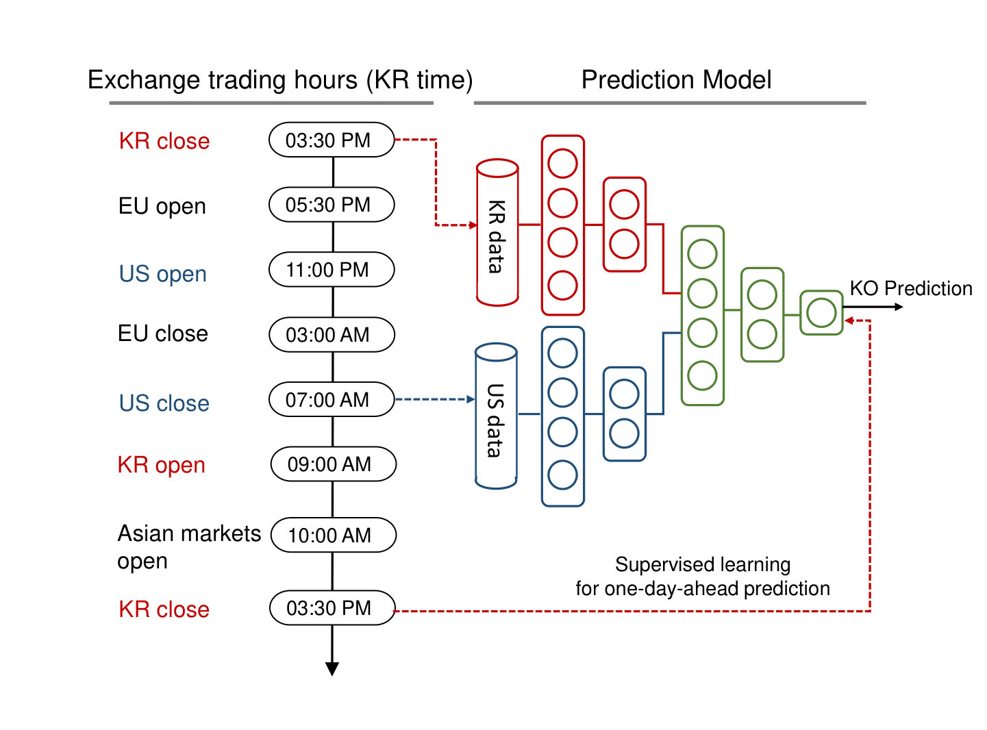 Figure 1
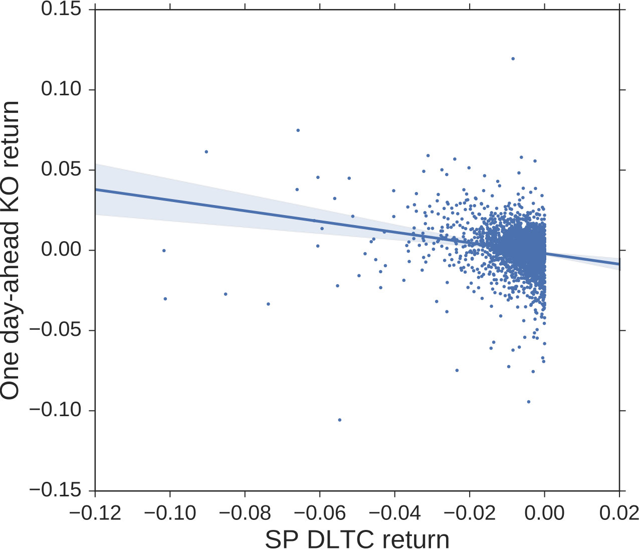 Figure 10
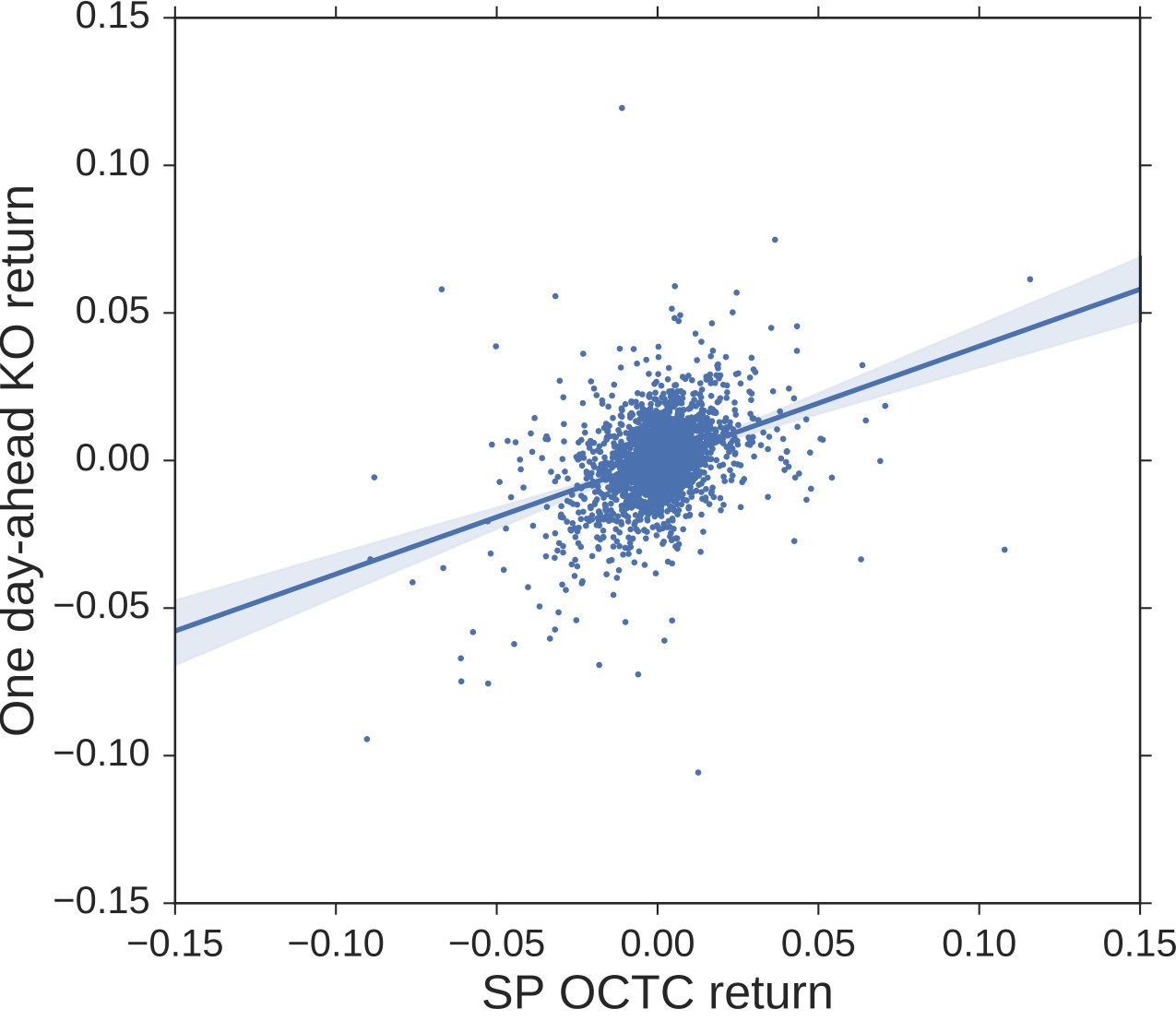 Figure 11
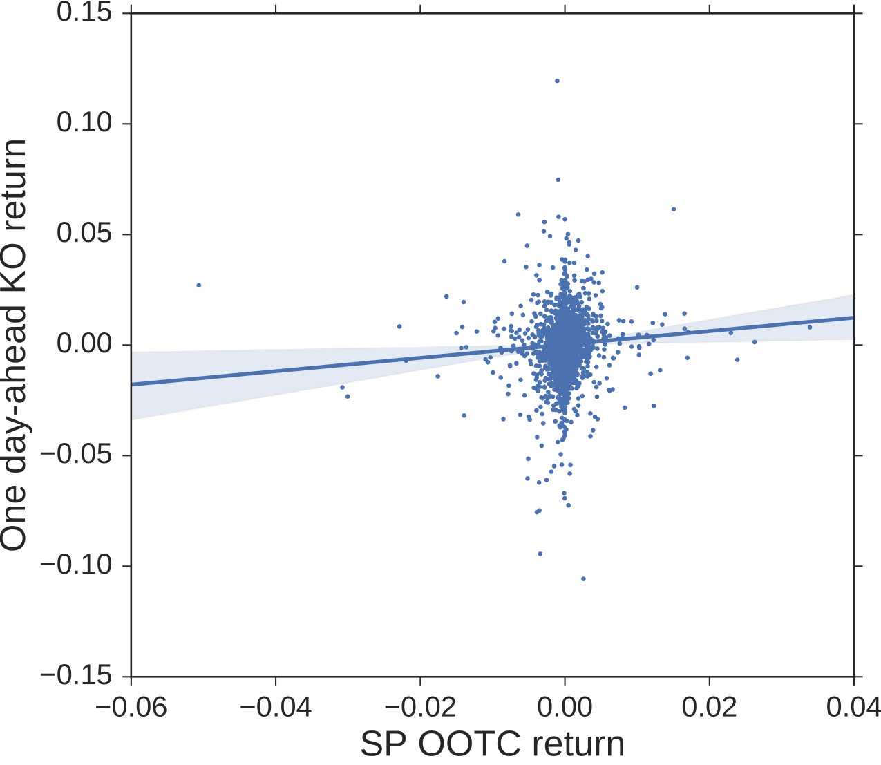 Figure 12
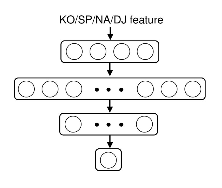 Figure 13
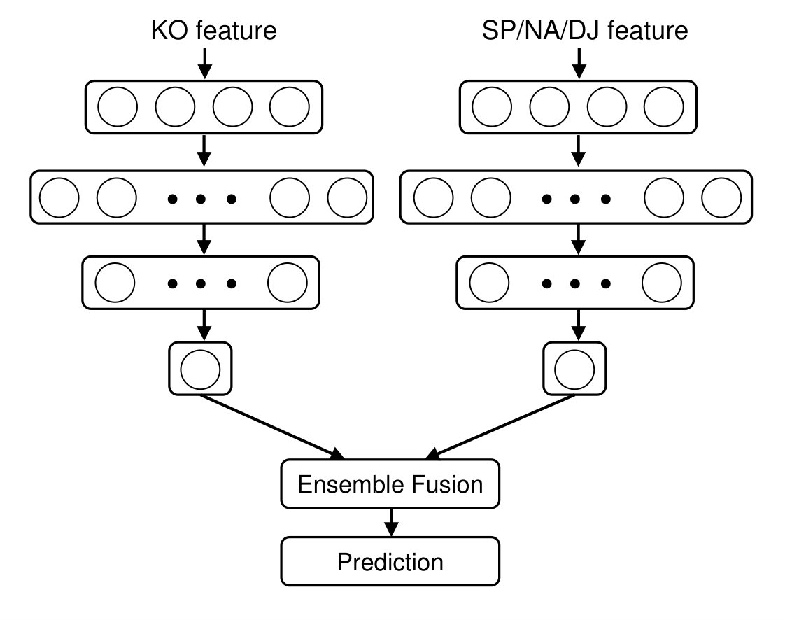 Figure 14
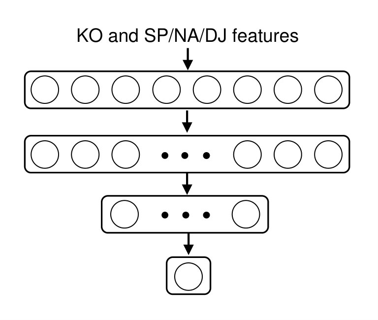 Figure 15
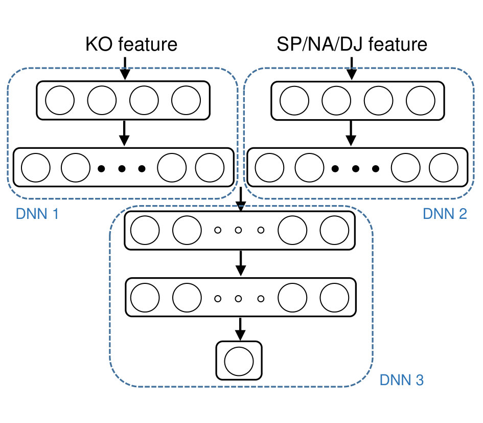 Figure 16
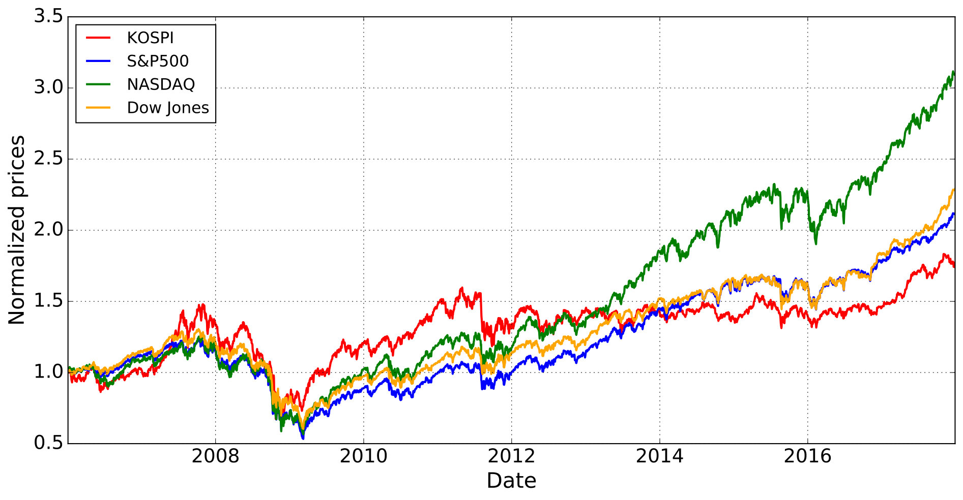 Figure 2
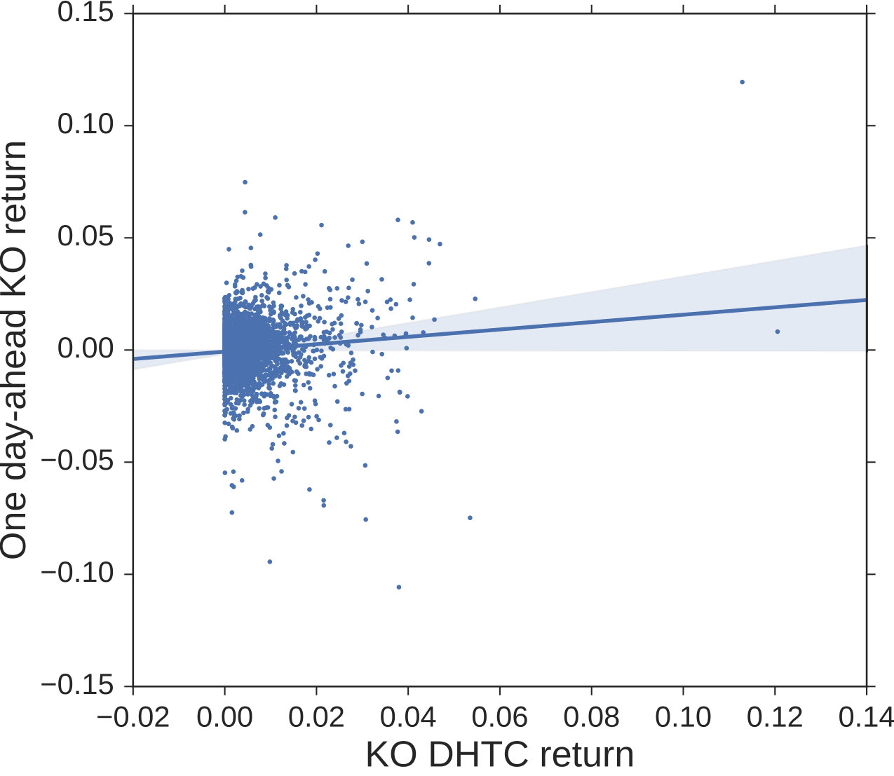 Figure 3
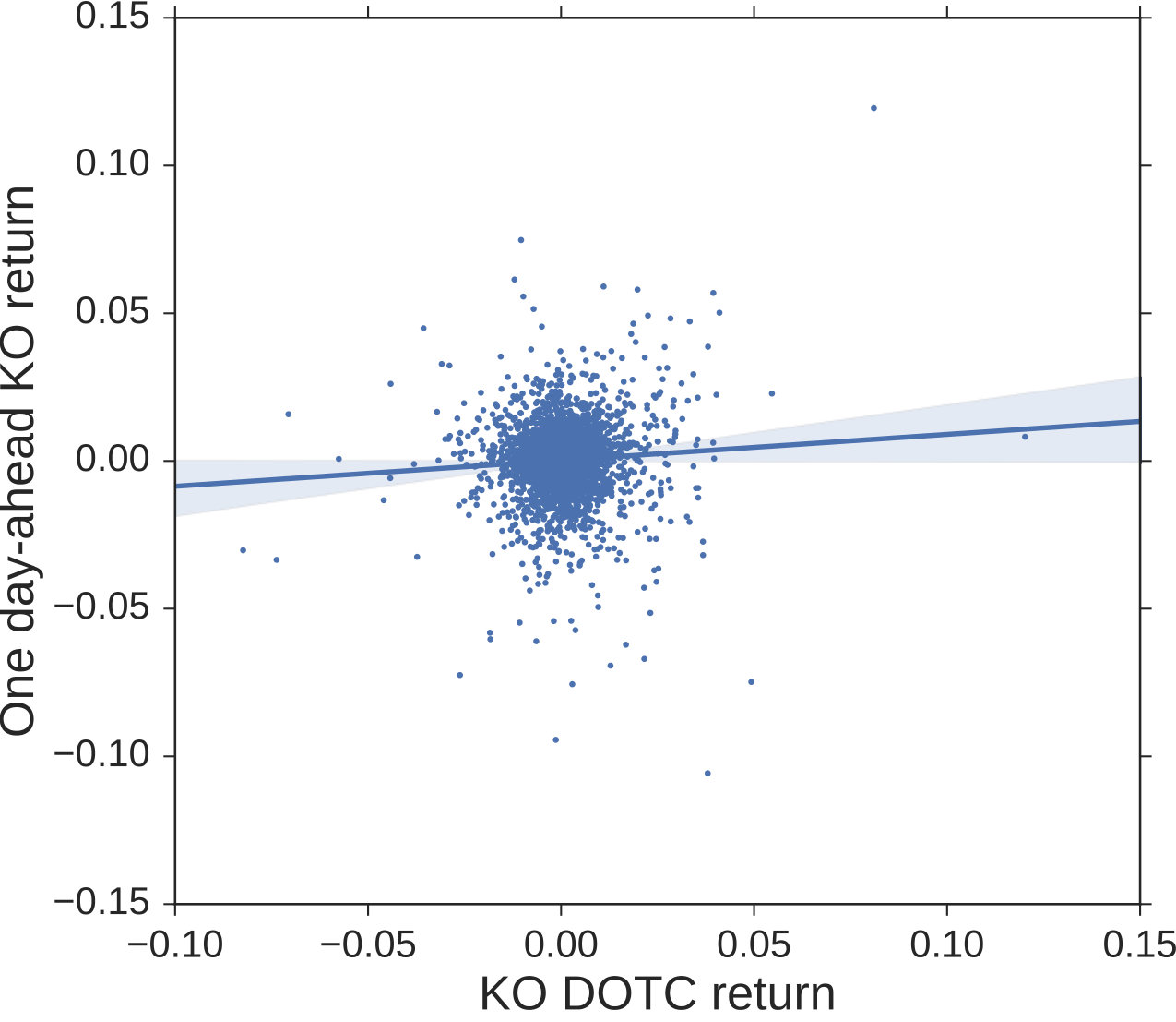 Figure 4
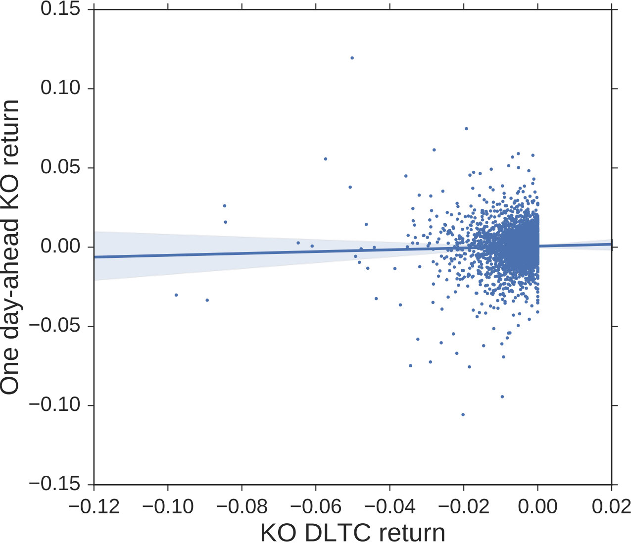 Figure 5
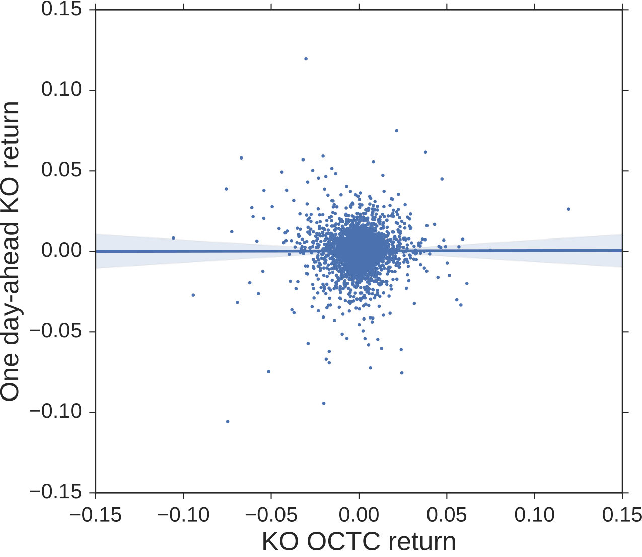 Figure 6
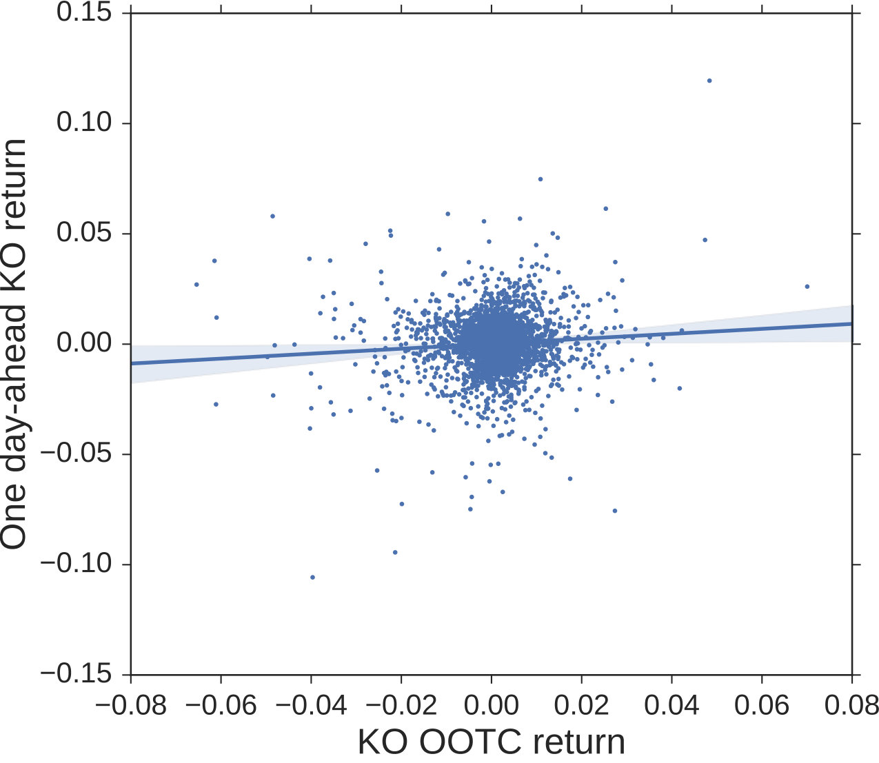 Figure 7
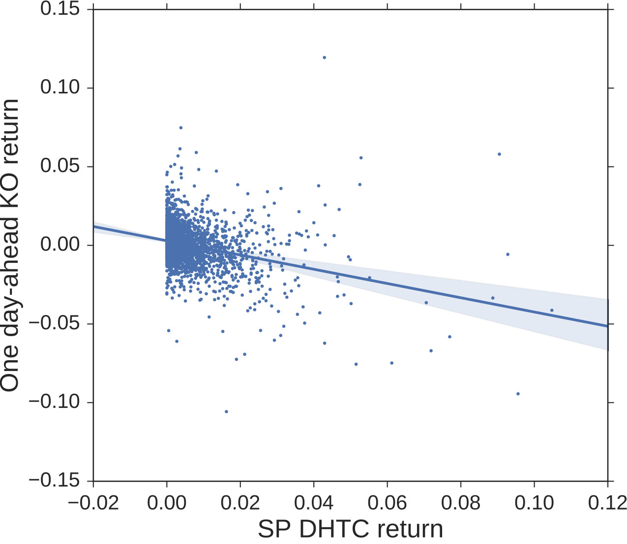 Figure 8
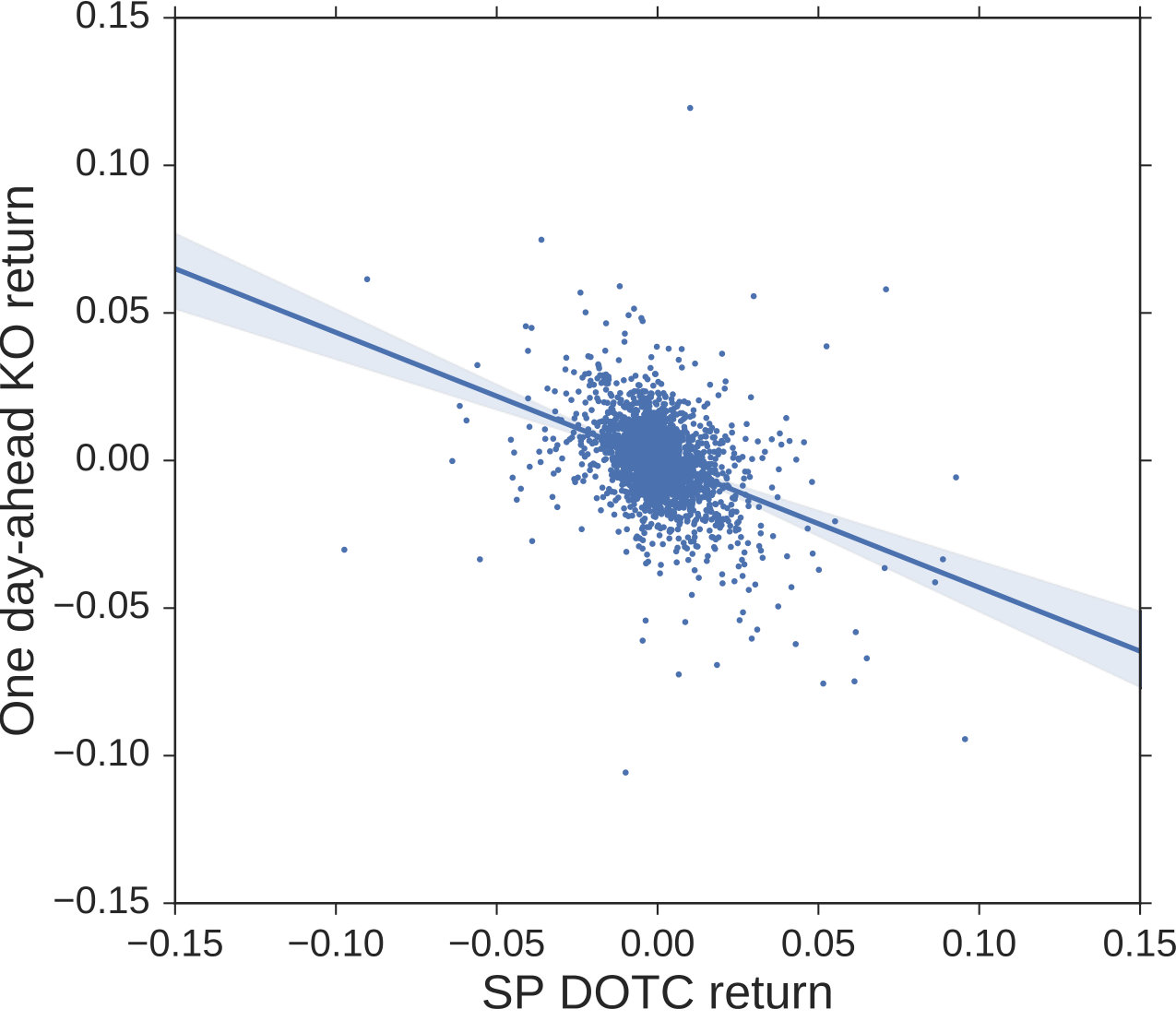 Figure 9
| Hyperparameter | Considered values/functions | |
| Number of Hidden Layers | {2, 3} | |
| Number of Hidden Units | {2, 4, 8, 16} | |
| Dropout | {0.25, 0.5, 0.75} | |
| Batch Size | {32, 64, 128} | |
| Optimizer | {RMSProp, ADAM, SGD (no momentum)} | |
| Activation Function | Hidden layer: {tanh, ReLU, sigmoid}, Output layer: Linear | |
| Learning Rate | {0.001} | |
| Number of Epochs | {100} |
| Expt. no | Momentum-based prediction-I | Momentum-based prediction-II | Buy and hold | |||
| 1 | 0.484 | 0.562 | 0.549 | |||
| 2 | 0.492 | 0.558 | 0.534 | |||
| 3 | 0.488 | 0.536 | 0.523 |
| Scaling | Non-fusion | Multimodal fusion | ||||||||
| KO-only DNN | SP-only DNN | Late | Early | Intermediate | ||||||
| Expt. 1 | ||||||||||
| 0.490 (5.257) | 0.499 (5.268) | 0.513 (5.26) | 0.609 (4.781) | 0.599 (4.989) | ||||||
| 0.526 (5.284) | 0.506 (8.787) | 0.514 (6.011) | 0.612 (4.630) | 0.592 (0.480) | ||||||
| 0.519 (5.622) | 0.500 (7.590) | 0.501 (5.851) | 0.607 (0.463) | 0.608 (4.820) | ||||||
| Expt. 2 | ||||||||||
| 0.505 (5.726) | 4.755 (6.199) | 0.479 (5.852) | 0.613 (4.951) | 0.617 (5.091) | ||||||
| 0.487 (5.717) | 4.755 (6.343) | 0.470 (5.917) | 0.615 (5.054) | 0.587 (5.193) | ||||||
| 0.484 (5.716) | 4.755 (6.437) | 0.477 (5.933) | 0.590 (4.982) | 0.648 (5.048) | ||||||
| Expt. 3 | ||||||||||
| 0.552 (3.895) | 0.549 (3.902) | 0.549 (3.891) | 0.602 (3.601) | 0.609 (3.629) | ||||||
| 0.464 (4.004) | 0.507 (4.558) | 0.500 (4.132) | 0.619 (3.680) | 0.545 (3.890) | ||||||
| 0.468 (3.991) | 0.482 (4.877) | 0.496 (4.251) | 0.584 (3.676) | 0.570 (3.700) | ||||||
| MeanSD | 0.4990.028 | 0.496 0.023 | 0.499 0.024 | 0.6060.011 | 0.5970.029 | |||||
| Scaling | Non-fusion | Multimodal fusion | ||||||||
| KO-Only DNN | NA-Only DNN | Late | Early | Intermediate | ||||||
| Expt. 1 | ||||||||||
| 0.490 (5.257) | 0.518 (5.290) | 0.500 (5.275) | 0.598 (4.774) | 0.600 (4.586) | ||||||
| 0.526 (5.284) | 0.500 (6.699) | 0.504 (5.571) | 0.594 (4.479) | 0.596 (0.478) | ||||||
| 0.519 (5.262) | 0.509 (9.565) | 0.508 (6.351) | 0.592 (0.467) | 0.605 (5.048) | ||||||
| Expt. 2 | ||||||||||
| 0.505 (5.726) | 0.484 (6.090) | 0.482 (5.823) | 0.608 (5.218) | 0.597 (5.178) | ||||||
| 0.487 (5.717) | 0.480 (6.061) | 0.486 (5.826) | 0.597 (5.071) | 0.613 (5.122) | ||||||
| 0.484 (5.716) | 0.475 (6.162) | 0.475 (5.841) | 0.580 (5.196) | 0.573 (5.221) | ||||||
| Expt. 3 | ||||||||||
| 0.552 (3.895) | 0.549 (3.908) | 0.549 (3.901) | 0.556 (3.624) | 0.605 (3.690) | ||||||
| 0.464 (4.004) | 0.471 (4.521) | 0.496 (4.962) | 0.552 (3.710) | 0.573 (3.693) | ||||||
| 0.468 (3.991) | 0.489 (4.810) | 0.489 (4.244) | 0.584 (3.648) | 0.599 (3.764) | ||||||
| MeanSD | 0.4990.028 | 0.497 0.024 | 0.4980.021 | 0.584 0.019 | 0.5950.013 | |||||
| Scaling | Non-fusion | Multimodal fusion | ||||||||
| KO-Only DNN | DJ-Only DNN | Late | Early | Intermediate | ||||||
| Expt. 1 | ||||||||||
| 0.490 (5.257) | 0.518 (5.263) | 0.515 (5.253) | 0.598 (4.774) | 0.623 (4.987) | ||||||
| 0.526 (5.284) | 0.521 (10.360) | 0.523 (7.186) | 0.607 (4.861) | 0.617 (5.539) | ||||||
| 0.519 (5.262) | 0.483 (0.701) | 0.488 (5.698) | 0.610 (0.517) | 0.609 (5.748) | ||||||
| Expt. 2 | ||||||||||
| 0.505 (5.726) | 0.473 (6.241) | 0.473 (5.861) | 0.603 (5.219) | 0.606 (5.287) | ||||||
| 0.487 (5.717) | 0.475 (6.076) | 0.482 (0.582) | 0.601 (5.161) | 0.613 (5.122) | ||||||
| 0.484 (5.716) | 0.473 (6.465) | 0.472 (5.892) | 0.592 (5.326) | 0.617 (5.694) | ||||||
| Expt. 3 | ||||||||||
| 0.552 (3.895) | 0.549 (3.906) | 0.549 (3.902) | 0.577 (3.825) | 0.580 (4.015) | ||||||
| 0.464 (4.004) | 0.482 (4.514) | 0.482 (4.093) | 0.538 (3.933) | 0.556 (3.890) | ||||||
| 0.468 (3.991) | 0.461 (4.693) | 0.482 (4.171) | 0.542 (3.878) | 0.584 (4.015) | ||||||
| MeanSD | 0.4990.028 | 0.492 0.029 | 0.4960.026 | 0.5850.027 | 0.6000.022 | |||||
Peer Reviews
No public reviews on file for this paper yet. If you reviewed it on a platform where reviews are public (OpenReview, ICLR, NeurIPS, ICML), you can paste yours below so the community can read it here.
Videos
No videos yet. Explain this paper in a talk, walkthrough, or lecture? Add one.
11institutetext: Department of Computer Engineering, Sejong University,
Seoul, Republic of Korea
{silee,sjyoo}@sejong.ac.kr
Authors’ Instructions
Multimodal Deep Learning for Finance: Integrating and Forecasting International Stock Markets
Sang Il Lee
Seong Joon Yoo
Abstract
In today’s increasingly international economy, return and volatility spillover effects across international equity markets are major macroeconomic drivers of stock dynamics. Thus, information regarding foreign markets is one of the most important factors in forecasting domestic stock prices. However, the cross-correlation between domestic and foreign markets is highly complex. Hence, it is extremely difficult to explicitly express this cross-correlation with a dynamical equation. In this study, we develop stock return prediction models that can jointly consider international markets, using multimodal deep learning. Our contributions are three-fold: (1) we visualize the transfer information between South Korea and US stock markets by using scatter plots; (2) we incorporate the information into the stock prediction models with the help of multimodal deep learning; (3) we conclusively demonstrate that the early and intermediate fusion models achieve a significant performance boost in comparison with the late fusion and single modality models. Our study indicates that jointly considering international stock markets can improve the prediction accuracy and deep neural networks are highly effective for such tasks.
Keywords:
Stock prediction, deep neural networks, multimodal, data fusion, international stock markets
1 Introduction
1.1 Aims and scope of the study
The interdependence between international stock markets has been steadily increasing in recent years. In particular, after the stock market crash of , the interdependence increased significantly [1], and more recently, this interdependence was widely noticed during the global financial crisis of [2]. Both originated in the US and resulted in a sharp decline in the stock prices of international stock markets, rapidly spreading to other countries. The crisis clearly confirmed that the financial events originating in one market are not isolated to that particular market but are also transmissible across international borders. Currently, this internationalization is a common phenomenon and expected to accelerate.
The goal of our study is to investigate the contribution of additional international market information in stock prediction by using deep learning. Typically, this interconnection has not been considered in stock prediction unlike various data categories such as country-specific price, macroeconomic, news, and fundamental data. We considered the South Korean and US stock markets with non-overlapping stock exchange trading hours as a case study and studied the one-day ahead stock return prediction of the South Korean stock market by combining the data of the two markets. The combination of the markets is particularly fascinating due to their different behaviors: the US markets have a long-run upward trend whereas the South Korean markets do not. Therefore, the possible existing correlations between them are not just the result of the continued global economic growth. We utilized the daily trading data (i.e., opening, high, low, and closing prices) of both markets, which is publicly available and quantifies the daily movement of the markets. The publicity ensures that our results are more likely to be independent and easily integrated with other data, serving as a prototypical model.
We designed multimodal deep learning models to extract cross-market correlations by concatenating features at early, intermediate, and late fusions between modalities. The models places a different emphasis on intra and inter market correlations depending on the markets to be tested. The experiments showed that the early and intermediate fusions achieve better prediction accuracy than the single modal prediction and late fusions. This indicates that multimodal deep learning can capture cross-correlations from stock prices despite their low signal-to-noise ratio. It also indicates that, when optimizing prediction models, cross-market learning provides opportunities to improve the accuracy of stock prediction, even when the shared trends in markets are scarce.
The remainder of this paper is organized as follows. Section 1.2 discusses the connections to existing work. Section 2 introduces the US and South Korean (KR) international stock markets. Section 3 discusses data and preprocessing methods. Section 4 describes a basic architecture for deep neural networks and illustrates three prediction models. Section 5 presents information on the training of the deep neural networks. Section 6 presents the prediction accuracy of the models and discusses their capacity. Finally, Section 7 presents the concluding remarks and future scope of the study.
1.2 Connections with previous studies
Over the past few decades, machine learning techniques, such as artificial neural networks (ANNs), genetic algorithms (GAs), support vector machines (SVM), and natural language processing (NLP), have been widely employed to model financial data. For example, a genetic classifier designed to control the activation of ANNs [3], the genetic algorithms approach to feature discretization in ANNs [4], the wavelet de-noising-based ANN [5], wavelet-based ANN [6], and the surveys on sentiment analysis [7] and machine learning [8, 9].
Machine learning techniques help to mitigate the difficulties in modeling, such as the existence of nonlinear behaviors in financial variables, the non-stationarity of relationships among the relevant variables, and a low signal-to-noise ratio. In particular, deep learning is becoming a promising technique for modeling financial complexity, owing to its ability to extract relevant information in complex, real-world world data [10]. For example, stock prediction based on long short-term memory (LSTM) networks [11], deep portfolios based on deep autoencoders [12], threshold-based by using recurrent neural networks [13], and deep factor models involving deep feed-forward networks [14], and LSTM networks [15].
A major challenge for further research in this area is the simultaneous consideration of the numerous factors in financial data modeling. In the search for factors that explain the cross-sectional expected stock returns, numerous potential candidates have been found by using econometric models. For example, accounting data, macroeconomic data, and news [16, 17, 18, 19, 20]. Stock price predictions that consider a few pre-specified factors may lead to incorrect forecasting as they reflect partial information or an inefficient combination of the factors. Thus, currently, one of the most important tasks in finance is to develop a method that effectively integrates diverse factors in prediction processes.
A few recent studies have begun to combine financial data using deep learning. Xing et al. [21] dealt with the price, volume, and sentiment data to build a portfolio using LSTM networks. Bao et al. [22] used trading data (prices and volume), technical indicators, and macroeconomic data (exchange and interest rates) to predict stock prices by combining the wavelet transforms (WT), stacked autoencoders (SAEs), and LSTMs. The fusion strategy of these studies concatenates the data into the input layers, known as an early fusion. However, because hidden layers in such approaches are exposed to cross-modality information, it could be more difficult to use them specifically to extract the essential intra-modality relations during training. In this study, to effectively integrate financial data, we introduce a systematic fusion approach, i.e., early, intermediate, and late fusions, by considering the international stock markets as a case study.
International market dynamics has been a controversial issue in financial academia and industries due to the increasing economic globalization. Although stock market integration is intuitively obvious in an era of free trade and globalization, the underlying mechanisms are highly complex and not easily understood. Financial economists have developed models for describing The dynamic interdependency among major world stock exchanges using econometric tools such as vector autoregression (VAR) and autoregressive conditional heteroskedastic (ARCH) models [23, 24]. They have attempted to find underlying reasons behind the interdependence, providing possible scenarios of mechanisms in terms of deregulation [25, 26], international business cycles [27], regional affiliations and trade linkages [28], and regional economic integration [29]. However, despite the advantage of such approaches in explaining the underlying mechanism, they generally only deal with a small number of financial variables; and as a result describe only a partial aspect of the complex financial reality, which is actually characterized by multidimensional and nonlinear characteristics. Thus, international markets are a good case study for the effectiveness of deep learning in financial data fusion. Furthermore, modeling international markets is important in practice because investors and portfolio managers need to continually assess international information and adjust their portfolios accordingly, in order to take the benefits of portfolio diversification [30].
Technically, we were inspired by the success of the multimodal deep learning technique [31, 32, 33] in computer science. The main advantage of deep learning is the ability to automatically learn hierarchical representations from raw data, which can then be extended to cross-modality shared representations at different levels of abstraction [31, 33]. Multimodal deep learning has been widely applied to multiple channels of communication, such as auditory (words, prosody, dialogue acts, and rhetorical structure) and visual (gesture, posture, and graphics), achieving better prediction accuracy than approaches using only single-modality data.
2 International stock markets: US and KR
We consider two international stock markets of South Korea (KR) and the US. They are effective cases for studying the spillover effect because the trading time horizons of these markets do not overlap. The US stock market opens at 9:30 a.m. and closes at 4:00 p.m. (EST time), whereas the KR stock exchange opens at 9:00 a.m. and closes at 3:30 p.m. (KST time). The KR market opens three hours after the US market closes. Due to the non-overlapping time zones, the closing prices of the US market index affect the opening prices of the KR market index, and vice versa.
There is significant empirical evidence on the correlative behavior between the two markets. Na and Sohn [34] investigated the co-movement between the Korea composite stock index (KOSPI) and the world stock market indexes using association rules. They found that the KOSPI tends to move in the same direction as the stock market indices in the US and Europe, and in the opposite direction to those in other East Asian counties, including both Hong Kong and Japan, which have competitive relationships with KR. Jeon and Jang [35] found that the US market plays a leading role in the KR stock market by applying the vector autoregression (VAR) model to the daily stock prices in both nations. Lee [36] statistically showed a significant volatility spillover effect between them.
Overall, the results of previous studies based on traditional financial models and primarily linear regression models, have consistently demonstrated the existence of an interrelationship between the two markets by identifying statistically significant explanatory variables. The objective of this study is to capture this interrelationship by using multimodal deep learning and utilize it as complementary information for stock prediction. Figure 1 shows a schematic diagram of the model that integrates the KR and US stock market prices and predicts the KR market (the neural network will be discussed in detail in Section 4).
3 Data and preprocessing
3.1 International Market Indexes
We used the KOSPI (KO) index as a proxy of the KR stock markets and the Standard and Poor’s 500 (SP), NASDAQ (NA), and Dow Jones Industrial Average (DJ) indexes as proxies of the US stock market. The KO is a highly representative index of the KR stock markets as it tracks the performance of all common shares listed on the KR stock exchange, based on capitalization-weighted schemes. The DJ is a price-weighted index composed of 30 large industrial stocks. The SP is a value-weighted index of 500 leading companies in diverse industries of the US economy. The SP index covers 80 of the value of US equities and therefore provides an aggregate view of overnight information in the United States. The NA is weighted by capitalization of the stocks included in its index and contains stocks in large technology firms, such as Cisco, Microsoft, and Intel.
3.2 Raw data
The daily market data for the four indexes are obtained from Yahoo Finance and contain daily trading data, such as opening prices (Open), high prices (High), low prices (Low), adjusted closing prices (Close), and end-of-day volumes. The data are from the period between January 1st, 2006 and December 31st, 2017 (Fig. 2). The data from days where either one of the stock markets was closed was excluded from our data set.
3.3 Training, validation, and test set
All data are divided into a training dataset (70) for developing the prediction models and test set (30) for evaluating its predictive ability. 30 of the training set was used as a validation set.
3.4 Feature construction
We seek predictors in order to predict the daily (close-to-close) KO return at time , given the feature vector extracted from the trading data available at time . To describe the movement of the indexes, we defined a set of meaningful features at time as follows:
, 2. 2.
, 3. 3.
, 4. 4.
, 5. 5.
.
The features describe the daily movement of stock indexes: for the highest daytime movement, for the lowest daytime movement, for the daytime movement, for the opening jump responding to the overnight information, and for the total movement reflecting all information available at time .
Let us denote the feature vector for each modality as , where , and . An input feature for multimodal models at time is the combination of and , depending on the multimodal deep learning architecture. Note that we did not include returns across markets, such as SP Close-to-KO Close return=, because they are statistically non-stationary at any conventional significance level. In the following, we will use the notation and interchangeably to denote the daily close-to-close return on the KO index.
To improve the accuracy of the prediction and prevent complications arising from convergence during training, we normalized the individual feature into the range , using the following formula:
[TABLE]
where on the right side represents the normalized value of data on the right side; and denote the maximum and minimum values of data , respectively; these were estimated using only the training set to avoid look-ahead biases and then applied to the validation and test sets.
3.5 Association of the two markets
For an intuitive understanding, we visualize the patterns between the features and target by using scatter plots with a regression best-fit line. Figure 3 shows the scatter plots for the pairs of KO features and the one-day-ahead returns. There is an extremely weak positive linear association, which is described by the shallow slopes of the regression lines from 0.002 to 0.164 and significant variation around the linear regression lines. As shown in Fig. 4, the scatter plots for the SP features exhibit more diverse patterns, i.e., positive as well as negative slopes, with relatively steeper slopes from to 0.385 and significant variation around the linear regression lines. The steeper slopes exhibit a certain extent of a spillover effect from the US daytime stock market to the next day KR stock market. This implies that the US and KR markets share a certain amount of information. We ultimately intend to capture this information by using multimodal deep learning.
4 Multimodal deep learning network model
4.1 Deep neural network
The multimodal deep neural network consists of deep neural networks (DNNs), which are a sequence of fully connected layers. The DNN can extract high-level features from raw data through statistical learning over a large amount of data to obtain an effective representation of input data.
Suppose that we are given a training data set and a corresponding label set , where denotes the number of days in the period of the training set. The DNN consists of an input layer , an output layer , and H hidden layers between the input and output layers. Each hidden layer is a set of several units, which could be arranged as a vector , where denotes the number of units in . The units in are recursively defined as a nonlinear transformation of the -th layer:
[TABLE]
where the weight matrix , the bias vector , and , where the weight matrix . The nonlinear activation function acts entry-wise on its argument and the units in the input layer are the feature vectors. According to the daily return regression task, a single unit with a linear activation function in the output layer is used in the output layer . Then, given the input , the one day-ahead return prediction is given by
[TABLE]
where and is the unit in the final hidden layer .
4.2 Single and multimodal deep networks for stock prediction
We built the prediction models based on early, intermediate, and late fusion frameworks.
Single modal models (baseline): To compare the performance of the fusion models, we used four types of single modal models: (1) KO-Only DNN, (2) SP-Only DNN, (3) NA-Only DNN, and (4) DJ-Only DNN models (left-hand side of Fig. 5). Their training sets are given by , , , and , respectively.
Early fusion: The input feature vectors are simply concatenated together at the input layer and then processed together throughout the DNN (left-hand side of Fig. 6). The feature vector is given by
[TABLE]
where we use to denote the concatenation of the two vectors and . Although this model is computationally efficient as compared to the other fusion models, as it requires a lower number of parameters, it has several drawbacks [37] such as over-fitting in the case of a small-size training sample and the disregard of the specific statistical properties of each modality.
Intermediate fusion Intermediate fusion combines the high-level features learned by separate network branches (right-hand side of Fig. 6). The network consists of two parts. The first part consists of three independent deep neural networks, i.e., DNN1, which extracts features from the input feature , DNN2, which extracts features from the input feature , and DNN3, which fuses the extracted features and forecasts returns. The input feature vector of DNN3 is given by
[TABLE]
where and are the units of DNN1 and DNN2, respectively. These fusions are not exposed to cross-modality information at the raw data level and consequently, reveal more intra-modality relationships than the early fusion model.
Late Fusion Late fusion refers to the aggregation of decisions from multiple predictors (right-hand side of Fig. 5). Let and be the predictions from the individual DNNs. Then, the final prediction is
[TABLE]
where is a rule combining the individual predictions, such as averaging [38], voting [39], or learned model [40, 41], to generate the final results. In this study, we used the linear rule given by
[TABLE]
is a weight to combine the prediction values from the KO and US data. Here, is a mixing parameter that determines the relative contribution of each modality to the combined semantic space. We set , so that the KO and US sources contribute equally to the final prediction results.
All neural networks are trained by minimizing the mean squared error (MSE), , on the validation set.
Financial implications of fusion at different levels
It would be financially meaningful to distinguish between fusion levels when international financial markets are combined. The price of domestic stock is commonly influenced by foreign events, but the degree of that influence depends on the international financial interdependency of the domestic stock market. Developed financial markets are likely to be highly exposed to international events and exhibiting high international correlations. In contrast, underdeveloped markets are likely to be isolated and exhibiting low international and high intra-national correlations. Early fusion would be more suitable for developed markets in the sense that it can directly capture cross-correlations between domestic and foreign features in a single concatenation layer. In contrast, the intermediate fusion would be more suitable for underdeveloped (or developing) markets in the sense that domestic features are more likely correlated with each other than with external foreign markets.
5 Training
To find the best configuration, we used the tree-structured Parzen estimators (TPE) algorithm [42] , as one of the Bayesian hyper-parameter optimizations, which is capable of optimizing more hyperparameters simultaneously (Table 1). The hyper-parameters include: the number of layers, the number of hidden units per layer, the activation function for a layer, the batch size, the optimizer, the learning rate, and the number of epochs. We apply the back-propagation algorithm [45, 46] to get the gradient of our models, without any pre-training, meaning that deep networks can be trained efficiently with ReLU without pre-training [47]). All network weights were initialized using Glorot normal initialization [48].
5.1 Regularizations
We used three types of regularization methods to control the overfitting of the networks and to improve the generalization error, including dropout, early stopping, and batch normalization.
Dropout. The basic idea behind dropout is to temporarily remove a certain portion of hidden units from the network during training time, with the dropped units being randomly chosen at each and every iteration [49]. This reduces the co-adaptation of the units, approximates model averaging, and provides a way to combine many different neural networks. In practice, dropout regularization requires specifying the dropout rates, which are the probabilities of dropping a neuron. In this study, we inserted dropout layers after every hidden layer, and performed a grid-search over the dropout rates of 0.25, 0.5, and 0.75 to find an optimal dropout rate for every architecture (Table 1).
Batch Normalization The basic idea of batch normalization (BN) is similar to that of data normalization in training data pre-processing [50]. The BN technique uses the distribution of the summed input to a neuron over a mini batch of training cases to compute the mean and variance, which are then used to normalize the summed input of that neuron on each training case. There is a lot of evidence that the application of batch normalization results in even faster convergence of training, increasing the accuracy compared to the same network without batch normalization [50].
Early Stopping. Another approach we used to prevent overfitting is early stopping. Early stopping involves freezing the weights of neural networks at the epoch, where the validation error is minimal. The DNNs, which were trained with iterative back propagation, were able to learn the specific patterns of the training set after every epoch, instead of the general patterns, and begun to over-fit at a certain point. To avoid this problem, the DNNs were trained only with the training set, and the training was stopped if the validation MSE ceased to decrease for 10 epochs.
6 Experiments
6.1 Evaluation metric
It is often observed that the performance of stock prediction models depends on the window size used. To make the evaluation task more robust, we conducted experiments over three different windows: (1) Expt. 1 from 01-Jan-2006 to 31-Dec-2017; Expt. 2 from 01-Jan-2010 to 31-Dec-2017; and Expt. 3 from 01-Jan-2014 to 31-Dec-2017.
After obtaining the predictions for the test data, they were denormalized using the inverse formula of Eq. (1). Hereafter, denotes the denormalized prediction. Given a test set and a corresponding level , where denotes the number of days in the test sample. We evaluate the prediction performance using the MSE and the hit ratio defined as follows:
[TABLE]
where is the directional movement of the prediction on the trading day, defined as:
[TABLE]
6.2 Daily strategies as baselines
To evaluate the single and fusion models, we examined the hit ratios for the three regular rules:
- •
Momentum-based prediction-I: If the KOSPI index rises (falls) today, it predicts that the KOSPI index will rise (fall) tomorrow too.
- •
Momentum-based prediction-II: If the SP500 index rises (falls) today, it predicts that the KOSPI index will rise (fall) tomorrow too.
- •
Buy and holding strategy: Based on positive historical returns, it predicts that the KOSPI index of the next day will rise.
Table 2 shows that the momentum-based prediction-II is the most accurate of the three rules, exhibiting hit ratios of 0.562, 0.558, and 0.536 for Expt. 1, Expt. 2, and Expt. 3, respectively.
6.3 Results
We present the prediction results obtained with the fusion models for the pairs of KO and SP features (Table. 3), the KO and NA features (Table 4), and the KO and DJ features (Table 5), along with those of non-fusion models for each of the country-specific features as a baseline model. To remove potentially undesirable variances that arise from parameters having different min-max ranges, we also conducted the experiments with three distinct ranges , , and . The main findings are follows:
Early vs. intermediate fusion For the fusion of the KO and SP features (Table 3), the mean hit ratio (directional prediction) of the early fusion () is slightly higher or comparable to that of the intermediate fusion (). For the fusion of the KO and NA features (Table 4), the hit ratio of early fusion () is slightly lower or comparable to that of the intermediate fusion (). For the fusion of the KO and DJ features (Table 5), the hit ratio of the early fusion () is slightly lower or comparable to that of the intermediate fusion (). Thus, the performance of the two fusion approaches are comparable overall, which is consistent over the different window sizes and the min-max ranges. In terms of computational efficiency, the early fusion model is more attractive due to its lower number of parameters compared to the intermediate fusion model.
Single vs. multimodality The overall hit ratio of the single modal models is about 0.49: 0.4990.028 for the KO-Only DNN, 0.4960.023 for the SP-Only DNN (Table 3), 0.4970.024 for the NA-Only DNN (Table 4), and 0.4920.029 for the DJ-only DNN (Table 5). Interestingly, the performances are slightly worse than the momentum-based prediction-II (approximately 0.55) and the buy and hold strategy (approximately 0.53). The hit ratios of the late fusion are for the KO and SP fusion, for the KO and NA fusion, and for the KO and DJ fusion, which are lower than those of the early and intermediate fusions. These results show that the parameters of the two modalities needs to be estimated jointly. The poor performance of the single modality models clearly emphasizes the importance of multimodal integration to leverage the complementarity of stock data and provide more robust predictions.
7 Discussion and conclusion
We developed stock prediction models that combine information from the South Korean and US stock markets by using multimodal deep learning. We exploited DNN as a branch of deep learning to take advantage of its strong capability in non-linear modeling and designed three types of architectures to capture the cross-modal correlation at different levels. Experimental results show that the early and intermediate fusion models predict stock returns more accurately than the single modal and late fusion models, which do not consider cross-modal correlation in their predictions. This indicates that joint optimization can effectively capture complementary information between the markets and assist in the improvement of stock predictions.
This study has a few limitations. First, we examined three different time periods of , , and . Over these periods, the early and intermediate fusion model consistently outperformed the regular rule-based prediction and late fusion models, in terms of accuracy. However, the sample sizes of the present study are relatively small, and the performance of the models may vary based on the period and depending on the globalization level of the stock markets. Second, the information of international markets is limited to trading data.
Future works will focus on two aspects. First, we plan to include more diverse information sources such as fundamental data and sentiment indexes. The stock prices are determined by the supply and demand of the stocks, which occurs due to various information inputs. Thus, integrating more diverse data would lead to an improvement in the reliability of stock prediction. Second, we plan to analyze the prediction results by using explainable machine learning techniques. Understanding and interpreting prediction models are crucial in financial fields.
Acknowledgments
This work was supported by the ICT RD program of MSIP/IITP [2017-0-00302, Development of Self Evolutionary AI Investing Technology].
The reference list from the paper itself. Each links out to its DOI / PubMed record.
- 1[1] Eun, C. and Shim, S. International transmission of stock market movements. Journal of Financial and Quantitative Analysis. 24, 241–256 (1989).
- 2[2] Bekaert, G., Hodrick, R. J., and Zhang, X. International stock return comovements. The Journal of Finance. 64, 2591–626 (2009).
- 3[3] Armano, G., Marchesi, M., and Murru, A. A hybrid genetic-neural architecture for stock indexes forecasting. Information Sciences, 170, 3–33 (2005).
- 4[4] Kim, K. and Han, I. Genetic algorithms approach to feature discretization in artificial neural networks for the prediction of stock price index. Expert Systems with Applications. 19, 125–132 (2000).
- 5[5] Wang, J.-Z., Wang, J.-J., Zhang, Z.-G., and Guo, S.-P. Forecasting stock indices with back propagation neural network. Expert Systems with Applications. 38 (11), 14346–14355 (2011).
- 6[6] Saadaoui, F. and Rabbouch, H. A wavelet-based multiscale vector-ANN model to predict comovement of econophysical systems. Expert Systems with Applications. 41 (13), 6017–6028 (2014).
- 7[7] Frank Z. X., Cambria, E., and Welsch, R. E. Natural language based financial forecasting: a survey. Artif Intell Rev. 50, 49–73 (2018).
- 8[8] Atsalakis, G. S. and Valavanis, K. P. Surveying stock market forecasting techniques–part ii: soft computing methods. Expert Systems with Applications. 36 (3), 5932–5941 (2009).