Laws of large numbers for the frog model on the complete graph
Elcio Lebensztayn, Mario Andres Estrada

TL;DR
This paper investigates the frog model on complete graphs, proving that as the number of vertices grows large, the process's behavior can be approximated by a deterministic dynamical system, revealing insights into epidemic spreading dynamics.
Contribution
The paper establishes laws of large numbers for the frog model on complete graphs, connecting stochastic processes to deterministic dynamical systems for large network sizes.
Findings
Process approximated by 3D dynamical system as N→∞
Long-term behavior of the deterministic system analyzed
Different lifetime models for active particles studied
Abstract
The frog model is a stochastic model for the spreading of an epidemic on a graph, in which a dormant particle starts to perform a simple random walk on the graph and to awake other particles, once it becomes active. We study two versions of the frog model on the complete graph with vertices. In the first version we consider, active particles have geometrically distributed lifetimes. In the second version, the displacement of each awakened particle lasts until it hits a vertex already visited by the process. For each model, we prove that as , the trajectory of the process is well approximated by a three-dimensional discrete-time dynamical system. We also study the long-term behavior of the corresponding deterministic systems.
Click any figure to enlarge with its caption.
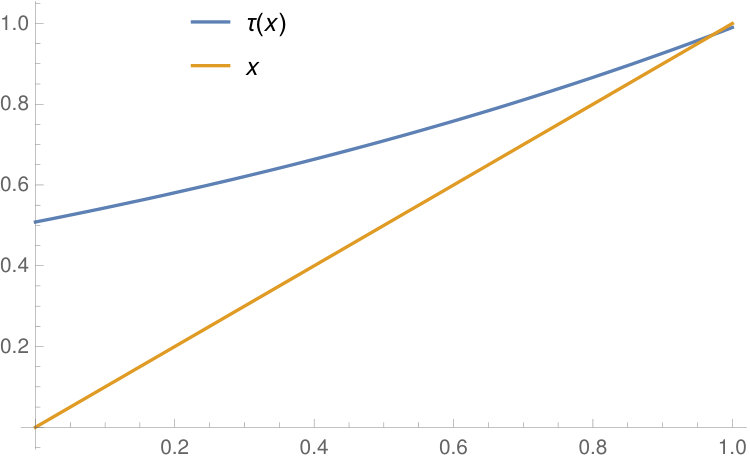 Figure 1
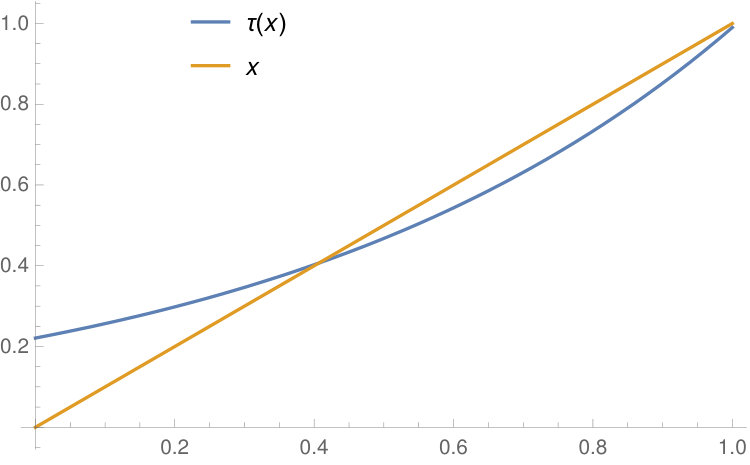 Figure 2
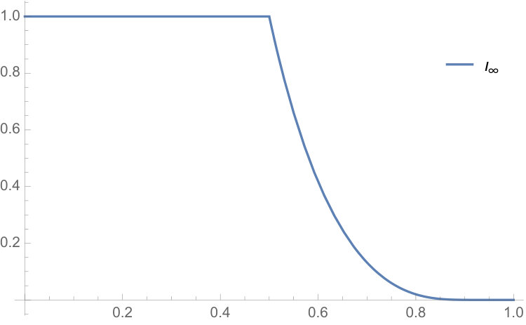 Figure 3
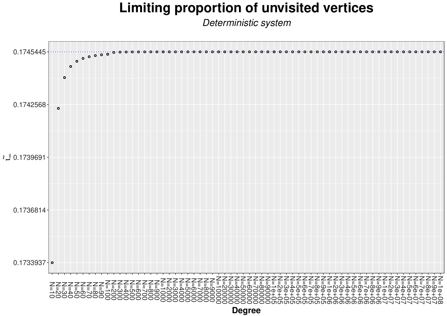 Figure 4
Peer Reviews
No public reviews on file for this paper yet. If you reviewed it on a platform where reviews are public (OpenReview, ICLR, NeurIPS, ICML), you can paste yours below so the community can read it here.
Videos
No videos yet. Explain this paper in a talk, walkthrough, or lecture? Add one.
Laws of large numbers for the frog model
on the complete graph
Elcio Lebensztayn
Institute of Mathematics, Statistics and Scientific Computation
University of Campinas – UNICAMP
Rua Sérgio Buarque de Holanda 651, 13083-859, Campinas, SP, Brazil.
and
Mario Andrés Estrada
Abstract.
The frog model is a stochastic model for the spreading of an epidemic on a graph, in which a dormant particle starts to perform a simple random walk on the graph and to awake other particles, once it becomes active. We study two versions of the frog model on the complete graph with vertices. In the first version we consider, active particles have geometrically distributed lifetimes. In the second version, the displacement of each awakened particle lasts until it hits a vertex already visited by the process. For each model, we prove that as , the trajectory of the process is well approximated by a three-dimensional discrete-time dynamical system. We also study the long-term behavior of the corresponding deterministic systems.
Key words and phrases:
Frog model, Law of large numbers, random walks, complete graph.
2010 Mathematics Subject Classification:
60K35, 60J10, 92B05
Elcio Lebensztayn is thankful to the National Council for Scientific and Technological Development – CNPq, and Mario Andrés Estrada is thankful to the Coordination for the Improvement of Higher Education Personnel – CAPES, for financial support. Both authors are also grateful to the São Paulo Research Foundation – FAPESP (grant 2017/10555-0).
1. Introduction
We study stochastic systems whose agents are particles with random lifetimes, that move along the vertices of a finite graph. These systems, referred to as frog models, are commonly idealized with the motivation of modeling the spreading of a rumor or epidemic through a population. Our main purpose is to prove limit theorems that allow us to identify the deterministic system (in discrete time) that approximates the trajectory of the process, when the graph size becomes large.
To define the models under study, for , let denote the complete graph with vertices. At time zero, there is one particle at each vertex of , all of them are sleeping, except for that placed at a fixed vertex of the graph. Once wakened, particles perform independent simple random walks on in discrete time. When a vertex with a sleeping particle is visited for the first time, that particle is activated and starts its own random walk. However, each active particle has a random lifetime. In the first model we consider, before each jump, active particles choose either to survive with probability or to disappear with probability , independently of each other. That is, upon being activated, a particle dies after a random number of jumps, having geometric distribution with parameter . We call this process the geometric model. In the second model we study, which we refer to as the nongeometric model, each active particle survives up to the time it hits a vertex which has been visited before by the process. In epidemic terms, the active particles are pathogenic agents, which move along the vertices of the graph (individuals). Whenever a virus jumps onto a susceptible individual (an unvisited vertex), this individual becomes infected, and the virus duplicates. In the geometric model, viruses have independent trajectories and lifetimes. In the nongeometric model, once visited, a vertex activates an antivirus which kills every virus that tries to infect it in the future. We study the fundamental question concerning how the proportion of visited vertices (infected individuals) evolves throughout the process.
Both systems of random walks on the complete graph are analyzed in Alves et al. [3]. For the geometric model, the authors prove that a critical parameter related to the final epidemic size equals . For the nongeometric model, the results are derived from computational analysis, simulations and mean field approximation. In our work, motivated by the results and open questions presented there, we establish a law of large numbers which guarantees that the sample paths of the stochastic process stay close to the solution of a discrete dynamical system. For the geometric model, the corresponding deterministic system is a discrete-time version of the classical epidemic model proposed by Kermack and McKendrick [24, 25], whereas for the nongeometric model it is the dynamical system found by Alves et al. [3] through a mean field approximation approach. In addition, for both models, we study the long-term behavior of the associated deterministic systems. The results are stated in Section 2.
We point out that limit theorems of the type we derive are well-known for continuous-time Markovian processes; see Barbour [4], Ethier and Kurtz [13, Chapter 11] and Darling and Norris [12]. Regarding the frog model, Kurtz et al. [26] and Lebensztayn [27] obtain limit theorems for the final outcome of different types of the continuous-time system on the complete graph. Machado et al. [34] deal with a discrete-time model also on the complete graph, in which a unique active particle is allowed to jump at each instant of time. Differently from these three papers, in our models, several particles can jump simultaneously, so that the transitions may be abrupt. With respect to other processes in discrete time, Buckley and Pollett [7] prove limit theorems for a class of one-dimensional chain binomial models, and other models with similar characteristics. As we will see in the sequel, the systems that we study are described by Markov chains taking values in , whose general structures do not fulfill the conditions of the theorems stated in that paper (since the functions that one uses to describe our density processes depend upon and ; see, in particular, Lemmas 3.1, 3.2, 3.5 and 3.6). The techniques we develop here are inspired by the methods presented in Buckley and Pollett [7].
A brief overview on the frog model
Besides the epidemic perspective, modeling combustion chemical reactions provides another interpretation for the frog model. In this case, the systems are often formulated in continuous time; see, e.g., Comets et al. [9], Ramírez and Sidoravicius [38], and Rolla and Sidoravicius [39].
The model has been primarily studied on infinite graphs, such as the integer lattices , homogeneous trees and -ary trees. In the case when the frogs have geometrically distributed lifetimes, there exists a critical value of the parameter below which the system dies out almost surely. This critical phenomenon is an important topic of research; see Alves et al. [1], Fontes et al. [14], Lebensztayn and Utria [30, 31], and references therein. The issue of survival is also addressed for similar models on in Bertacchi et al. [6] and Lebensztayn et al. [33].
When active frogs live forever, other fundamental questions are considered, such as: (i) whether the root vertex of the graph is visited by frogs infinitely often; and (ii) how the set of visited vertices grow and the cloud of particles move. With respect to (i), Telcs and Wormald [42] establish that the frog model starting with one particle per vertex is recurrent on , for every . A threshold result on , with Bernoulli initial configuration, is derived by Popov [36]. Recurrence and transience on infinite trees was a prominent open question until recently. Hoffman et al. [18] establish that the frog model is recurrent on the binary tree, but it is transient on -ary trees, for . We also refer to Hoffman et al. [17], Johnson and Junge [23] and Rosenberg [40]. The subjects in (ii) are investigated mainly for processes on (see, for instance, Alves et al. [2], Ramírez and Sidoravicius [38], Höfelsauer and Weidner [16]), and lately analyzed on -ary trees (Hoffman et al. [20]).
Having in mind the epidemic interpretation, it is natural to consider the frog model on finite graphs. As we have already mentioned, Alves et al. [3], Kurtz et al. [26], Machado et al. [34] and Lebensztayn [27] consider systems on the complete graph where active particles have a random lifetime, and study the fraction of visited vertices (infected individuals) by the process, as the size of the graph goes to . Also regarding the literature on finite graphs, one may assume that active frogs die after taking a fixed number of jumps, and then obtain estimates for the smallest value could be, in order to guarantee that, with probability at least , every vertex of the graph will be visited. In the nice survey on the frog model written by Popov [37], some results about this quantity are stated, for different types of graphs and initial configuration of one particle per vertex. A related problem concerns the susceptibility of the graph, which is the minimal lifetime of the particles required for the process to visit all vertices, before dying out. This variable is analyzed on finite -ary trees by Hermon [15], and on regular expanders and finite-dimensional tori by Benjamini et al. [5]. Other statistic of interest is the cover time (time until all vertices are visited at least once, when active frogs have infinite lifetimes), recently studied on the complete graph (Carter et al. [8]) and on finite trees (Hermon [15], Hoffman et al. [19]).
2. Main results
2.1. Geometric model
For a realization of the frog model with geometric lifetimes on , we define
[TABLE]
Notice that the number of visited vertices at time is , and the number of dead particles at time satisfies . Consequently, for every . For the simplicity of notation, we omit the dependence on of these random variables.
Of course, is a discrete-time Markov chain (in fact, is), such that , , and with probability . The following stochastic representation will be useful in the analysis of the process. We think the actions of removing some particles and generating new ones as operations that occur at an intermediate instant between and , and are registered only at time . Once the state of the process at time is known, we consider two auxiliary random variables and , distributed as
[TABLE]
The random variables and stand respectively for the number of particles that survive, and the number of the survivor particles that decide to choose new vertices. Then, the state of the process at time is given by
[TABLE]
Here, is the distribution of the number of empty urns when balls are randomly distributed in urns, so that the difference represents the number of newly activated particles. Further details on the distribution are presented in Section 3.1.
Our first result establishes that, as , the stochastic process scaled by behaves approximately as a discrete-time deterministic system. For , we define
[TABLE]
Notice that, from the epidemic perspective, the fraction corresponds to the proportion of individuals of the population that have not been infected up to time . Now let be three-dimensional dynamical system described by the equations
[TABLE]
Again the dependence on is omitted from the notation, except in cases where it is necessary. The system (2.4) corresponds to a discrete-time Kermack–McKendrick model of epidemics, with removal and infectious rates both equal to . We refer to Kermack and McKendrick [24, 25] and Hoppensteadt and Peskin [21, Chapter 9] for more details.
Theorem 2.1**.**
Consider the frog model on with geometric lifetimes. For every , we have that
[TABLE]
where denotes convergence in probability.
Theorem 2.1 is proved by mathematical induction on . Roughly speaking, we have that the conditional expected value of the next state of the scaled stochastic process given the current state behaves approximately as the corresponding state of the deterministic model. Consequently, if the stochastic and the deterministic systems are close to each other at a given instant of time , then the same occurs at time . The proof is inspired by the techniques of Buckley and Pollett [7], whose results can not be directly applied to our models.
Now we examine the long-term behavior of the sequence given by the deterministic system (2.4), first as increases and then as increases. Let be the function given by
[TABLE]
Let denote the principal branch of the so-called Lambert function (which is the multivalued inverse of the function ). More details about this function can be found in Corless et al. [10].
Theorem 2.2**.**
For every and , the following limits exist:
[TABLE]
with . Furthermore, there exists , which is given by
[TABLE]
The graph of as a function of is presented in Figure 1.
Remark*.*
For a fixed , is the unique fixed point of the function
[TABLE]
in the closed interval . On the other hand, if , then has two fixed points in , and is the fixed point strictly less than . The cases and are illustrated in Figure 2.
The limiting behavior of the deterministic system (2.4) exhibited in Theorem 2.2 is in agreement with the result proved by Alves et al. [3] for the model with geometric lifetimes. Indeed, this result states that the critical value of below which the final proportion of visited vertices converges in distribution to zero equals .
The proofs of Theorems 2.1 and 2.2 are presented respectively in Sections 3.2 and 3.3.
2.2. Nongeometric model
For the model with nongeometric lifetimes, we adopt the same notation as before: is the number of unvisited vertices, is the number of actives particles, and is the number of dead particles at time . The state of the process (scaled by ) at time is summarized by the random vector , as defined in (2.3).
We also use a stochastic representation to describe how the process evolves. Here every active particle always jumps, surviving only if it reaches an unvisited vertex. Hence, given the state of the process at time , we consider a single auxiliary random variable
[TABLE]
which represents the number of active particles that choose new vertices and survive. Consequently, the state of the process at time is given by
[TABLE]
The essence of the two stochastic systems is the set of random variables that help their mathematical modeling. Notice, however, that there are fundamental differences between them. In the geometric model, each active particle determines its survival through the toss of a coin, which is described by the random variable . In both models, the random variable represents the number of particles that choose jumping to unvisited vertices, but for the geometric model the underlying binomial distribution applies to a thinner group of particles (modeled by ). Finally, the most important difference lies in the formula for : for the geometric model, it has as addends (number of survivor particles) and (number of new particles introduced in the system), whereas for the nongeometric model the first addend is .
For the nongeometric model, we denote the deterministic counterpart of by , which is given by the following discrete-time dynamical system:
[TABLE]
This dynamical system is derived in Alves et al. [3, Section 3.3] for the nongeometric model, through a mean field approximation approach. In this paper, the authors underline the remarkable resemblance in the evolution of the stochastic and the deterministic systems, for various values of the degree of the graph (Figures and in the paper). This is fully justified by the law of large numbers for the trajectory of the process, which we now establish.
Theorem 2.3**.**
Consider the frog model on with nongeometric lifetimes. For every , we have that
[TABLE]
The analysis of the deterministic system (2.9) is more difficult than that of (2.4), mainly due to the presence of the variable in place of , in the third equation. For the sake of completeness, we summarize the main results for this system derived by Alves et al. [3, Theorem 3.2], adapting to our notation. The authors prove that, for every fixed , the sequence follows the pattern
[TABLE]
for some , with . In addition, they establish the existence of the following limits:
[TABLE]
To study the sequence , we use a mathematical software to run the deterministic system for various values of , until it stabilizes. Then, we construct a plot of the limiting value of the sequence for large , against . The plot is shown in Figure 3. This suggests that the sequence is increasing in , and tends to the value as . Thus, it is natural to conjecture that, for the nongeometric model, the final proportion of visited vertices converges in probability to as .
Remark*.*
There is a close relationship between the frog model with nongeometric lifetimes and stochastic models for the transmission of a rumor within a closed finite population. Roughly speaking, we have the following correspondence:
- (i)
an inactive particle being awakened an ignorant individual becoming a spreader after hearing the rumor from a spreader; 2. (ii)
an active particle jumping to a visited vertex a spreader contacting somebody who has already heard the rumor (another spreader or a stifler individual).
Lebensztayn and Rodríguez [29] present results on the asymptotic behavior and a joint construction of a continuous-time frog model on the complete graph and a general version of the stochastic rumor model introduced by Maki and Thompson [35]. Using similar ideas, we conclude that, except by a minor modification, our frog model with nongeometric lifetimes on corresponds to a discrete-time stochastic Maki–Thompson model, in which at each instant of time all spreaders simultaneously make contact with someone else in the population. In this analogy, , and represent respectively the number of ignorant, spreader and stifler individuals at time . We point out that, in the original Maki–Thompson model, just one spreader makes a contact at each step. For the classical model, Sudbury [41] proved that, as the population size tends to , the ultimate proportion of ignorants converges in probability to the number . The previous numerical analysis indicates that, for the Maki–Thompson model in which all spreaders act simultaneously, the limiting fraction of ignorants in the population would be equal to . For more on the definitions and limit theorems for stochastic rumour models, we refer to Daley and Gani [11, Chapter 5], Lebensztayn [28], and Lebensztayn et al. [32].
3. Proofs
3.1. Auxiliary results
We present here some definitions and results that are useful in the proofs of Theorems 2.1 and 2.3.
We start off with the classical occupancy problem, referring the interested reader to Johnson et al. [22, Section 4 of Chapter 10] for more details. Consider the random placement of balls into boxes, in such a way that the balls are thrown independently and uniformly into the boxes. Let denote the number of empty boxes after the balls have been distributed. Then the probability mass function of is given by
[TABLE]
We write . In the sequel, we will use the formulas for the expectation and the variance of , which are given by
[TABLE]
In the proofs, we will also use the following well-known result about the probability generating function of the binomial distribution. Let be a random variable with distribution, , . Then, for every ,
[TABLE]
3.2. Proof of Theorem 2.1
The proof of (2.5) proceeds by mathematical induction on . Let
[TABLE]
be the natural filtration generated by the process . In words, represents all the information available from the process at time . For , let us define , , and \mathbb{C}(\cdot,\mathbin{\hbox to0.0pt{\mspace{2.0mu}\cdot\hss}\hbox{\circ}})=\text{Cov}(\,\cdot\,,\,\mathbin{\hbox to0.0pt{\mspace{2.0mu}\cdot\hss}\hbox{\circ}}\,|\mathcal{F}_{t}).
In the first step of the proof of Theorem 2.1, we write down closed formulas for the conditional expectation and the conditional variance of the next state of the Markov chain , given the current state:
[TABLE]
For these computations, we use the expressions for the expected value and variance of the distribution, and the results for the binomial distribution, which are presented in Section 3.1.
In the second step of the proof, we assume that (2.5) holds true for some , and prove that
[TABLE]
That is, under the induction hypothesis, we have that the conditional expected value of the next state of the scaled process given the current state is well approximated by the corresponding state of the deterministic model, and the vector of conditional variances is close to . Once (3.5) is established, we show the inductive step by using fundamental results of probability theory. The two steps just described are formalized in Lemmas 3.1 to 3.4, which are stated in the sequel.
Lemma 3.1**.**
For every , the conditional expectations of , and given are, respectively,
[TABLE]
Proof.
First, it follows from (2.1) and (3.3) that, for every ,
[TABLE]
whence, taking again the expected value,
[TABLE]
Now recalling (2.2) and applying (3.1), we obtain that
[TABLE]
Therefore,
[TABLE]
Since and , we have that
[TABLE]
as desired. ∎
Lemma 3.2**.**
For every , the conditional variances of , and given are, respectively,
[TABLE]
Proof.
From (3.1) and (3.2), we have that
[TABLE]
Hence, using the law of total variance and (3.6), we conclude that
[TABLE]
Moreover, as , we get
[TABLE]
In order to compute the conditional variance of given , recall that . Thus,
[TABLE]
To finish the proof, it suffices to show that
[TABLE]
To compute the conditional covariance in (3.7), first notice that
[TABLE]
Hence, using formula (3.4), we have that
[TABLE]
Consequently,
[TABLE]
Thus, (3.7) holds and the proof is complete. ∎
With the previous two lemmas in hand, we may now establish two preparatory results for the proof of Theorem 2.1.
Lemma 3.3**.**
Suppose that as , for some . Then,
[TABLE]
Proof.
Assume that for some . Given and , we define the function
[TABLE]
By Lemma 3.1, we have that
[TABLE]
Then, using the definition of given in (2.4) and triangle inequality,
[TABLE]
But for every , and ,
[TABLE]
This implies that is a Lipschitz continuous function in , with Lipschitz constant at most equal to . Consequently,
[TABLE]
as . In addition, standard calculus shows that
[TABLE]
as . From (3.8), (3.9) and (3.10), it follows that
[TABLE]
Now, using Lemma 3.1 and formula (2.4), we have
[TABLE]
as . Since , we conclude that . ∎
Lemma 3.4**.**
For every , we have that
[TABLE]
Proof.
The result is a consequence of Lemma 3.2. First, we claim that
[TABLE]
To prove (3.12), we distinguish three cases:
- (i)
If , then . 2. (ii)
If , then
[TABLE] 3. (iii)
If , then
[TABLE]
Applying Bernoulli’s inequality, we conclude that the expression between brackets is nonpositive, so
[TABLE]
Thus, (3.12) holds, and, from this equation, it follows that as . Furthermore,
[TABLE]
as . Finally, we observe that
[TABLE]
whence . ∎
Proof of Theorem 2.1.
We proceed by induction. For , the statement is trivially true, as the initial conditions of the stochastic model and the deterministic system coincide. Now, let , and assume (2.5) is true. By Lemma 3.3, we have that as , hence the dominated convergence theorem yields
[TABLE]
Thus, using Lemma 3.4 and the dominated convergence theorem again, we get
[TABLE]
Therefore, by Markov inequality, for every , we have that
[TABLE]
So as . The same arguments hold for the other components of the random vector , thereby completing the induction step. ∎
3.3. Proof of Theorem 2.2
Fixed and , recall that satisfies the equations
[TABLE]
Notice that , and are positive for every , and for every . Moreover, as is decreasing and is increasing in , the following limits exist:
[TABLE]
From (3.13c), it follows that , thus .
Now from (3.13a), we obtain that for ,
[TABLE]
However, from (3.13c),
[TABLE]
Therefore,
[TABLE]
Taking , we conclude that is the unique fixed point of the function
[TABLE]
in the interval [0, 1].
Since for every , we have that , hence there exists . Next, we observe that the sequence of functions converges uniformly as to the function defined in (2.6). Consequently, is a fixed point of the function in .
Now, if , then , so is the unique fixed point of in . On the other hand, if , then , and has two fixed points, one at , and the other at . To finish the proof, it is enough to show that for . To accomplish this, we use that, for every ,
[TABLE]
By taking in (3.14), we obtain that
[TABLE]
so that . Hence, . ∎
3.4. Proof of Theorem 2.3
We follow a strategy similar to the one used in the proof of Theorem 2.1. As we observe in Section 2.2, for the nongeometric model, the Markov chain has transitions described by the pair of formulas (2.7)–(2.8), which are essentially different from (2.1)–(2.2), set out for the geometric model. This entails that other computations are needed in establishing the analogues of Lemmas 3.1 to 3.4. We include the details here, mainly for the sake of completeness. For , let .
Lemma 3.5**.**
For every , the conditional expectations of , and given are, respectively,
[TABLE]
Lemma 3.6**.**
For every , the conditional variances of , and given are, respectively,
[TABLE]
Lemma 3.7**.**
Suppose that as , for some . Then,
[TABLE]
Lemma 3.8**.**
For every , we have that
[TABLE]
Using Lemmas 3.7 and 3.8, Theorem 2.3 is shown by induction on , as we have done for Theorem 2.1.
Proof of Lemma 3.5.
From (2.7) and (3.3), we have that, for every ,
[TABLE]
But from (3.1),
[TABLE]
Taking the expectation and using (3.15) gives
[TABLE]
The formulas for the conditional expectations of and follow from the facts that and . ∎
Proof of Lemma 3.6.
Using (3.1) and (3.2), we obtain
[TABLE]
Thus, the law of total variance and (3.15) yield
[TABLE]
Since , we have that
[TABLE]
Now, as , we get
[TABLE]
But, using formula (3.4),
[TABLE]
Therefore,
[TABLE]
Substituting this in (3.16) gives the desired formula for . ∎
Proof of Lemma 3.7.
Suppose that for some . By following the same steps as in the proof of (3.11) (Lemma 3.3) with , we obtain that as . From Lemma 3.5 and formula (2.9),
[TABLE]
Then, applying the method used in establishing (3.11), with the function
[TABLE]
which is Lipschitz continuous with Lipschitz constant at most , we conclude that as . Using that , we deduce that . ∎
Proof of Lemma 3.8.
Notice that, from Lemma 3.6,
[TABLE]
We prove that as , by following a similar line of arguments as in the proof of Lemma 3.4. ∎
The reference list from the paper itself. Each links out to its DOI / PubMed record.
- 1Alves et al. [2002 a] O. S. M. Alves, F. P. Machado, and S. Popov. Phase transition for the frog model. Electron. J. Probab. , 7(16):21 pp., 2002 a.
- 2Alves et al. [2002 b] O. S. M. Alves, F. P. Machado, and S. Popov. The shape theorem for the frog model. Ann. Appl. Probab. , 12(2):533–546, 2002 b.
- 3Alves et al. [2006] O. S. M. Alves, E. Lebensztayn, F. P. Machado, and M. Z. Martinez. Random walks systems on complete graphs. Bull. Braz. Math. Soc. (N.S.) , 37(4):571–580, 2006.
- 4Barbour [1980] A. D. Barbour. Density dependent Markov population processes. In Biological growth and spread (Proc. Conf., Heidelberg, 1979) , volume 38 of Lecture Notes in Biomath. , pages 36–49. Springer, Berlin, 1980.
- 5Benjamini et al. [2018] I. Benjamini, L. R. Fontes, J. Hermon, and F. P. Machado. On an epidemic model on finite graphs. ar Xiv: 1610.04301 , 2018.
- 6Bertacchi et al. [2014] D. Bertacchi, F. P. Machado, and F. Zucca. Local and global survival for nonhomogeneous random walk systems on ℤ ℤ \mathbb{Z} . Adv. in Appl. Probab. , 46(1):256–278, 2014.
- 7Buckley and Pollett [2010] F. M. Buckley and P. K. Pollett. Limit theorems for discrete-time metapopulation models. Probab. Surv. , 7:53–83, 2010.
- 8Carter et al. [2016] N. Carter, B. Dygert, S. Lacina, C. Litterell, A. Stromme, and A. You. Frog model wakeup time on the complete graph. Rose-Hulman Undergrad. Math. J. , 17(2):Art. 9, 157–169, 2016.