This paper introduces a classification framework for polynomial functors on manifolds, linking them to linear functors on associated topological spaces, advancing the understanding of manifold calculus.
Contribution
It provides a novel classification of polynomial functors in manifold calculus via linear functors from a constructed topological space.
Findings
01
Polynomial functors of degree <= k are classified by linear functors from O(X(k,M)) to C.
02
Defines a new topological space X(k,M) associated with a manifold M.
03
Establishes a correspondence between polynomial functors and linear functors in a model category.
Abstract
For a smooth manifold M, we define a topological space X(k,M), and show that polynomial functors O(M)--> C of degree <= k from the poset of open subsets of M to a simplicial model category can be classified be a version of linear functors from O(X(k,M)) to C.
No public reviews on file for this paper yet. If you reviewed it on a platform where reviews are public (OpenReview, ICLR, NeurIPS, ICML), you can paste yours below so the community can read it here.
Videos
No videos yet. Explain this paper in a talk, walkthrough, or lecture? Add one.
Taxonomy
TopicsHomotopy and Cohomology in Algebraic Topology · Advanced Topics in Algebra · Algebraic structures and combinatorial models
Full text
Classification of polynomial functors in manifold calculus, Part I
Paul Arnaud Songhafouo Tsopméné
Donald Stanley
Abstract
For a smooth manifold M, we define a topological space spk(M), and show that polynomial functors O(M)→M of degree ≤k from the poset of open subsets of M to a simplicial model category can be classified by a version of linear functors from O(spk(M)) to M.
Let M be a smooth manifold, and let O(M) be the poset of open subsets of M ordered by inclusion. Manifold calulus, as defined in [6], is the study of good contravariant functors from O(M) to spaces. A good functor turns isotopy equivalences into weak equivalences. Being a calculus of functors, the idea of manifold calculus is to try to approximate a given functor by functors that are polynomial (see Definition 3.15). This paper is concerned with the study of polynomial functors.
Such functors were studied by some people including Weiss [6], Pryor [1] and the authors [3]. In [6, Theorem 6.1], Weiss characterizes polynomial functors of degree ≤k. Specifically, he shows that these are determined by their values on Ok(M), the full subposet of O(M) whose objects are open subsets diffeomorphic to the disjoint union of at most k balls. In the same spirit as Weiss, Pryor [1, Theorem 6.12] generalizes this characterization of a polynomial functor F:O(M)→Top of degree ≤k by its restriction to a full subposet Bk(M)⊆Ok(M) defined as follows. Let B be a basis for the topology of M. Each element of B is required to be diffeomorphic to an open ball. Such a B is called good basis. The objects of Bk(M) are exactly those which are a union of at most k pairwise disjoint elements of B. In [3, Theorem 1.1], the authors show that Pryor’s result holds for a larger class of functors, namely those from O(M) to an arbitrary simplicial model category M.
In this paper we classify polynomial functors F:O(M)→M of degree ≤k by a version of linear functors from the poset O(spk(M)) of open subsets of a topological space spk(M) to M. The space spk(M) is a variation of the k-fold symmetric power spk(M):=Mk/Σk. Specifically, spk(M) is defined to be the quotient of Mk by some equivalence relation ∼k (see Definition 2.3). We use spk(M) (instead of spk(M)) because it has better properties for our purposes. The first is that for every k, there is a canonical injection spk(M)→spk+1(M) which allows us to define the space sp∞(M) as the colimit of sp0(M)→sp1(M)→⋯. This latter space is useful when dealing with analytic functors. The second property is that spk(M)\spk−1(M) is equal to Fk(M), the unordered configuration space of k points in M, which is used in [4, 6] to classify homogeneous functors.
The notion of linear functor F:O(spk(M))→M we consider in this paper can be briefly defined as follows.
First, we define an important full suposet B(spk(M))⊆O(spk(M)) out of a good basis B. Roughly speaking, an object of B(spk(M)) is a quotient B1×⋯×Bk/∼k where each Bi belongs to B, and for every pair {i,j} either Bi=Bj or Bi∩Bj=∅ (see Definition 3.2). A functor F:O(spk(M))→M is called linear if it is determined by its values on B(spk(M)) (see Definition 4.2). As we will see below, the poset B(spk(M)) (together with Bk(M)) is useful to relate polynomial functors O(M)→M of degree ≤k to linear functors O(spk(M))→M. There is also a notion of goodness for functors out of O(spk(M)) (see Definition 4.3).
We now proceed with the statement of our results. Let LB(O(spk(M));M) denote the category of good linear functors O(spk(M))→M (see Definition 4.4). The superscript B is meant to indicate that this category depends on B. Actually, this is not the case as we prove Theorem 4.14 which states that given any other good basis B′, the category LB(O(spk(M));M) is equal to LB′(O(spk(M));M). Thanks to this, one can drop the superscript B. For our purposes in the follow-up paper, we also consider a full subcategory LA(O(spk(M));M) of L(O(spk(M));M), where A={A0,⋯,Ak} is a sequence of objects of M. The objects of LA(O(spk(M));M) are functors F such that for every V∈B(spk(M)), F(V)≃Ai whenever the degree of V is equal to i. The degree of V=B1×⋯×Bk/∼k is defined to be the number of components of B1∪⋯∪Bk (see Definition 3.6). Now let Pk(O(M);M) be the category of (good) polynomial functors F:O(M)→M of degree ≤k (see Definition 3.16), and let PkA(O(M);M) be the full subcategory of Pk(O(M);M) whose objects are functors F having the property that F(U)≃Ai whenever U is diffeomorphic to the disjoint union of exactly i open balls (not necessarily in B). Define a functor
[TABLE]
as Θ(F):=(Φ(F))!, where Φ(F) is a functor from B(spk(M)) to M defined by Φ(F)(V):=Fλ(V). Here (−)! stands for the homotopy right Kan extension functor, while λ:B(spk(M))→Bk(M) is the projection functor λ(V):=B1∪⋯∪Bk (see Definition 3.3).
By definition, Θ(F)∈LA(O(spk(M));M) whenever F belongs to PkA(O(M);M). This defines a functor
[TABLE]
The following is the main result of this paper.
Theorem 1.1**.**
*Let M be a smooth manifold, and let M be a simplicial model category. Let A={A0,⋯,Ak} be a sequence of objects of M. Then the functors Θ and ΘA above are both weak equivalences (in the sense of Definition 3.12).
*
Using the terminology of Definition 3.12, Theorem 1.1 implies that the category of polynomial functors O(M)→M of degree ≤k is weakly equivalent to the category of linear functors O(spk(M))→M. This is interesting because it is easier to work with linear functors.
The strategy of the proof of Theorem 1.1 is to construct a functor
[TABLE]
in the other direction and show that it has the required properties. The definition of Λ is simple: Λ(F):=(Ψ(F))!, where Ψ(F):Bk(M)→M is given by Ψ(F):=Fθ. Here θ is a functor from Bk(M) to B(spk(M)) defined as θ(U):=Uk/∼k.
We end this introduction with a couple of remarks, a fact about homogeneous functors, and what we plan to do in the follow-up paper.
Remark 1.2**.**
Theorem 1.1 also holds for analytic functors, that is, for functors F:O(M)→M that are determined by their values on B∞(M):=∪k≥0Bk(M). In fact, using the same strategy as above, one can show that the category of such functors is weakly equivalent to the category of linear functors O(sp∞(M))→M. As before, an object of this latter category is determined by a functor B(sp∞(M))→M, where B(sp∞(M)):=∪k≥0B(spk(M)).
Remark 1.3**.**
Associated with a functor F:O(M)→M is its Taylor tower {TrF}r≥0, where TrF is the rth polynomial approximation to F. By definition, TrF is the homotopy right Kan extension of F:Br(M)→M along the inclusion Br(M)↪O(M). So TrF is determined by the restriction F∣Br(M). The analog of this for functors out of O(sp∞(M)) is what we expect: the Taylor tower of F:O(sp∞(M))→M is given by the restrictions F∣B(spk(M)).
Given F:O(M)→M, the difference between TrF and Tr−1F, or more precisely the homotopy fiber of the canonical map TrF→Tr−1F, is referred to as the rth homogeneous layer of F. Section 6, which is the last section of this paper, defines the analog of homogeneous layer for functors out of O(spk(M)). Specifically, given F∈L(O(spk(M));M) we define a new functor Lr(F)∈L(O(spk(M));M),r≤k, and prove Theorem 6.5 which roughly says that Λ(Lr(F))≃Lr(Λ(F)). (Note that our definition of Lr(F) does not involve Θ or Λ mentioned above.)
In work in progress, the authors are trying to construct a filtered space A, out of A={A0,⋯,Ak}, that classifies the objects of PkA(O(M);M). Specifically, we plan to show that weak equivalence classes of such objects are in one-to-one correspondence with filtered homotopy classes of maps spk(M)→A. The first step of this is to construct an equivalence between PkA(O(M);M) and LA(O(spk(M));M), which is nothing but Theorem 1.1 above. The next step, which is the purpose of the second part of this paper, is to relate linear functors on O(spk(M)) to maps spk(M)→A using the basic outline of [4]. The piecewise linear topology involved is more complicated.
Outline. In Section 2, we define the space spk(M). Then, in Section 3, we define the poset B(spk(M)) and the functors λ:B(spk(M))→Bk(M) and θ:Bk(M)→B(spk(M)) which allow us transport functors Bk(M)→M to functors O(spk(M))→M and vice versa. An important category F(B(spk(M));M) of functors out of B(spk(M)) is introduced. We also define the category Pk(O(M);M) of polynomial functors of degree ≤k, and show that it is weakly equivalent to F(B(spk(M));M). Section 4 defines, out of a good basis B, the category LB(O(spk(M));M) of linear functors from O(spk(M)). The main result here, Theorem 4.14, says that this latter category does not depend on the choice of B. The proof of this occupies the rest of the section. In Section 5, we show that the category F(B(spk(M));M) is weakly equivalent to L(O(spk(M));M), which completes the proof of Theorem 1.1. Section 6 deals with homogeneous layers as we just mentioned.
Notation, convention, etc. Throughout this paper the letter M stands for a smooth manifold, while M stands for a simplicial model category. A good basis B for the topology of M is fixed (see Definition 3.1). For A0,⋯,Ak∈M, we let A denote the set {A0,⋯,Ak}. The term “cofunctor” means contravariant functor, while the term “functor” is used for covariant functors. As usual, weak equivalences in the category of (co)functors into M are natural transformations which are objectwise weak equivalences.
Acknowledgment. This work has been supported the Natural Sciences and Engineering Research Council of Canada (NSERC), that the authors acknowledge.
2 The space spk(M)
This section is dedicated to the definition of the space spk(M) that appears in the introduction. Roughly speaking, spk(M) is a variation of the k-fold symmetric power Mk/Σk (see Definition 2.3). The collection {spk(M)}k≥0 comes equipped with canonical injections spk−1(M)→spk(M), and this enables us to define sp∞(M) as the colimit of the obvious diagram.
Let Δ be the standard simplicial category. Recall that objects of Δ are [k]={0,⋯,k},k≥0, and morphisms are non-decreasing maps. Define a simplicial object X∙M:Δ→Top in topological spaces as follows.
[TABLE]
The set XkM is endowed with the product topology. The face and degeneracy maps are defined by forgetting and repeating points. Specifically, for 0≤i≤k, define di:XkM→Xk−1M as
[TABLE]
where “xi+1” means taking out xi+1. For 0≤j≤k, define sj:XkM→Xk+1M as
[TABLE]
From the definition, one can easily see that a non-degenerate k-simplex of X∙M is an ordered configuration of k+1 points in M. If f is a morphism of Δ, we write f∗ for X∙M(f).
Definition 2.1**.**
For k≥1, define ∼k as the equivalence relation on Mk=Xk−1M generated by x=(x1,⋯,xk)∼k(y1,⋯,yk)=y if and only if
∙
either there is a permutation σ∈Σk on k letters such that yi=xσi for all i,
2. ∙
or there is a non-degenerate simplex z∈Xl−1M=Ml, for some l≤k, and non-decreasing surjections fx,fy:[k−1]→[l−1] such that fx∗(z)=x and fy∗(z)=y.
Example 2.2**.**
Let k=3, and let x1,x2∈M.
(i)
One has (x1,x1,x2)∼k(x1,x2,x1)∼k(x2,x1,x1).
2. (ii)
Suppose x1=x2. One has (x1,x1,x2)∼k(x1,x2,x2) since z=(x1,x2)∈X1M=M2 is non-degenerate, and s0(z)=(x1,x1,x2) and s1(z)=(x1,x2,x2).
3. (iii)
Combining (i) and (ii), one has for example (x1,x2,x1)∼k(x1,x2,x2).
Definition 2.3**.**
Consider the equivalence relation ∼k from Definition 2.1. For k≥0, define
[TABLE]
We endow spk(M),k≥1, with the quotient topology.
Remark 2.4**.**
From the definition, one has sp1(M)=M, sp2(M)=sp2(M), where spk(M):=Mk/Σk is the standard k-fold symmetric power of M. For higher k’s, spk(M) is different from spk(M). In fact, spk(M) can be viewed as some quotient of spk(M).
There are maps φk:spk−1(M)→spk(M) defined as
[TABLE]
The space spk(M) is related to the unordered configuration space Fk(M) of k points in M as follows.
Proposition 2.5**.**
For k≥1, the map φk:spk−1(M)→spk(M) is injective. Moreover, if we take φk(spk−1(M))≅spk−1(M) away from spk(M), we left with Fk(M). That is,
[TABLE]
Proof.
This follows immediately from the definitions.
∎
Definition 2.6**.**
Define sp∞(M) as the colimit of sp0(M)→φ1sp1(M)→φ2⋯. That is,
[TABLE]
3 Relating polynomial functors to functors out of B(spk(M))
The goal of this section is to define the poset B(spk(M)) and prove Proposition 3.18, which roughly says that the category of polynomial cofunctors O(M)→M of degree ≤k is weakly equivalent, in the sense of Definition 3.12, to a certain category of cofunctors B(spk(M))→M.
3.1 The poset B(spk(M))
We begin with the following.
Definition 3.1**.**
(i)
A basis B for the topology of M is called good if each of its elements is diffeomorphic to an open ball.
2. (ii)
For a good basis B, define Bk(M)⊆O(M) as the full subposet whose objects are unions of at most k pairwise disjoint elements of B.
Note that the empty set is an object of Bk(M). Let O(spk(M)) be the poset of open subsets of spk(M) ordered by inclusion, and let ∼k be the equivalence relation from Definition 2.1.
Definition 3.2**.**
Let B be a good basis for the topology of M. Define B(spk(M))⊆O(spk(M)) as the full subposet whose objects are either of the form
[TABLE]
or of the form
[TABLE]
where B1,⋯,Br are pairwise disjoint elements of B. Here f runs over the set of surjective maps from {1,⋯,k} to {1,⋯,r}, while g runs over the set of all maps {1,⋯,k}→{1,⋯,r}. The poset B(spk(M)) is also required to contain the empty set as one of its objects.
We say that (3.1) and (3.2) are generated by B1,⋯,Br. For example, in Figure 1 below, U has only one generator, namely B1, while V (respectively W) is of the form (3.1) (respectively (3.2)) and is generated by B1 and B2.
Definition 3.3**.**
Define two functors λ:B(spk(M))→Bk(M) and θ:Bk(M)→B(spk(M)) as
(i)
λ(∅)=∅, λ(V)=B1∪⋯∪Br if V has one of the forms (3.1) or (3.2), and
2. (ii)
θ(U)=Uk/∼k.
For example, in Figure 1, λ(U)=B1,θ(B1)=U, λ(V)=B1∪B2=λ(W), and θ(B1∪B2)=W.
Remark 3.4**.**
By the definitions, one has λθ=id. One also has an inclusion τV:V↪θλ(V) for all V. In fact V is one of the connected components of θλ(V).
Remark 3.5**.**
For V∈B(spk(M)) generated by B1,⋯,Br, define V as the object of B(spk(M)) of the form (3.1) which has the same generators as V. So V has the form (3.1) if and only if V=V. The point of the remark is that every V∈B(spk(M)) of the form (3.2) can be written as V=θλ(V). For example, in Figure 1, one has W=V and W=θλ(W). The construction (−) will be also used in Section 4 to show that certain categories are contractible, and in Section 6 to define the homogeneous layer of cofunctors out of O(spk(M)).
The following definition is that of the concept of degree of an object of B(spk(M)), which is used in different places in this paper.
Definition 3.6**.**
The degree of V∈B(spk(M)), denoted deg(V), is the number of generators of V.
For instance, in Figure 1, deg(U)=1 and deg(V)=2=deg(W). Any object of the form (3.1) or (3.2) is of degree r. Of course, the degree of the emptyset is [math].
3.2 Relating polynomial functors to functors out of B(spk(M))
We now define an important category of cofunctors out of B(spk(M)) and relate this to the catogory of polynomial cofunctors O(M)→M of degree ≤k. We first need to define a class of weak equivalences in B(spk(M)).
Definition 3.7**.**
Define WB(spk(M))⊆B(spk(M)) as the subcategory with the same objects as B(spk(M)). An inclusion f:V↪V′ is declared to be a morphism of WB(spk(M)) if it satisfies one of the following conditions:
(a)
deg(V)=deg(V′)* and π0(f):π0(V)→π0(V′) is a bijection.*
2. (b)
f* factors as V→gW→hV′ where g and h are both morphisms of B(spk(M)) satisfying the following three conditions: π0(g) is a bijection, deg(V)=deg(W), and V′=θλ(W).*
*A morphism of WB(spk(M)) is called weak equivalence.
*
For example, for every V∈B(spk(M)), the inclusion τV:V↪θλ(V) is a weak equivalence as it satisfies (b). Note that morphisms of B(spk(M)) satisfying (a) are honest weak equivalences as they are homotopy equivalences in the traditional sense. For our purposes, we also consider those satisfying (b) as weak equivalences.
Definition 3.8**.**
Let B(spk(M)) be the poset from Definition 3.2. Define F(B(spk(M));M) as the category of cofunctors F:B(spk(M))→M satisfying the following two conditions:
(a)
F* takes morphisms of WB(spk(M)) to weak equivalences.*
2. (b)
*The image of every object under F is fibrant.
*
Remark 3.9**.**
For F∈F(B(spk(M));M), and V∈B(spk(M)), it is clear that the weak equivalence F(τV):F(θλ(V))→F(V) is natural in V since the morphisms of B(spk(M)) are inclusions and since F is a cofunctor. This is used implicitly in the proof of Lemma 3.13 below.
Definition 3.10**.**
*Let A={A0,⋯,Ak} be a sequence of objects of M. Define FA(B(spk(M));M) as the full subcategory of F(B(spk(M));M) whose objects are cofunctors F:B(spk(M))→M satisfying the following condition: for every V∈B(spk(M)), F(V)≃Ai whenever deg(V)=i.
*
We still need a couple of definitions before stating the first result of this section.
Definition 3.11**.**
Let S⊆O(M) be a subcategory of O(M).
(i)
A cofunctor F:S⟶M is called isotopy cofunctor if it satisfies the following two conditions:
(a)
F* sends isotopy equivalences to weak equivalences.*
2. (b)
For every U∈S, F(U) is fibrant.
2. (ii)
For S=Bk(M), the poset from Definition 3.1, define F(Bk(M);M) as the category of isotopy cofunctors from Bk(M) to M.
3. (iii)
For A0,⋯,Ak∈M, define FA(Bk(M);M) as the category of isotopy cofunctors F:Bk(M)→M such that F(U)≃Ai whenever U is the union of i disjoint elements of B.
Definition 3.12**.**
[3, Definition 6.3]**
Let C and D be categories both endowed with a class of maps called weak equivalences.
(i)
We say that two cofunctors F,G:C⟶D are weakly equivalent, and we denote F≃G, if they are connected by a zigzag of natural transformations which are objectwise weak equivalences.
2. (ii)
A functor F:C⟶D is said to be a weak equivalence if it satisfies the following two conditions.
(a)
F* preserves weak equivalences.*
2. (b)
There is another functor G:D⟶C such that FG≃id and GF≃id. The functor G is also required to preserve weak equivalences.
In that case we say that C is weakly equivalent to D.
Now we want to show that the category F(B(spk(M));M) is weakly equivalent to the category F(Bk(M);M). To this end, define
[TABLE]
as Ψ(F)=Fθ. For every A0,⋯,Ak∈M, for every F∈FA(B(spk(M));M), one can easily check that Ψ(F) lands in FA(Bk(M);M). This defines a functor
[TABLE]
in the obvious way.
Lemma 3.13**.**
*The functors Ψ and ΨA we just defined are both weak equivalences. *
Proof.
To see that Ψ is a weak equivalence, define
[TABLE]
as Φ(G)=Gλ.
One has ΨΦ=id since λθ=id by Remark 3.4. Using Remark 3.9, one can easily check that there is a map id→ΦΨ which is a weak equivalence. By the definitions, the functors Ψ and Φ preserve weak equivalences. For the second part, the restriction functor ΦA:=Φ∣FA(Bk(M);M) does the desired work.
∎
We now want to relate the category F(Bk(M);M) to the category of good polynomial cofunctors, which is defined as follows.
Definition 3.14**.**
A cofunctor F:O(M)⟶M is called good if it satisfies the following two conditions:
(a)
F* is an isotopy cofunctor (see Definition 3.11);*
2. (b)
For any string U0→U1→⋯ of inclusions of O(M), the natural map
[TABLE]
is a weak equivalence.
Definition 3.15**.**
A cofunctor F:O(M)⟶M is called polynomial of degree ≤k if for every U∈O(M) and pairwise disjoint closed subsets C0,⋯,Ck of U, the canonical map
[TABLE]
is a weak equivalence. Here S=∅ runs over the power set of {0,⋯,k}.
Definition 3.16**.**
∙
Define Pk(O(M);M) as the category of good cofunctors F:O(M)→M that are polynomial of degree ≤k (see Definitions 3.14 and 3.15).
2. ∙
For A0,⋯,Ak∈M, define PkA(O(M);M) as the subcategory of Pk(O(M);M) whose objects are cofunctors F:O(M)→M such that F(U)≃Ai for every U diffeomorphic to the disjoint union of exactly i open balls (not necessarily in B).
Lemma 3.17**.**
(i)
The restriction functor
[TABLE]
*is a weak equivalence. *
2. (ii)
*For every A0,⋯,Ak∈M, the same statement holds for PkA(O(M);M) and FA(Bk(M);M).
*
Proof.
For the first part, define (−)!:F(Bk(M);M)→Pk(O(M);M) as the homotopy right Kan extension, that is, G!(U):=V∈Bk(U)holimF(V). For any G∈F(Bk(M);M), the cofunctor G! is good (by [3, Theorem 4.2]) and polynomial of degree ≤k (by [3, Lemma 5.3]). So (−)! lands in the right category. By definition, the canonical map id→res(−)! is a weak equivalence. By [3, Theorem 1.1], the canonical map id→(−)!res is also a weak equivalence. Clearly, the functors res and (−)! preserve weak equivalences. This proves the first part. Likewise, one can prove the second part by considering the restriction functors res∣PkA(O(M);M) and (−)!∣FA(Bk(M);M.
∎
Combining Lemmas 3.13 and 3.17, we have the following.
Proposition 3.18**.**
Consider the functors Φ,ΦA, and res from Lemmas 3.13 and 3.17. Then the composites
[TABLE]
*are both weak equivalences.
*
4 The category of linear functors from O(spk(M)) to M
In this section we introduce a version of linear cofunctors out of O(spk(M)). Such cofunctors are simply defined to be the homotopy right Kan extension of cofunctors B(spk(M))→M, where B(spk(M))⊆O(spk(M)) is the full subposet from Definition 2.3 which is constructed out of B. The main result of this section, Theorem 4.14 below, says that this definition is independent of the choice of B. Essentially we use the same approach as Pryor-Weiss [1, 6] to prove this.
4.1 Definition of LB(O(spk(M));M)
We begin with a few definitions.
Definition 4.1**.**
(i)
For an open subset U of spk(M), define B(U)⊆B(spk(M)) as the full subposet B(U)={V∈B(spk(M))∣V⊆U}.
2. (ii)
Given a cofunctor F:B(spk(M))→M, we let F!:O(spk(M))→M denote its homotopy right Kan extension along the inclusion B(spk(M))↪O(spk(M)). Explicitly,
[TABLE]
Definition 4.2**.**
A cofunctor F:O(spk(M))→M is called B-linear if the canonical map F→(F∣B(spk(M)))! is a weak equivalence.
Recall the categories F(B(spk(M));M) and FA(B(spk(M));M) from Definitions 3.8 and 3.10.
Definition 4.3**.**
Let F:O(spk(M))→M be a cofunctor.
(i)
The cofunctor F is called B-good if it satisfies the following two conditions:
(a)
For every U∈O(spk(M)), F(U) is fibrant.
2. (b)
The restriction F∣B(spk(M)) belongs to F(B(spk(M));M).
2. (ii)
For A={A0,⋯,Ak}∈Mk+1, F is said to be BA-good if it satisfies (a) and F∣B(spk(M))∈FA(B(spk(M));M.
Now we can define the category LB(O(spk(M));M).
Definition 4.4**.**
Let B be a good basis for the topology of M (see Definition 3.1), and let B(spk(M)) be the poset from Definition 2.3.
(i)
Define LB(O(spk(M));M) as the category of cofunctors F:O(spk(M))→M that are B-good and B-linear (see Definitions 4.3 and 4.2).
2. (ii)
For A={A0,⋯,Ak}∈Mk+1, define LAB(O(spk(M));M) as the category of cofunctors F:O(spk(M))→M that are BA-good and B-linear.
The next section addresses the question to know whether the category LB(O(spk(M));M) depends on B.
4.2 Dependence of LB(O(spk(M));M) on the choice of B
The goal of this section is to prove Theorem 4.14, which says that the category LB(O(spk(M));M) does not depend on B. We need a number of intermediate results. Most of them involve the geometric realization functor which we denote ∣−∣:Cat→Top as usual.
Lemma 4.5**.**
Let X be a topological space, and let U={Ui}i∈I be a cover of X. (U need not be an open cover.) Assume that U has the following properties.
(a)
Each Ui is contractible.
2. (b)
For every i,j∈I such that Ui∩Uj=∅, for every x∈Ui∩Uj, there exists k∈I such that x∈Uk⊆Ui∩Uj.
Then the geometric realization of U, viewed as a poset ordered by inclusion, is homotopy equivalent to X. That is, ∣U∣≃X.
Proof.
This works in the same way as the proof of Lemma 3.5 from [6].
∎
To state the next results, we need to make the following definition.
Definition 4.6**.**
Let p≥0 be an integer, and let U be an open subset of spk(M).
(i)
Define Bp(U) as the poset whose objects are strings of p composable morphisms in B(U), V0→⋯→Vp, and whose morphisms are natural transformations of such diagrams whose component maps lie in WB(spk(M)) (see Definition 3.7).
2. (ii)
Define Bp(U)⊆Bp(U) as the full subposet whose objects are strings V0→⋯→Vp such that every Vi is of the form (3.1).
Proposition 4.7**.**
For every open subset U⊆spk(M), one has ∣B0(U)∣≃U.
Proof.
Let U be an open subset of spk(M). Since B0(U)=∐r=1kB0(r)(U), where B0(r)(U)⊆B0(U) is the full subposet of objects of degree r (see Definition 3.6), it suffices to show that
[TABLE]
Let
[TABLE]
One can see that this is a cover of X, and satisfies conditions (a) and (b) of Lemma 4.5. Therefore, one has ∣B0(r)(U)∩X∣≃X. Furthermore, it is clear that the poset B0(r)(U)∩X is isomorphic to B0(r)(U). Hence,
[TABLE]
as we needed to show.
∎
Lemma 4.8**.**
For every open subset U⊆spk(M), the map ∣Bp(U)∣→∣Bp(U)∣ induced by the inclusion functor i:Bp(U)↪Bp(U) is a homotopy equivalence.
Proof.
Let (V0→⋯→Vp)∈Bp(U). By Quillen’s Theorem A, it suffices to show that the over category i↓(V0→⋯→Vp) is contractible, and it is since it has a terminal object, namely V0→⋯→Vp. (See Remark 3.5 for the definition of (−).) ∎
The following lemma is the analog of [6, 3.6 and 3.7] and [1, Lemma 6.8]. To prove it we use the same approach as Weiss, but with different categories. For our purposes, we need to recall the Grothendieck construction. Let φ:C→Cat be a functor from a small category to the category of small categories. Associated with φ is a category ∫Cφ, called the Grothendieck construction, and defined as follows. Objects are pairs (c,x) where c∈C and x∈φ(c). A morphism (c,x)→(c′,x′) consists of a pair (f,g) where f:c→c′ is a morphism of C and g:φ(f)(x)→x′ is a morphism of φ(c′).
Lemma 4.9**.**
Let U be an open subset of spk(M). Let W∈B0(U) and let xW∈∣B0(U)∣ be the [math]-simplex corresponding to W. Let B′ be another good basis for the topology of M.
(i)
Then the homotopy fiber over xW of the map ∣Bp(U)∣→∣B0(U)∣, induced by (V0→⋯→Vp)↦Vp, is homotopy equivalent to ∣Bp−1(W)∣.
2. (ii)
Let f:V→V′ be a morphism of B′(spk(M)) such that deg(V)=deg(V′) and π0(f) is a bijection. Then the map ∣Bp(f)∣:∣Bp(V)∣→∣Bp(V′)∣ is a homotopy equivalence.
3. (iii)
If B⊆B′, the canonical map ∣Bp(U)∣→∣B′p(U)∣ is a homotopy equivalence.
Proof.
We begin with the first part. We will prove by induction on p that the homotopy fiber of the map ∣Bp(U)∣→∣B0(U)∣ over xW is ∣Bp−1(W)∣, and the functor ∣Bp(−)∣:B0(U)→Top takes all morphisms to homotopy equivalences. For p=0, the functor ∣B0(−)∣ has the required property by Proposition 4.7. Now for p>0, consider the functor φ:B0(U)→Cat defined as φ(V)=Bp−1(V), and the
Grothendieck construction ∫B0(U)φ. The functor
[TABLE]
is an isomorphism of categories with inverse (V0→⋯→Vp)↦(Vp,V0→⋯→Vp−1). Moreover, by the Thomason homotopy colimit theorem [5], one has a natural homotopy equivalence V∈B0(U)hocolim∣Bp−1(V)∣≃∣∫B0(U)φ∣. So
[TABLE]
Since ∣B0(U)∣≃V∈B0(U)hocolim∗, one can identified the map ∣Bp(U)∣→∣B0(U)∣ we are interested in as the canonical map
[TABLE]
Since the functor ∣Bp−1(−)∣:B0(U)→Top takes all morphisms to homotopy equivalences by the induction hypothesis, it follows that this latter map is a quasifibration by a result of Quillen [2]. Therefore its homotopy fiber is homotopy equivalent to its actual fiber over xW, which can be taken to be ∣Bp−1(W)∣.
Now we need to prove that the functor ∣Bp(−)∣:B0(U)→Top sends every morphism to a homotopy equivalence. Let f:V→V′ be a morphism of B0(U). Consider the following map of quasifibration sequences.
[TABLE]
Since the righthand vertical map is a homotopy equivalence by the base case, and since the lefthand vertical map can be taken to be the identity, it follows that the middle vertical map is homotopy equivalence as well. This proves the first part.
Using (i) together with Proposition 4.7, one can easily prove (ii) and (iii) by induction on p.
∎
Lemma 4.10**.**
Let U be an open subset of spk(M).
(i)
Let f:V→V′ be as in Lemma 4.9. Then the map Bp(f):∣Bp(V)∣→∣Bp(V′)∣ is a homotopy equivalence.
2. (ii)
If B′ is another good basis containing B, the map ∣Bp(U)∣→∣B′p(U)∣ is a homotopy equivalence.
Proof.
This follows immediately from Lemmas 4.8 and 4.9.
∎
The proof of the main result of this section is based on the fact that F!, the homotopy right Kan extension of F:B(spk(M))→M, can be written as the homotopy limit of a certain diagram of cofunctors, F!p, defined as follows.
Definition 4.11**.**
Let F:B(spk(M))→M be a cofunctor. Define a new cofunctor F!p:O(spk(M))→M as
[TABLE]
Lemma 4.12**.**
For every cofunctor F:B(spk(M))→M, F!:O(spk(M))→M is weakly equivalent to the homotopy totalization of the cosimplicial object [p]↦F!p. That is,
[TABLE]
Proof.
This goes in the same way as the proof of [1, Lemma 6.10]
∎
Another lemma we need is the following.
Lemma 4.13**.**
[3, Lemma 4.16]**
Let ι:C→D be a functor between small categories. Let F:D→M be a cofunctor that sends every morphism to a weak equivalence. Assume that that nerve of ι is a weak equivalence. Then the canonical map DholimF→CholimFι is a weak equivalence.
Now we can state and prove the main result of the section.
Theorem 4.14**.**
Let B′ be another good basis for the topology of M.
(i)
Then the category LB(O(spk(M));M) of B-good and B-linear cofunctors (see Definition 4.4) is the same as the category LB′(O(spk(M));M). That is,
[TABLE]
2. (ii)
For every A0,⋯,Ak∈M, one has
[TABLE]
Proof.
Since B∪B′ is again a good basis for the topology of M, we can assume without loss of generality that B⊆B′. We want to show that LB(O(spk(M));M)⊆LB′(O(spk(M));M). So let F∈LB(O(spk(M));M). We need to show that F is B′-good and B′-linear.
∙ Proving that F is B′-good. By definition, we have to show that F satisfies the following two conditions:
F(V) is fibrant for every V∈O(spk(M)).
2. -
F(f):F(V′)→F(V) is a weak equivalence whenever f:V→V′ is a morphism of WB′(spk(M)).
The first condition holds since F is B-good. For the second, let f:V→V′ be a morphism of WB′(spk(M)). We need to deal with three cases.
Suppose deg(V)=deg(V′) and π0(f) is a bijection.
Since F is B-linear, the canonical map F→(F∣B(spk(M)))! is a weak equivalence. So it suffices to show that the map (F∣B(spk(M)))!(f) is a weak equivalence. And by Lemma 4.12, it is enough to show that the canonical map F!p(f):F!p(V′)→F!p(V) is a weak equivalence for all p. By (4.2), this latter map can be rewritten as
[TABLE]
Since the cofunctor Bp(V′)→M,(V0→⋯→Vp)↦F(V0) takes all morphisms to weak equivalences (because F is B-good), and since the geometric realization of the inclusion functor Bp(V)↪Bp(V′) is a weak equivalence (by Lemma 4.10), it follows that (4.3) is a weak equivalence by Lemma 4.13, as we needed to show.
2. -
Suppose V′=θλ(V) with V of the form (3.1). Since B is a basis for the topology of M, there exists W⊆V, W∈B(spk(M)), such that the inclusion W↪V has the following properties: deg(V)=deg(W) and π0(W↪V) is a bijection. The objects V,θλ(V),W, and θλ(W) fit into the following commutative square.
[TABLE]
The vertical maps are both weak equivalences by the first case, and the bottom map is a weak equivalence since F is B-good. Therefore, so is the top map.
3. -
Now suppose f factors as V→gW→hV′ where g and h are as in Definition 3.7. Then F(g) is a weak equivalence by the first case, and F(h) is a weak equivalence as well by the second case. Therefore F(f)=F(g)F(h) is a weak equivalence.
∙ Proving that F is B′-linear. By the commutative triangle
[TABLE]
where each map is the canonical one, it is suffices to show that the vertical map is a weak equivalence, and it is by using Lemmas 4.12, 4.10 and 4.13, and arguing in a similar way as before.
Similarly, one has LB′(O(spk(M));M)⊆LB(O(spk(M));M). The second part part of the theorem can be proved in similar fashion.
∎
Thanks to Theorem 4.14, we can drop the superscript B and make the following definition.
Definition 4.15**.**
Define L(O(spk(M));M) (respectively LA(O(spk(M));M)) as the category LB(O(spk(M));M) from Definition 4.4 (respectively LAB(O(spk(M));M)).
5 Proof of the main result
We still need one intermediate result before proving Theorem 1.1.
Lemma 5.1**.**
(i)
The restriction functor
[TABLE]
is a weak equivalence.
2. (ii)
As usual, for every A0,⋯,Ak∈M, the same statement holds for LA(O(spk(M));M) and FA(B(spk(M));M).
Proof.
To prove the first part, let
[TABLE]
be the functor defined by (4.1). It is straightforward to check that for every G, the cofunctor G! lands in L(O(spk(M));M). It is also straightforward to check that the canonical maps id→(−)!res and id→res(−)! are both weak equivalences. Clearly, the functors res and (−)! preserve weak equivalences. For the second part, the restriction (−)!∣FA(B(spk(M));M) does the desired work.
∎
Now we are ready to prove the main result of this paper.
F(B(spk(M));M), F(Bk(M);M), Pk(O(M);M), and L(O(spk(M));M) are the categories from Definitions 3.8, 3.11, 3.16, and 4.15,
2. ∙
Φ and Ψ are the functors of Lemma 3.13. To recall, Φ(G)=Gλ and Ψ(F)=Fθ, where λ:B(spk(M))→Bk(M) and θ:Bk(M)→B(spk(M)) are the functors from Definition 3.3, and
3. ∙
res and (−)! are the usual restriction and homotopy right Kan extension functors (see the proofs of Lemmas 3.17 and 5.1).
The functors
[TABLE]
that appear in the introduction are given by Θ=(−)!Φres and Λ=(−)!Ψres. Combining Lemmas 3.13, 3.17 and 5.1, we have that the canonical maps id→Λθ and id→ΘΛ are both weak equivalences. The same lemmas imply that Θ and Λ preserve weak equivalences. This proves the theorem.
∎
6 Homogeneous layer of functors out of O(spk(M))
Suppose M has a zero object, ∗, and let G:O(M)→M be a cofunctor. For r≥0, the rth polynomial approximation to G, denoted Tr(G):O(M)→M, can be defined as Tr(G)(U):=W∈Br(U)holimG(W). The cofunctor G is called homogeneous of degree r if G is polynomial of degree ≤r (see Definition 3.15) and Tr−1(G)≃∗. It is well known that the cofunctor Lr(G):O(M)→M defined as
[TABLE]
is homogeneous of degree r. The cofunctor Lr(G) is commonly called the rth homogeneous layer of G. The goal of this section is to define the concept of homogeneous layer for cofunctors from O(spk(M)) to M. Specifically, let Θ and Λ be the functors of (5.2). Given F∈L(O(spk(M));M) and r≤k, we will define a new cofunctor Lr(F):O(spk(M))→M and prove Theorem 6.5 below, which roughly says that Λ(Lr(F))≃Lr(Λ(F)). (Our definition of Lr(F) (see Definition 6.1 below) does not involve Θ or Λ.)
From now on, F is an object of the category L(O(spk(M));M) introduced in Definition 4.15, and r≤k. Consider the homogeneous cofunctor of degree r, Lr(Λ(F)):O(M)→M. Explicitly,
[TABLE]
On the other hand, we need to define Lr(F). First of all, consider the poset B0(spk(M)) from Definition 4.6. Let B0(r)(spk(M))⊆B0(spk(M)) be the full subposet whose objects are those of degree r (see Definition 3.6). For simplicity, we will write B(r)(spk(M)) for B0(r)(spk(M)).
Definition 6.1**.**
(i)
Define a cofunctor Lr′(F):B(r)(spk(M))→M as
[TABLE]
where V is defined as in Remark 3.5.
2. (ii)
Extend this to a cofunctor Lr′′(F):B(spk(M))→M defined as Lr′′(F)(V):=L′(F)(V) if V∈B(r)(spk(M)). Otherwise, Lr′′(F)(V):=∗. For a morphism f:V→W of B(spk(M)), define Lr′′(f):=Lr′(f) if f is a morphism of B(r)(spk(M)). Otherwise, define L′′(F)(f) to be the zero morphism.
3. (iii)
Now define Lr(F) as the homotopy right Kan extension of Lr′′(F) along the inclusion B(spk(M))↪O(spk(M)). That is,
[TABLE]
The following is straightforward.
Lemma 6.2**.**
The cofunctor Lr(F) belongs to L(O(spk(M));M). Moreover, the canonical map Lr′(F)→Lr(F)∣B(r)(spk(M)) is a weak equivalence.
To define the second homogeneous cofunctor O(M)→M of degree r we are interested in, let B(r)(M)⊆Bk(M) be the subposet whose objects are unions U=B1∪⋯∪Br of exactly r pairwise disjoint elements from B, and whose morphisms are isotopy equivalences. In [3, Lemma 6.5] we prove that homogeneous cofunctors O(M)→M of degree r are determined by their values on B(r)(M). Specifically, we construct two functors
[TABLE]
between the category of isotopy cofunctors B(r)(M)→M and that of good homogeneous cofunctors of degree r, and we show the following result.
Lemma 6.3**.**
[3, Lemma 6.5]**
The functors ϕ and ψ preserve weak equivalences. Furthermore, the canonical maps id→ϕψ and id→ψϕ are both weak equivalences.
In fact, ϕ is just the restriction functor, and ψ is a bit more subtle. For G∈F(B(r)(M);M), ψ(G)(U)=V∈Br(U)holimG′(V), where G′:Br(M)→M is the cofunctor given by G′(V)=G(V) if V∈B(r)(M), and ∗ otherwise. For a morphism f of Br(M), G′(f)=G(f) if f belongs to B(r)(M). Otherwise, G′(f) is the zero morphism.
Definition 6.4**.**
Let F be an object of L(O(spk(M));M). Consider the restriction cofunctor res(Lr(F)):B(r)(spk(M))→M. Also consider the cofunctor Ψ(res(Lr(F))):B(r)(M)→M given by
[TABLE]
The image of this latter cofunctor under ψ gives a homogeneous cofunctor ψ(Ψ(res(Lr(F)))):O(M)→M of degree r. Though ψ is not a genuine Kan extension, we will write
[TABLE]
Theorem 6.5**.**
Suppose M is a simplicial model category that has a zero object (see Remarkk 6.6 below). Let F∈L(O(spk(M));M). Then the cofunctors Lr(Ψ(res(F))!) and Ψ(res(Lr(F)))! from (6.1) and (6.2) respectively are connected by a zigzag of weak equivalences in the category of homogeneous cofunctors O(M)→M of degree r. That is,
[TABLE]
Proof.
Since the cofunctors Lr(Ψ(F)!) and Ψ(Lr(F))! are both homogeneous of degree r, by [3, Lemma 6.5], it is enough to show that they agree (up to equivalence) on B(r)(M). Let U∈B(r)(M). The idea is to construct a zigzag Lr(Ψ(F)!)(U)⟵∼⋯⟶∼Ψ(Lr(F))!(U) of weak equivalences natural in U. Consider the following diagram.
[TABLE]
Here “=” stands for the identity morphism. The second map is induced by the canonical map Ψ(F)!(U)→Tr(Ψ(F)!)(U)=W∈Br(U)holimΨ(F)!(W), which comes from the fact that U is the terminal object of Br(U). The same fact implies that this latter map is a weak equivalence. Using the same argument, we obtain the third and sixth maps. It is straightforward to check that all these maps are natural in U.
On the other hand, consider the following diagram.
[TABLE]
The first map comes from the part of Lemma 6.3 saying that the canonical map id→ϕψ is a weak equivalence. The third comes from Lemma 6.2. The fifth map is induced by the map F→res(F)!, where res and (−)! are the functors from (5.1). This latter map is a weak equivalence by Lemma 5.1. Again, it is straightforward to check that all these maps are natural in U.
Now consider the following commutative triangle.
[TABLE]
This induces a map
W∈B(θ(U)\θ(U))holimF(W)→W∈Br−1(U)holimF(θ(W)),
which is a weak equivalence since θ is homotopy right cofinal. (Indeed, for every V∈B(θ(U)\θ(U)), the under category V↓θ has a terminal object, namely V′, where V′ is the union of the components of U containing λ(V).) One can see that this latter map induces a weak equivalence
[TABLE]
which is also natural in U. This proves the theorem.
∎
Remark 6.6**.**
By inspection, one can notice that in Theorem 6.5 the hypothesis that M has a zero object is needed for all 2≤r≤k, but not for r=1.
Bibliography6
The reference list from the paper itself. Each links out to its DOI / PubMed record.
1[1] D. Pryor, Special open sets in manifold calculus , Bull. Belg. Math. Soc. Simon Stevin 22 (2015), no. 1, 89–103.
2[2] D. Quillen, Higher algebraic K-theory , In Proceedings of the International Congress of Mathematicians (Vancouver, B. C., 1974), Vol. 1, pages 171–176. Canad. Math. Congress, Montreal, Que., 1975.
3[3] P. A. Songhafouo Tsopméné, D. Stanley, Polynomial functors in manifold calculus , Topology and its Applications 248 (2018) 75–116.
4[4] P. A. Songhafouo Tsopméné and D. Stanley, Classification of homogeneous functors in manifold calculus, Preprint. 2018, ar Xiv:1807.06120.
5[5] R. W. Thomason, Homotopy colimits in the category of small categories , Math. Proc. Cambridge Philos. Soc., 85(1):91–109, 1979.
6[6] M. Weiss, Embedding from the point of view of immersion theory I , Geom. Topol. 3 (1999), 67–101.

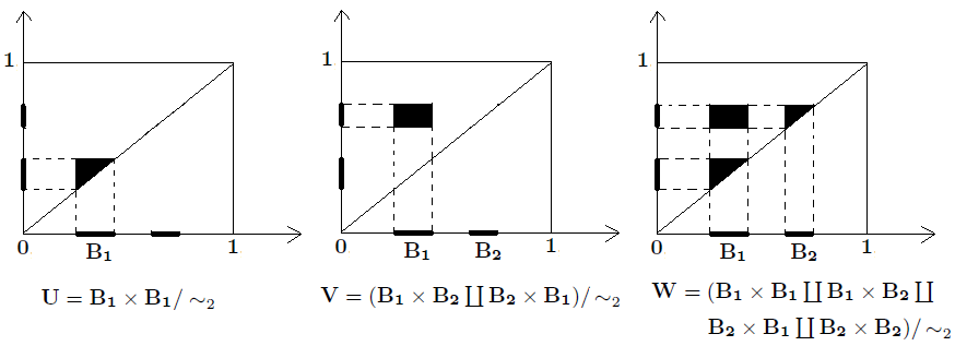 Figure 1