Hadronic Spectra from Deformed AdS Backgrounds
Eduardo Folco Capossoli, Miguel Angel Mart\'in Contreras, Danning Li,, Alfredo Vega, Henrique Boschi-Filho

TL;DR
This paper uses deformed AdS backgrounds within the AdS/CFT framework to compute hadronic spectra, including glueballs, mesons, and baryons, and compares the results with experimental data and other models.
Contribution
It introduces a method to calculate hadronic spectra using deformed AdS$_5$ spaces, deriving Regge trajectories and matching experimental data.
Findings
Glueball spectra and Regge trajectories consistent with pomeron and odderon.
Masses of scalar and vector mesons and baryons agree with PDG data.
Universal Regge slope of approximately 1.1 GeV$^2$ for various hadrons.
Abstract
Because of the presence of modified warp factors in metric tensors, we use deformed AdS spaces to apply the AdS/CFT correspondence to calculate the spectra for even and odd glueballs, scalar and vector mesons, and baryons with different spins. For the glueball cases, we derive their Regge trajectories and compare them with those related to the pomeron and the odderon. For the scalar and vector mesons as well as baryons the determined masses are compatible with the PDG. In particular for these hadrons we found Regge trajectories compatible with another holographic approach as well as with the hadronic spectroscopy, which present an universal Regge slope of approximately 1.1 GeV.
Click any figure to enlarge with its caption.
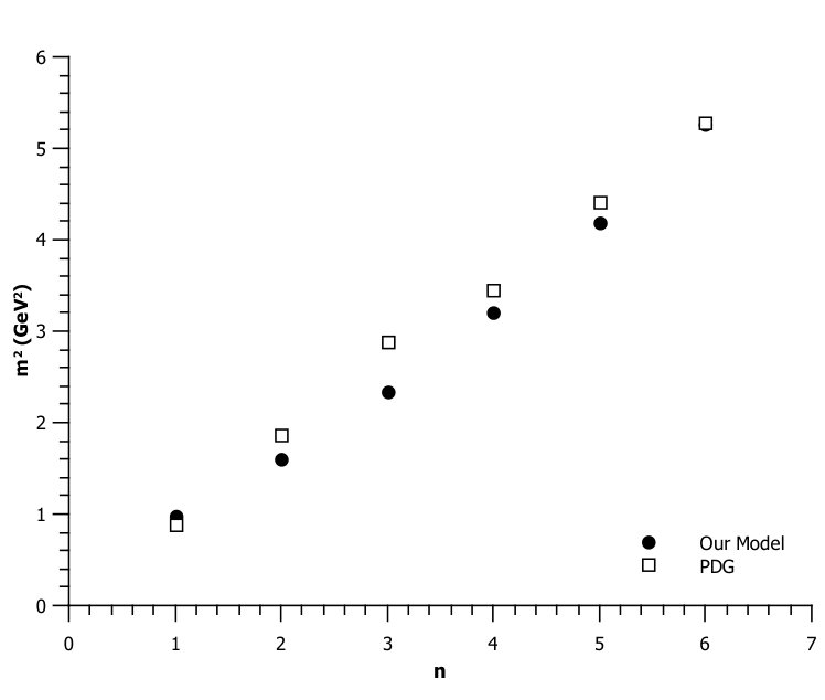 Figure 1
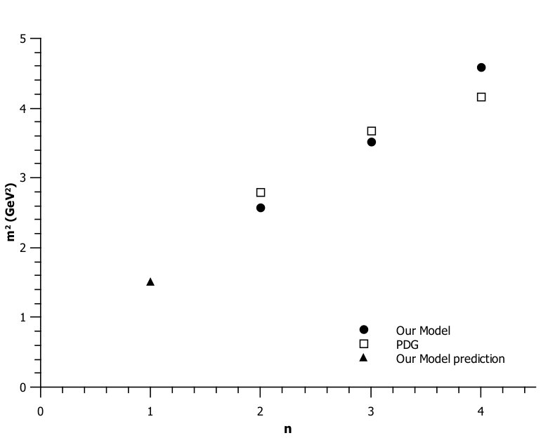 Figure 2
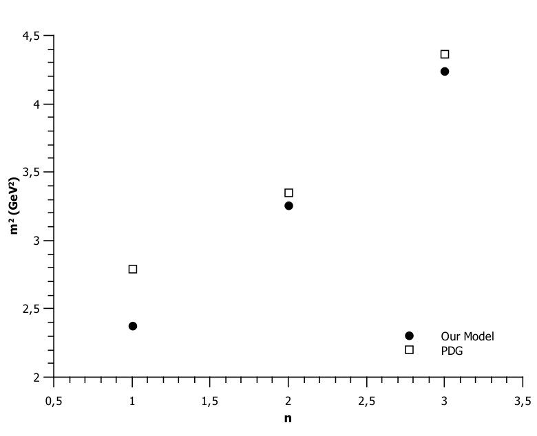 Figure 3
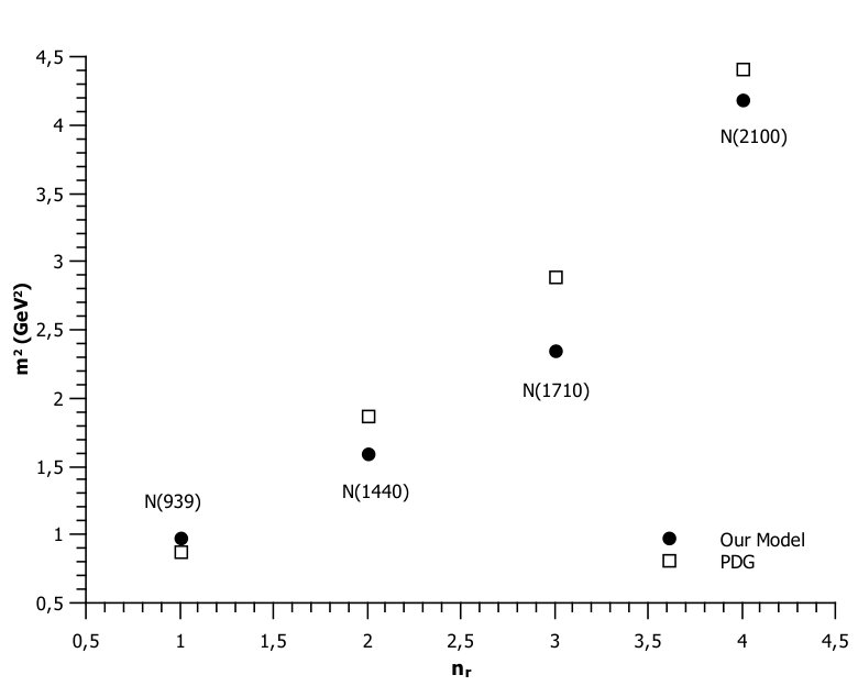 Figure 4
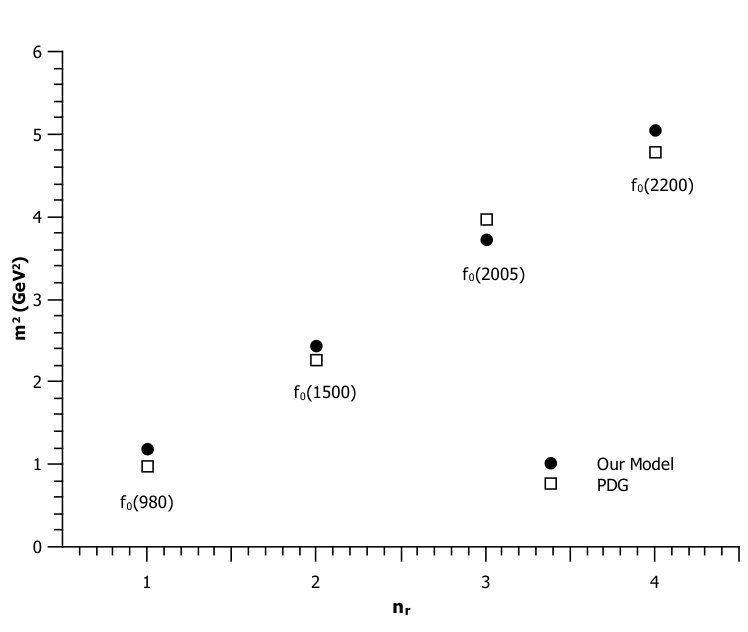 Figure 5
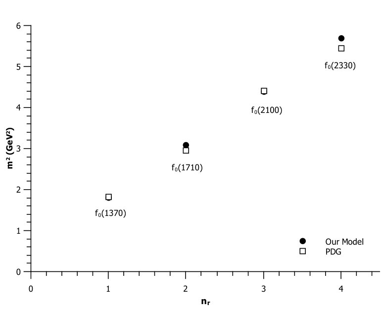 Figure 6
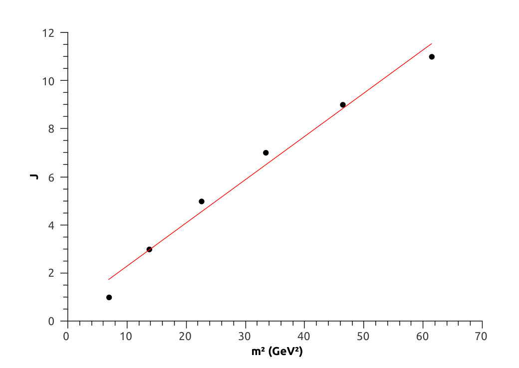 Figure 7
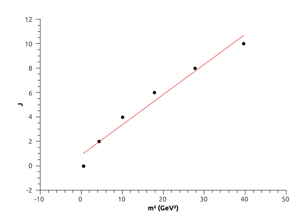 Figure 8
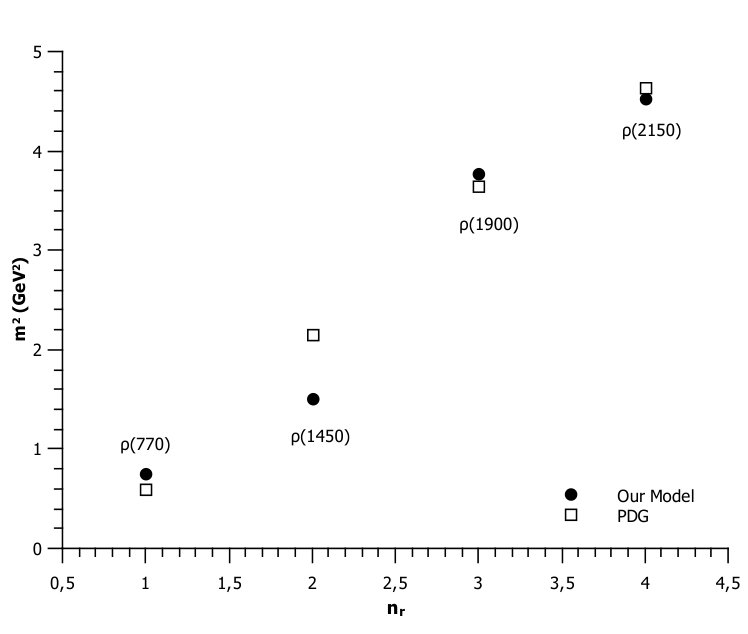 Figure 9
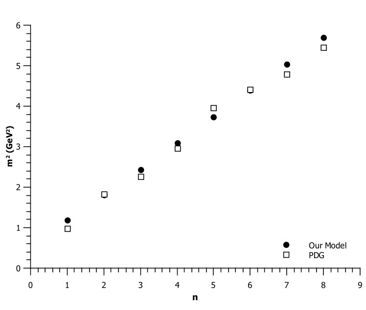 Figure 10
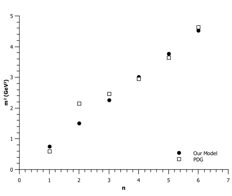 Figure 11
| Even glueball states | ||||||
| Masses | 0.76 | 2.08 | 3.17 | 4.22 | 5.26 | 6.30 |
| Odd glueball states | ||||||
| Masses | 2.63 | 3.70 | 4.74 | 5.78 | 6.81 | 7.84 |
| Models used | Even Glueball States | |||
|---|---|---|---|---|
| lattice Meyer:2004gx | 1.475(30)(65) | 2.150(30)(100) | 3.640(90)(160) | 4.360(260)(200) |
| anisotropic lattice Morningstar:1999rf | 1.730(50)(80) | 2.400(25)(120) | ||
| anisotropic lattice Chen:2005mg | 1.710(50)(80) | 2.390(30)(120) | ||
| lattice Lucini:2001ej | 1.58(11) | |||
| lattice Lucini:2001ej | 1.48(07) | |||
| Constituent models Szczepaniak:2003mr | 2.42 | 2.59 | ||
| Constituent models Mathieu:2008bf | 3.99 | 3.77 | 4.60 | |
| Models used | Odd glueball states | |||
|---|---|---|---|---|
| Relativistic many body LlanesEstrada:2005jf | 3.95 | 4.15 | 5.05 | 5.90 |
| Non-Relativistic constituent LlanesEstrada:2005jf | 3.49 | 3.92 | 5.15 | 6.14 |
| Wilson loop Kaidalov:1999yd | 3.49 | 4.03 | ||
| Vacuum correlator Kaidalov:2005kz | 3.02 | 3.49 | 4.18 | 4.96 |
| Vacuum correlator Kaidalov:2005kz | 3.32 | 3.83 | 4.59 | 5.25 |
| Semi-relativistic potential Mathieu:2008pb | 3.99 | 4.16 | 5.26 | |
| Anisotropic lattice Chen:2005mg | 3.83 | 4.20 | ||
| Isotropic lattice Meyer:2004jc ; Meyer:2004gx | 3.24 | 4.33 | ||
| Scalar meson () | ||||
|---|---|---|---|---|
| meson | GeV Tanabashi:2018oca | GeV | ||
| 1.089 | 9.97 | |||
| 1.343 | 0.54 | |||
| 1.562 | 3.87 | |||
| 1.757 | 1.96 | |||
| 1.933 | 2.96 | |||
| 2.095 | 0.27 | |||
| 2.246 | 2.61 | |||
| 2.388 | 2.17 | |||
| Vector meson )) | ||||
|---|---|---|---|---|
| meson | GeV Tanabashi:2018oca | GeV | ||
| 0.868327 | 12.0422 | |||
| 1.228 | 16.1775 | |||
| 1.50399 | 4.20467 | |||
| 1.73665 | 0.968271 | |||
| 1.94164 | 1.70972 | |||
| 2.12696 | 1.30123 | |||
| Baryons ) | ||||
|---|---|---|---|---|
| baryon | GeV Tanabashi:2018oca | GeV | ||
| 0.98683 | 5.04 | |||
| 1.264 | 7.76 | |||
| 1.531 | 9.94 | |||
| 1.791 | 3.70 | |||
| 2.046 | 2.58 | |||
| 2.296 | 0.19 | |||
| Baryons ) | ||||
|---|---|---|---|---|
| baryon | GeV Tanabashi:2018oca | GeV | ||
| 1.326 | 23.05% | |||
| 1.606 | 12.27% | |||
| 1.878 | 8.72% | |||
| Baryons ) | ||||
|---|---|---|---|---|
| baryon | GeV Tanabashi:2018oca | GeV | ||
| 1.326 | ||||
| 1.606 | 4.14 | |||
| 1.878 | 2.19 | |||
| 2.144 | 5.09 | |||
| Baryons ) | ||||
|---|---|---|---|---|
| baryon | GeV Tanabashi:2018oca | GeV | ||
| 1.542 | 7.78 | |||
| 1.804 | 1.44 | |||
| 2.059 | 1.49 | |||
Peer Reviews
No public reviews on file for this paper yet. If you reviewed it on a platform where reviews are public (OpenReview, ICLR, NeurIPS, ICML), you can paste yours below so the community can read it here.
Videos
No videos yet. Explain this paper in a talk, walkthrough, or lecture? Add one.
Hadronic Spectra from Deformed AdS Backgrounds
Eduardo Folco Capossoli1,2
Miguel Angel Martín Contreras3
Danning Li4
Alfredo Vega3
Henrique Boschi-Filho1
1Instituto de Física, Universidade Federal do Rio de Janeiro, 21.941-972 - Rio de Janeiro-RJ - Brazil
2Departamento de Física / Mestrado Profissional em Práticas da Educação Básica (MPPEB), Colégio Pedro II, 20.921-903 - Rio de Janeiro-RJ - Brazil
3Instituto de Física y Astronomía, Universidad de Valparaíso, A. Gran Bretaña 1111, Valparaíso, Chile
4Department of Physics and Siyuan Laboratory, Jinan University, Guangzhou 510632, China
Abstract
Because of the presence of modified warp factors in metric tensors, we use deformed AdS5 spaces to apply the AdS/CFT correspondence to calculate the spectra for even and odd glueballs, scalar and vector mesons, and baryons with different spins. For the glueball cases, we derive their Regge trajectories and compare them with those related to the pomeron and the odderon. For the scalar and vector mesons as well as baryons the determined masses are compatible with the PDG. In particular for these hadrons we found Regge trajectories compatible with another holographic approach as well as with the hadronic spectroscopy, which present an universal Regge slope of approximately 1.1 GeV2.
hadronic spectra, AdS/QCD model, Regge trajectories
I Introduction
Quantum Chromodynamics (QCD) is a non-Abelian quantum field theory employed for dealing with strong interactions. Although its boasts enormous success in the high energy regime, the use of QCD is difficult when investigating processes that occur at low energies (IR regions) because of the failure of the perturbative approach. This peculiar feature of the QCD is related to the fact that it is a confining theory in the IR, implying that only bound states of quarks or gluons are observed.
Hadronic spectroscopy is a highly interesting field with regard to the application of new approaches to extract information about hadronic properties, given that results are comparable with the experimental data.
Among several techniques to handle within the field of Hadronic spectroscopy, there is one that emerged in 1997 proposed by Juan Maldacena, referred to as the Anti de Sitter/Conformal Field Theory or AdS/CFT correspondence Maldacena:1997re ; Gubser:1998bc ; Witten:1998qj ; Witten:1998zw ; Aharony:1999ti . This correspondence is very useful, as it provides guidance on how to relate a weak coupling theory, which is in this case represented by a superstring theory in a ten-dimensional curved space, named with a strong coupling theory which is a super conformal Yang-Mills theory with extended supersymmetry , symmetry group in a flat four-dimensional Minkowski space.
However, the AdS/CFT correspondence cannot be used directly to reproduce QCD, as the latter is not a conformal theory, as it possesses numerous different scales (masses, critical temperature, etc.). v Some proposals appeared to break the conformal invariance and build effective theories known as AdS/QCD models, e.g, the hardwall model. In this model, the conformal symmetry is broken via introduction of a hard IR cutoff at a certain value of the holographic coordinate and by considering only a slice of the space within the interval Polchinski:2001tt ; BoschiFilho:2002vd ; BoschiFilho:2002ta . Achievements in hadronic spectroscopy within the hardwall are presented in several studies Erlich:2005qh ; DaRold:2005mxj ; deTeramond:2005su ; DaRold:2005vr ; Pomarol:2008aa ; Wang:2009wx ; Li:2013lfa .
Another example of breaking the conformal invariance is given by the softwall model. In this model a soft IR cutoff via an introduction of a dilaton field in the action. This approach was proposed in Karch:2006pv to study mesonic spectroscopy. Usually, this model is referred to as the original softwall model. Several modifications of this model were considered subsequently to deal with hadronic spectroscopy as presented in e.g., Refs. Huang:2007fv ; Vega:2008te ; Branz:2010ub ; Gutsche:2011vb ; Afonin:2012jn ; Fang:2016uer ; Cortes:2017lgz ; Contreras:2018hbi ; Afonin:2018era ; Gutsche:2019blp . Further addressing some modification in the Refs.Andreev:2006vy ; Andreev:2006ct ; Forkel:2007cm ; White:2007tu ; Bruni:2018dqm ; Rinaldi:2017wdn , instead of the introduction of a dilation in the action, a modified warp factor in the AdS metric was considered. Particularly, in Ref. Forkel:2007cm such a modification was proposed to study hadronic spectroscopy. Other modifications of the softwall model were used in Refs. Andreev:2006ct ; White:2007tu ; Bruni:2018dqm to discuss the quark-antiquark potential and in Ref. Rinaldi:2017wdn to deal with scalar and tensor glueballs. One open problem associated with the softwall model is the sign of the dilaton. In the original case, the dilaton is an exponential with a negative argument Karch:2006pv . In Refs. deTeramond:2009xk ; Zuo:2009dz ; Nicotri:2010at , authors argued that a positive dilaton is preferred, which the authors of Ref. Karch:2010eg disagree with. These authors also point out that a positive dilaton implies the existence of a massless scalar in the spectrum.
In this study, inspired by Refs. Andreev:2006vy ; Andreev:2006ct ; Forkel:2007cm , we investigate these problems with modified warp factors in the metric instead of introducing dilaton fields in the action. In this sense, in our set-up we consider deformed AdS backgrounds. Subsequently, using this approach, we compute the hadronic spectra for several particles with different spins. We employ the same form for the warp factor in the metric by fitting the free parameter in each case. The values of the parameters are observed to be different for each sector. This scenario is similar to the case of the original softwall model, where different dilaton fields are needed for each particle sector. The main advantage of our approach is that we can also directly deal with fermions, contrary to the original softwall model. Furthermore, our approach provides appropriate masses and Regge trajectories, for instance, for odd and even spin glueballs.
This paper is organized as follows. In Section II we present a brief review of the original softwall model and our deformed AdS background. In Section III, we apply our model to the even and odd spin glueball states. In Section IV, we study the case of scalar mesons obtaining their spectra. We calculate the hadronic spectra for the vector mesons in Section V and in Section VI we address the baryonic case with spins 1/2, 3/2 and 5/2. For those particles, we also obtain the corresponding Regge trajectories. In particular, for the glueballs we derive the Regge trajectories related to the pomeron and the odderon. Finally, in Section VII we present the conclusions and final comments.
II Softwall Model and Deformed AdS Set-Up
There are at least two interesting reasons behind the emergence of the softwall model. The first is related to the introduction of the soft IR cutoff instead a hard cutoff as in the hardwall model, as this approach seems more natural. The second reason lies in the fact that the softwall model truly yields linear Regge trajectories, which was an established behavior since the beginning of hadronic spectroscopy, so that
[TABLE]
where is the total angular momentum; represents the hadronic mass; (Regge slope) and are constants. The relationship between radial excitation and its squared hadron mass, given by:
[TABLE]
with and as constants.
In the original formulation of the softwall model, the action of the fields, up to some constant, is described by:
[TABLE]
where is the dilaton field, usually given by , where , and is the Lagrangian density.
The main difference between the original softwall model and the present study is the modified metric tensor using an exponential warp factor for all glueballs and hadrons. In Ref. Forkel:2007cm the authors used different warp factor profiles, usually logarithmic ones, for each hadronic sector.
As we employ the same warp factor profile in the AdS space for all glueballs and hadrons, we refer the approach of this study as a deformed background. Then, we write the deformed metric as:
[TABLE]
where is the usual AdS radius (from here onward, we assume throughout this text), is the flat Minkowski space metric tensor in four dimensions with signature , is the holographic coordinate, and for . The warp factor in Eq. (4) can be read as:
[TABLE]
In our model, the action for the fields is given as:
[TABLE]
where is the determinant of the five-dimensional metric tensor presented in Eq. (4).
III Hadronic Spectra for glueballs states
Fritzsch and Gell-Mann pointed out in Refs Dobbs:2015dwa ; Fritzsch:1972jv . “If the quark-gluon field theory indeed yields a correct description of strong interactions, there must exist glue states in the hadron spectrum”. This sentence does really reveals the importance of those “glue states” nowadays referred to as glueballs. Glueballs are colorless bound states of gluons predicted by QCD but not experimentally detected to date.
Glueballs are characterized by where (even or odd) is the total angular momentum, is the parity (spatial inversion) and is the parity (charge conjugation) eigenvalues. For the glueballs case, and .
Numerous experimental efforts were conducted in the search for glueballs Haguenauer:1993kan ; Avila:2006wy ; Ablikim:2006db ; Bai:2003ww . Some theoretical and non-holographic approaches are described in Refs. Morningstar:1999rf ; Meyer:2004jc ; Chen:2005mg ; Lucini:2001ej ; Szczepaniak:2003mr ; Mathieu:2008bf . The holographic approach is presented in Refs. BoschiFilho:2005yh ; Colangelo:2007pt ; Capossoli:2013kb ; Rodrigues:2016cdb ; BoschiFilho:2012xr ; Li:2013oda ; Capossoli:2015ywa ; Capossoli:2016kcr ; Capossoli:2016ydo ; FolcoCapossoli:2016ejd .
In this study based on a deformed AdS space, we compute the masses of even spin glueballs with and odd spin glueballs with . Even spin glueballs with are particularly interesting, as in the Chew-Frautschi plane, their states lie on the Pomeron Regge trajectory. In contrast, odd spin glueballs with lie on the odderon Regge trajectory.
We start our calculation using the standard action for a massive scalar field in space, given by:
[TABLE]
From the action (7) one can find the following equations of motion, so that:
[TABLE]
where .
The Eq. (8) can be written as:
[TABLE]
with the warp factor given in Eq. (5).
Defining , we obtain:
[TABLE]
Next, we use a plane wave ansatz with the amplitude only depending on the coordinate and propagating in the transverse coordinates with momentum ,
[TABLE]
After some algebraic manipulation and defining we obtain a “Schrödinger-like” equation:
[TABLE]
with and as eigenenergies.
III.1 Results for even and odd spin glueball spectra
To compute the glueball masses, Eq. (12) must be solved numerically. To this end, from the AdS/CFT dictionary we first relate the masses of supergravity fields in the AdS space with the scaling dimensions of an operator in the boundary theory , such that:
[TABLE]
where is the index of a form. For the case of the scalar glueball we obtain . Because the scalar glueball is dual to the fields with , its conformal dimension is .
Second, the scalar glueball state is represented on the boundary theory by the operator , given by:
[TABLE]
To raise the total angular momentum , we follow Ref. deTeramond:2005su by inserting symmetrised covariant derivatives in a given operator with spin , such that the total angular momentum after the insertion becomes . In the particular case of the operator , we obtain:
[TABLE]
with the conformal dimension . For we recover .
Thus, for even spin glueball states after the insertion of symmetrized covariant derivatives, we obtain:
[TABLE]
Hence, we write Eq.(12) as:
[TABLE]
Solving Eq.(17), for even glueball states, one obtains the four-dimensional masses presented in Table 1.
Using the data from Table 1, we plotted a Chew-Frautschi plane, here represented as , where is total angular momentum, and is the squared even glueball mass represented by the dots in figure 1. Using a standard linear regression method, we obtain the equation
[TABLE]
which represents an approximate linear Regge trajectory associated with the pomeron in agreement with Refs. Donnachie:1985iz ; Donnachie:2002en .
In contrast, for odd glueball states, the operator that describes the glueball state is given by Wang:2009wx ; Capossoli:2013kb ; Csaki:1998qr ; Brower:2000rp :
[TABLE]
where this dual operator creates odd glueball states at the boundary. This operator has the conformal dimension , and after the insertion of symmetrized covariant derivatives, we obtain:
[TABLE]
with . Therefore,
[TABLE]
and we can rewrite Eq.(12) as:
[TABLE]
Solving Eq.(22) for odd glueball states, we obtain the four-dimensional masses presented in Table 2.
Using the data in Table 2, we plotted a Chew-Frautschi plane in figure 2 for odd spin glueballs. Using a standard linear regression method, we obtain the equation
[TABLE]
which is in agreement with Ref. LlanesEstrada:2005jf , within the nonrelativistic constituent model.
Notably, the value for the constant in the warp factor for even spin glueball represented by and for odd spin glueball represented by have the same numerical value GeV2.
To facilitate the comparison between our results with the deformed AdS model and other approaches, we summarize several results provided by the literature in Tables 3 and 4.
IV Hadronic Spectra for scalar mesons
Mesons are bound states between a quark and an antiquark that can be represented by a spin singlet with total spin or a spin triplet with total spin . The coupling between and the orbital angular momentum must be considered, producing a total angular momentum in the case of the singlet state, and in the case of the triplet state.
In mesonic spectroscopy Godfrey:1998pd , mesons are characterized by , where is the isospin, is the -parity defined , and is the -parity defined for mesons as . Finally, is the -parity defined as . In the boundary theory scalar mesons are represented by the operator:
[TABLE]
where is the total angular momentum.
In this section we address light scalar mesons, i.e., and unflavored .
Within the holographic approach, the description of the scalar glueball and the scalar meson () is the same; however, the main difference is provided by the bulk mass, which defines the hadron identity. To study the scalar meson, we must to start from the action for a massive scalar field (7), which will leads us to the “Schrödinger-like” equation (12).
IV.1 Results for scalar mesons spectra
Employing the relationship , and identifying as the scalar meson bulk mass, the index of the form with the total angular momentum () for the scalar meson and depicts the conformal dimension, which is , as each quark contributes with . Finally, we rewrite Eq.(12) with as:
[TABLE]
where . Solving (25) numerically with the warp factor constant identified as GeV2, we obtain the masses compatible with the family of the scalar meson , with , as indicated in table 5. The error presented in last column of Table 5 () is the error defined by:
[TABLE]
where depicts the deviations between the data () and the model prediction (). Throughout the text, in the cases where the experimental is provided at intervals, as the state, we use the average value of the interval to evaluate the deviations. We moreover compute the total r.m.s error defined by:
[TABLE]
where and are the number of measurements and parameters, respectively. From Eq. (27) we find that for table 5.
Using the data from Table 5, we plotted a Chew-Frautschi plane represented as , where is the holographic radial excitation and, is the squared scalar meson mass represented by the dots (our model) or squares (PDG) in figure 3. Using a standard linear regression method we obtain the experimental and theoretical Regge trajectories for the scalar meson family, such that:
[TABLE]
[TABLE]
The authors of Refs. Gherghetta:2009ac ; Kelley:2011ds within a holographic softwall model likewise computed the masses for the meson family and derived its Regge trajectory slightly differently from Eq. (29). This can be explained, as the data selection scenarios in these references are different from the current study. In these past studies, the scalar meson was included, which might have caused the slight difference of the slope and the intercept compared to our study.
To connect our results with the mesonic spectroscopy data Godfrey:1998pd ; Anisovich:2000kxa ; Ebert:2009ub ; Chen:2018bbr we split the isoscalar states into two sets. The first set, i.e., set 1, is related to the states, which are represented by , , and . The second set, i.e., set 2, is related to states, also called , which is represented by , , and .
Using the states that belong to set 1 we plot a Chew-Frautschi plane represented as , where is the spectroscopy radial excitation and is the squared scalar meson mass represented by the dots (our model) or squares (PDG) in figure 4. Using a standard linear regression method we obtain the experimental and theoretical Regge trajectories for set 1, given by:
[TABLE]
[TABLE]
For the states belonging to set 2, we plot Fig. 5 and obtain the experimental and theoretical Regge trajectories, given by:
[TABLE]
[TABLE]
The Regge trajectories for scalar mesons belonging to the set 1 and 2 from our model, represented by Eqs. (31) and (33), present Regge slopes ranged within the GeV2 which is close to the universal value GeV2 Anisovich:2000kxa ; Iachello:1991re .
V Hadronic Spectra for vector mesons
Vector mesons have the same internal structure as the scalar mesons, but with total angular momentum . They are represented on the boundary theory by the operator:
[TABLE]
In the holographic description, vector mesons are dual to the massive vector field in the . Hence, the action for a massive vector field is needed, given by:
[TABLE]
where the vector field stress tensor is defined as .
The equations of motion are achieved by , so that:
[TABLE]
where .
Considering a plane wave ansatz with the amplitude only depending on the coordinate and propagating in the transverse coordinates with momentum , we obtain
[TABLE]
assuming and is the unitary vector defined in the transverse space to the coordinate, with components . We use the fact which implies ensuring that the field can be written as a plane wave. Notably that and . After some algebraic manipulation and defining , we obtain the ‘Schrödinger-like” equation, given by:
[TABLE]
where are eigenenergies.
V.1 Results for vector mesons spectra
We consider the case . Then, recalling that , and identifying as the vector meson bulk mass, the index of form as total angular momentum () for the vector meson and as the conformal dimension, which is as each quark contributes with . Finally, we rewrite Eq.(38) as:
[TABLE]
with and for vector mesons.
Solving Eq. (39) numerically with the warp factor constant given by GeV2, we obtain the masses compatible with the family of vector meson , with , as indicated in Table 6. The error presented in the last column of Table 6 () was definied in Eq.(26). We also compute the total r.m.s error defined by Eq. (27). For table 6 we obtain .
Using the data from Table 6 we plotted a Chew-Frautschi plane represented as , where is the holographic radial excitation, and is the squared vector meson mass represented by the dots (our model) or squares (PDG) in Fig. 6. Using a standard linear regression method we obtain the experimental and theoretical Regge trajectories for vector meson , such that:
[TABLE]
[TABLE]
We did not include the intercept in Eq. (41), because its value is very close to zero . Moreover, in Eq. (41), the uncertainty in the slope is very small indicating that this fit is practically a straight line.
The authors of Refs. Gherghetta:2009ac ; Kelley:2011ds also computed the masses for the meson family and derived their Regge trajectories within their holographic softwall model, obtaining approximately the same value for the slope and intercept (considering uncertainties) as the present study, Eq. (41). The data select scenarios in those studies are different from the present study, as they included the vector meson as the first radial excited state and excluded the vector meson , which the authors argue may be an OZI violating decay of the . If we assume the existence of the as the first radial excitation of the meson family, then the corresponding percentage error in Table 6 would be smaller and so would the error.
As performed for the scalar mesons, we can resort to the mesonic spectroscopy data Godfrey:1998pd ; Anisovich:2000kxa ; Ebert:2009ub ; Chen:2018bbr and note that all vector mesons listed in Table 6 are not in the same spectroscopic state, meaning that only , , and belong to the wave represented by , , and , respectively. In this study, we used the spectroscopic notation, such as, , where is the spectroscopy radial excitation. Using these states we plot in a Chew-Frautschi plane represented as , where is the spectroscopy radial excitation and is the squared vector meson mass represented by the dots (our model) or squares (PDG) in figure 7. Using a standard linear regression method, we obtain the experimental and theoretical Regge trajectories for vector meson belonging to the wave, so that:
[TABLE]
[TABLE]
The Regge trajectory for vector mesons belonging to the wave from our model, represented by Eq. (43), yield a Regge slope in the range GeV2 which is close to the universal value GeV2 Anisovich:2000kxa ; Iachello:1991re .
Furthermore, if we follow the original motivation for the softwall model, it would be natural to suppose that and are related to the string tension for the flux tube that connects the two quarks inside the meson. This information is contained in the confining part of the potential, and it is in principle a spin independent term. Therefore, in the AdS/QCD models with dilatons in the action, the slope parameter should be universal for scalar and vector mesons, as it happens in the conventional softwall model Karch:2006pv ; Colangelo:2007pt .
Interestingly and are related, namely . This peculiarity could be attributed to the fact that in the EOM for scalar mesons, Eq.(9), we performed the substitution . On the other hand, in the EOM for vector mesons, Eq.(36), we used , leading to .
VI Hadronic spectra for baryons
Within the quark model, constituent baryons are particles with a semi integer spin formed by a bound state of three valence quarks. In this study, we disregard states of baryons with higher complexity, composed of three quarks added to any number of quark and antiquark pairs, e.g., pentaquark states . Hence, we use the following description for baryons, such that:
[TABLE]
The three colors are represented by an singlet, without dynamics and completely antisymmetric. The spatial wave function is related to , and the spin-flavor wave function is related to . A review on baryon physics is provided in Refs. Klempt:2009pi ; Klempt:2002cu . In this study we are interested in light baryons composed of and quarks with a spin of 1/2 and with higher spins (3/2 and 5/2).
Within the holographic description, baryons are dual to the massive spinor fields in . We start our discussion from the free spinor field action without surface terms Henningson:1998cd ; Mueck:1998iz ; Abidin:2009hr ; Gao:2010qk :
[TABLE]
We disregarded the hypersphere , as for our purposes, the spinor field does not depend on these coordinates. Further, in the action (45), is the determinant of the metric of the deformed space, given by Eq. (4).
As we deal with fermions in a curved space, we need to construct a local Lorentz frame or a vielbein. To simplify our notation, we will use to denote indexes in flat space, and to denote indexes in curved space (deformed space). The Greek indexes are defined in the Minkowski space. Thus, a useful choice is:
[TABLE]
The Levi-Civita connection is defined as:
[TABLE]
The corresponding spin connection , is given by:
[TABLE]
Because the only non-vanishing are:
[TABLE]
we obtain:
[TABLE]
and all other components disappear.
The equations of motion are easily derived from Eq. (45), so that:
[TABLE]
Now using (4), (46) and (50), one can write the operator in (51), so that:
[TABLE]
where we employed that , , and . Here, are the usual Dirac’s gamma matrices.
The first Dirac equation in Eq. (51) assumes the following form:
[TABLE]
where , is the holographic coordinate in the AdS space and is the fermion bulk mass. Considering a solution that can be decomposed into right- and left-handed chiral components, such as:
[TABLE]
with satisfying the Dirac equation on the four-dimensional boundary space. The left and right modes also obey and .
Because the Kaluza-Klein modes are dual to the chirality spinors, we expand , so that:
[TABLE]
Using Eq. (55) with Eq. (54) in Eq. (53) we obtain a set with two coupled equations, such as:
[TABLE]
and
[TABLE]
Decoupling Eqs.(56) and (57), and performing the following change of variables
[TABLE]
we obtain a Schrödinger-like equation written for both right and left sectors, given by:
[TABLE]
where in Eqs. (59) depicts the four-dimensional fermion mass.
VI.1 Results for spin 1/2 baryons spectra
Here, we deal with light baryons with spin formed by and quarks. To this end, we consider the following operator on the boundary theory:
[TABLE]
where is the orbital angular momentum. Here we consider only the case .
From the AdS/CFT dictionary we find the following relationship for the fermion bulk mass and its conformal dimension (), so that:
[TABLE]
As each quark or contributes with , then the baryon formed by three quarks exhibits and consequently .
Replacing in the Schrödinger-like equation (59) and solving it numerically, with the warp factor constant identified as GeV2, we obtain the masses compatible with the family of baryon, with , as indicated in Table 7. The error presented in last column of Table 7 () is defined in Eq.(26). We also compute the total r.m.s error defined by Eq. (27). For Table 7 we obtain .
Using the data from Table 7, we plotted a Chew-Frautschi plane represented as , where is the holographic radial excitation and is the squared baryon mass represented by the dots (our model) or squares (PDG) in Fig. 8. Usig a standard linear regression method, we obtain the experimental and theoretical Regge trajectories for the baryon, such that:
[TABLE]
[TABLE]
As performed for the scalar and vector mesons we resort to baryonic spectroscopy and attempt to recognize which baryons among those listed in Table 7 belong to the same spectroscopy state. According to Refs. Klempt:2009pi ; Klempt:2002cu , we see that the states , , and belong to the state with spectroscopy radial excitation , corresponding to , respectively, with orbital angular momentum . In this notation, represents the 56-plet, which can be broken into an octet with spin 1/2 () and a decuplet with spin 3/2 (). For these mentioned states, we plot a Chew-Frautschi plane represented as , where is the spectroscopy radial excitation and is the squared baryon mass belonging to the state represented by the dots (our model) or squares (PDG) in Fig. 9. Using a standard linear regression method, we obtain the experimental and theoretical Regge trajectories for baryon in the state, so that:
[TABLE]
[TABLE]
The Regge trajectory for the baryon belonging to the same multiplet comes from our model, represented by Eq. (65), and presents a Regge slope in the range GeV2 which is close to the universal value GeV2 Klempt:2002vp .
VI.2 Results for higher spin baryons spectra
Here, we deal with light baryons, according to the same structure as in the previous section and a higher spin, meaning, e.g., or . To this end, we we employ the same approach for the higher spin glueball as in Subsection III.1. To obtain the spectrum for spin baryons we insert symmetrized covariant derivatives in the operator , given by Eq. (60). Then, the conformal dimensions related to the spin baryons is now , with . Solving Eq. (59) with the warp factor constant given by GeV2, we obtain the masses compatible with the family of baryon, with , as indicated in Table 8. The error presented in last column of table 8 () is defined in Eq.(26). We also compute the total r.m.s error defined by Eq. (27). For Table 9 one finds .
Observing the column in Table 8, The errors between and are excessively high, especially for and states. A possible reinterpretation would be a missing state, which represents the ground state for the baryons family. Taking into account this assumption, regarding a possible missing state, we can reinterpret Table 8 as in Table 9, where in the first line we present a possible baryon prediction obtained within the deformed AdS model. The error presented in last column of table 9 () is defined in Eq.(26), We also compute the total r.m.s error defined by Eq. (27). For table 9 we find . We excluded our prediction of the errors calculation. The error in Table 8 are greater than in Table 9. However,this possible ground state that we are reinterpreting is not found in PDG. In PDG the states with and mass around 1320 MeV, is found; hence, our model is possibly not capable to distinguishing these two states. This first state could be as both trajectories, and , are supposed to be degenerate in the chiral limit, as it happens with mesons and .
Using the data from Table 9 we plotted a Chew-Frautschi plane represented as , where is the holographic radial excitation and is the squared baryon mass represented by the dots (our model), by the triangle (our model prediction) or squares (PDG) in Fig. 10. Using a standard linear regression method we obtain the experimental and theoretical Regge trajectories for baryons, so that:
[TABLE]
[TABLE]
For the linear fit in Eq.(67) we took into account our predicted state.
The Regge trajectory for the baryon family from our model, represented by Eq. (67), present a Regge slope in the range GeV2 which is close to the universal value GeV2 Klempt:2002vp .
At this point, we deal with baryons of spin 5/2. To this end, once again, insert one more symmetrized covariant derivative in the operator given by Eq. (60). Then, we obtain the conformal dimension, given by , which provides . Solving Eq. (59) with the warp factor constant given by GeV2, we obtain the masses compatible with the family of baryons, with , as indicated in Table 10. The error presented in the last column of table 10 () is defined in Eq. (26). We compute the total r.m.s error defined by Eq. (27). For Table 10 one finds .
From Table 10, we plotted a Chew-Frautschi plane as , where is the holographic radial excitation and is the squared baryon mass represented by the dots (our model) or squares (PDG) in figure 11. Using a standard linear regression method we obtain the experimental and theoretical Regge trajectories for baryons, so that:
[TABLE]
[TABLE]
The Regge trajectory for the baryon family from our model, represented by Eq. (69), present a Regge slope near the range GeV2 which is close to the universal value GeV2 Klempt:2002vp .
Notably, the numeric values of the warp factor constant for the baryons in this study are approximately independent of their spin, meaning that .
VII Summary and conclusions
We studied the hadronic spectra based on the holographic model within deformed space metrics, establishing that the warp factor is instead of of the pure AdS space. This deformation implies that there is no dilaton field in the action as in the original softwall model. In our model, different values are needed for the parameter for each particle sector. A possible interpretation for this behavior is the following: if one assumes that the QCD vacuum is defined by the metric, our result of multiple values of indicates that the QCD vacuum should be non-trivial and possibly composed of various non-equivalent vacua states.
The main achievement of this study is to provide an approach that can adequately accommodate the spectra for even and odd glueballs, scalar () and vector mesons , as well as baryons with spin 1/2, 3/2 and 5/2 using the same holographic approach. This implies that the masses of these mentioned particles, computed using our model, and the derived Regge trajectories are in agreement with the literature.
For the even and odd glueball cases, our model provides appropriate masses, as indicated in Tables 1 and 2, when compared with other approaches (a summary of even and odd spin glueball masses obtained from lattice and other models, is given in Tables 3 and 4). The computed masses for higher even and odd spin glueballs were placed in a Chew-Frautschi plane . We derived the Regge trajectories related to the pomeron and the odderon which are likewise in agreement with the literature.
Our model performs well for scalar mesons, providing appropriate masses for the (), as indicated in Table 5, as compared with the data from PDG Tanabashi:2018oca . The obtained Regge trajectory from is compatible with the one of the holographic softwall model Gherghetta:2009ac ; Kelley:2011ds . Using spectroscopy data for the scalar mesons, we split them into two sets. The first one contains only , while the second contains only . For these sets, we derived Regge trajectories in and found that they are compatible with the literature Anisovich:2000kxa ; Iachello:1991re .
For the vector meson our model provided appropriate masses as well, as shown in Table 6 compared with PDG. The obtained Regge trajectory from is compatible with the one from the holographic softwall model Gherghetta:2009ac ; Kelley:2011ds . Using the spectroscopy data for the vector mesons, we selected the wave states and derived their Regge trajectory in finding agreement with the literature Anisovich:2000kxa ; Iachello:1991re .
Our model also provides appropriate masses for the baryon, as shown in Table 7, compared with PDG. In this case, we likewise used the baryonic spectroscopic data to select states in the same multiplet, only varying their radial excitation. From these states we derived the Regge trajectory, which was compatible with the literature Klempt:2002vp .
For the baryon, we obtained unsatisfactory results for the masses as shown in Table 8. These results can be improved by introducing a hypothetical baryonic state to occupy the ground state (Table 9). Using this assumption, the errors decrease and the derived Regge trajectory is compatible with the literature Klempt:2002vp .
Finally, for the baryon our model provides appropriate masses, as shonw in Table 10, in comparison with PDG, and the Regge trajectory is in a reasonable agreement with the literature Klempt:2002vp .
It is important to note that in our model, the form of the warp factor is the same for all studied particles, whereas the parameter is adjusted for each case. In ref. Forkel:2007cm the authors employ different warp factors for each kind of particle that is dependent on the angular momentum. In our case, for even and odd glueballs, the value of is the same, GeV2. For scalar and vector mesons, we found that , as discussed at the end of Subsection V.1. For the baryonic case, we found .
The Regge trajectories presented in this study related to hadronic spectroscopy for scalar mesons (31), (33), vector mesons (43), and baryons (65), (67), (69) point towards a universal Regge slope around GeV2 in accordance with the literature Anisovich:2000kxa ; Iachello:1991re ; Klempt:2002vp ; Bugg:2004xu .
Our model finds different signs in the exponential of the warp factor, depending on each hadronic sector. Hence the question regarding the sign of the dilaton in the original softwall model persists. Despite the different signs for different sectors, we have no massless fields in our model. This a consequence of the deformed geometry instead of the introduction of a dilaton field in the action as in the original softwall model.
Acknowledgements.
The authors would like to thank Carlos Alfonso Ballon Bayona for useful discussions, and Oleg Andreev and Song He for useful correspondence. H.B-F. would like to thank partial financial support from Conselho Nacional de Desenvolvimento Cientifíco e Tecnológico (CNPq) and Coordenação de Aperfeiçoamento de Pessoal de Nível Superior (Capes) (Brazilian Agencies). A. V. and M. A. M. C. would like to thank the financial support given by FONDECYT (Chile) under Grants No. 1180753 and No. 3180592 respectively. D.L. is supported by the National Natural Science Foundation of China (11805084), the PhD Start-up Fund of Natural Science Foundation of Guangdong Province (2018030310457) and Guangdong Pearl River Talents Plan (2017GC010480).
The reference list from the paper itself. Each links out to its DOI / PubMed record.
- 1(1) J. M. Maldacena, “The Large N limit of superconformal field theories and supergravity,” Adv. Theor. Math. Phys. 2 , 231 (1998) [hep-th/9711200].
- 2(2) S. S. Gubser, I. R. Klebanov and A. M. Polyakov, “Gauge theory correlators from noncritical string theory,” Phys. Lett. B 428 , 105 (1998) [hep-th/9802109].
- 3(3) E. Witten, “Anti-de Sitter space and holography,” Adv. Theor. Math. Phys. 2 , 253 (1998) [hep-th/9802150].
- 4(4) E. Witten, “Anti-de Sitter space, thermal phase transition, and confinement in gauge theories,” Adv. Theor. Math. Phys. 2 , 505 (1998) [hep-th/9803131].
- 5(5) O. Aharony, S. S. Gubser, J. M. Maldacena, H. Ooguri and Y. Oz, “Large N field theories, string theory and gravity,” Phys. Rept. 323 , 183 (2000) [hep-th/9905111].
- 6(6) J. Polchinski and M. J. Strassler, “Hard scattering and gauge / string duality,” Phys. Rev. Lett. 88 , 031601 (2002) [hep-th/0109174].
- 7(7) H. Boschi-Filho and N. R. F. Braga, “Gauge / string duality and scalar glueball mass ratios,” JHEP 0305 , 009 (2003) [hep-th/0212207].
- 8(8) H. Boschi-Filho and N. R. F. Braga, “QCD / string holographic mapping and glueball mass spectrum,” Eur. Phys. J. C 32 , 529 (2004) [hep-th/0209080].