Better Approximations of High Dimensional Smooth Functions by Deep Neural Networks with Rectified Power Units
Bo Li, Shanshan Tang, Haijun Yu

TL;DR
This paper demonstrates that deep neural networks with rectified power units (RePU) can approximate smooth functions more efficiently than ReLU networks, requiring smaller network sizes and offering better stability and approximation properties.
Contribution
The paper introduces a novel approach using RePU activations for better approximation of smooth functions, with constructive algorithms and theoretical analysis showing improved efficiency over ReLU networks.
Findings
RePU networks require $ ext{O}( ext{log}(1/\varepsilon))$ smaller sizes than ReLU networks for the same accuracy.
RePU networks are numerically more stable and use fewer activation functions than classical methods.
RePU networks naturally fit smooth functions involving derivatives, enhancing their application in derivative-based loss functions.
Abstract
Deep neural networks with rectified linear units (ReLU) are getting more and more popular due to their universal representation power and successful applications. Some theoretical progress regarding the approximation power of deep ReLU network for functions in Sobolev space and Korobov space have recently been made by [D. Yarotsky, Neural Network, 94:103-114, 2017] and [H. Montanelli and Q. Du, SIAM J Math. Data Sci., 1:78-92, 2019], etc. In this paper, we show that deep networks with rectified power units (RePU) can give better approximations for smooth functions than deep ReLU networks. Our analysis bases on classical polynomial approximation theory and some efficient algorithms proposed in this paper to convert polynomials into deep RePU networks of optimal size with no approximation error. Comparing to the results on ReLU networks, the sizes of RePU networks required to approximate…
Click any figure to enlarge with its caption.
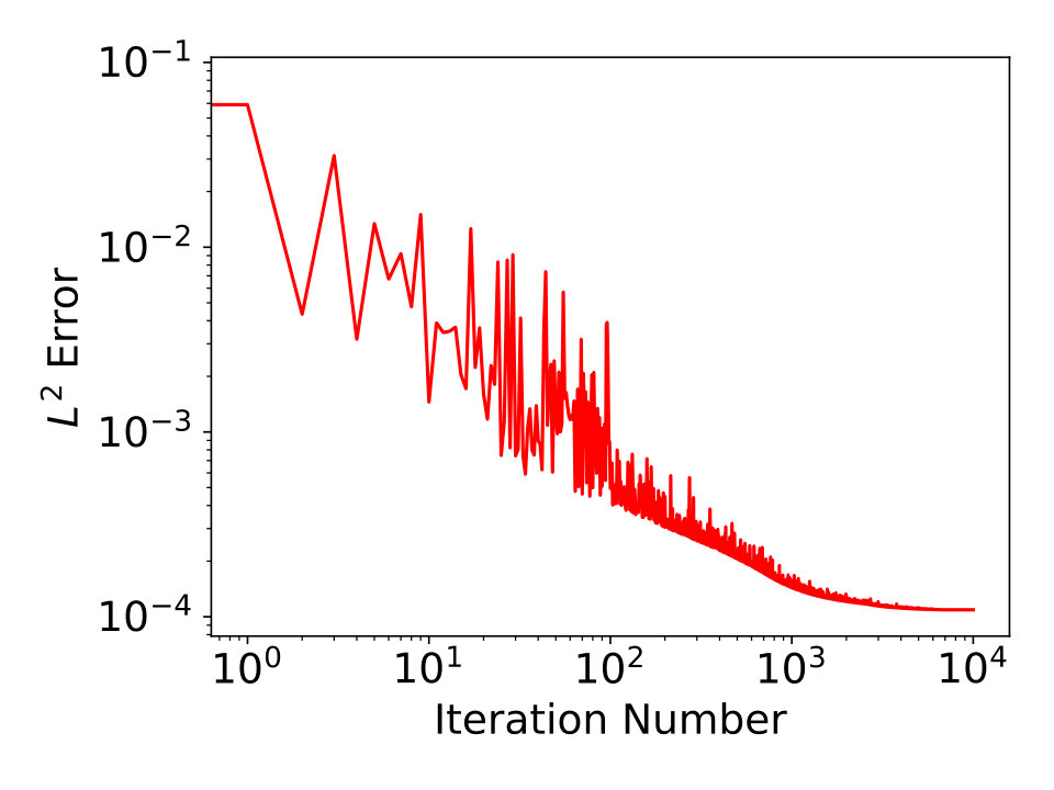 Figure 1
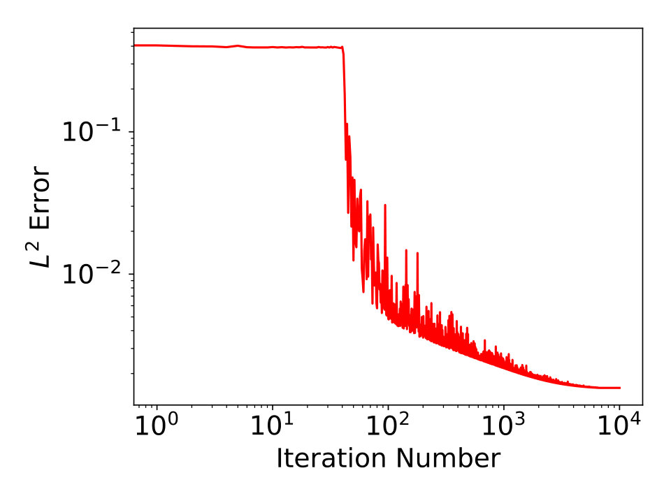 Figure 2
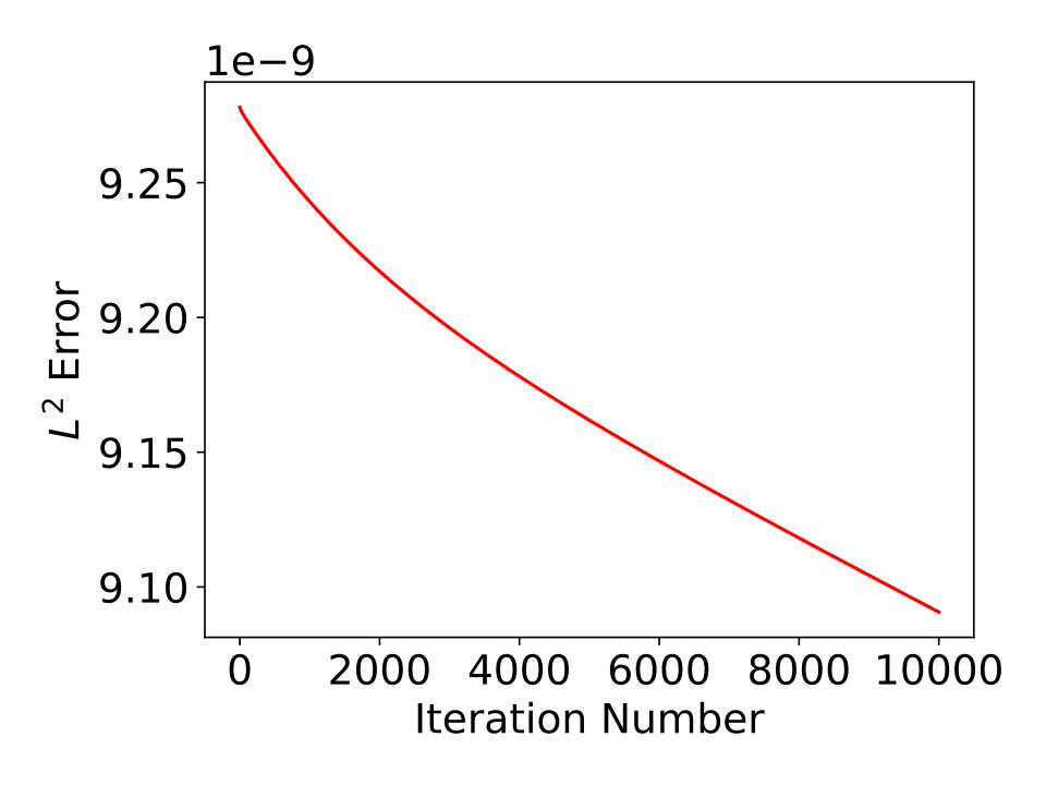 Figure 3
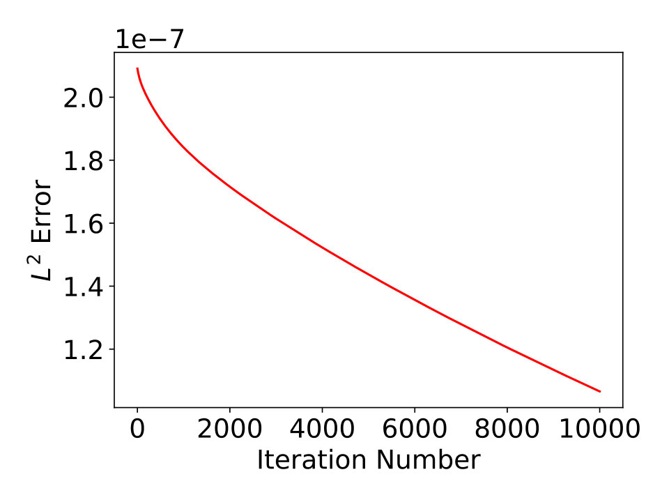 Figure 4
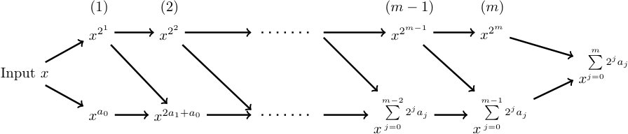 Figure 1
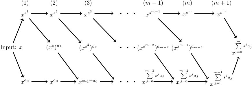 Figure 2
| Degree | -Error | |||
|---|---|---|---|---|
| 3 | 3 | 38 | 10 | 4.44e-16 |
| 7 | 4 | 64 | 15 | 2.22e-16 |
| 15 | 5 | 89 | 20 | 9.99e-16 |
| 31 | 6 | 114 | 25 | 7.77e-16 |
| 63 | 7 | 139 | 30 | 6.11e-16 |
| 127 | 8 | 164 | 35 | 2.22e-16 |
| Degree | -Error | |||
|---|---|---|---|---|
| 3 | 3 | 66 | 14 | 1.78e-15 |
| 7 | 4 | 188 | 31 | 1.78e-15 |
| 15 | 5 | 429 | 64 | 4.44e-15 |
| 31 | 6 | 910 | 129 | 5.33e-15 |
| 63 | 7 | 1871 | 258 | 5.33e-15 |
| 127 | 8 | 3792 | 515 | 5.33e-15 |
| Degree | -Error | |||
|---|---|---|---|---|
| 3 | 5 | 378 | 64 | 1.11e-15 |
| 7 | 7 | 1570 | 246 | 8.88e-15 |
| 15 | 9 | 6376 | 988 | 1.60e-14 |
| 31 | 11 | 25758 | 4002 | 7.11e-14 |
| 63 | 13 | 103668 | 16168 | 8.88e-14 |
| Degree | -Error | |||
|---|---|---|---|---|
| 7 | 7 | 1254 | 217 | 3.55e-15 |
| 15 | 9 | 3277 | 554 | 1.24e-14 |
| 31 | 11 | 8022 | 1351 | 5.32e-14 |
| 63 | 13 | 19039 | 3196 | 2.24e-14 |
| 127 | 15 | 44052 | 7393 | 4.26e-14 |
Peer Reviews
No public reviews on file for this paper yet. If you reviewed it on a platform where reviews are public (OpenReview, ICLR, NeurIPS, ICML), you can paste yours below so the community can read it here.
Videos
No videos yet. Explain this paper in a talk, walkthrough, or lecture? Add one.
00footnotetext: † The first two authors contributed equally. Author list is alphabetical.00footnotetext: ‡ The work of this author is partially done during her Ph.D. study in Academy of Mathematics and Systems Science, Chinese Academy of Sciences.
Better Approximations of High Dimensional Smooth
Functions by Deep Neural Networks with Rectified Power Units
Bo Li\comma*,†*
2
1
Shanshan Tang*,†,‡* and Haijun Yu\comma\comma\corrauth
3
1
2
11affiliationmark: NCMIS & LSEC, Institute of Computational Mathematics and Scientific/Engineering Computing, Academy of Mathematics and Systems Science, Chinese Academy of
Sciences, Beijing 100190, China
22affiliationmark: School of Mathematical Sciences, University of Chinese Academy of Sciences,
Beijing 100049, China
33affiliationmark: China Justice Big Data Institute, Beijing 100043, China
[[email protected](B. Li),
[email protected](S. Tang), [email protected](H. Yu) ](mailto:)
Abstract
Deep neural networks with rectified linear units (ReLU) are getting more and more popular due to their universal representation power and successful applications. Some theoretical progress regarding the approximation power of deep ReLU network for functions in Sobolev space and Korobov space have recently been made by [D. Yarotsky, Neural Network, 94:103-114, 2017] and [H. Montanelli and Q. Du, SIAM J Math. Data Sci., 1:78-92, 2019], etc. In this paper, we show that deep networks with rectified power units (RePU) can give better approximations for smooth functions than deep ReLU networks. Our analysis bases on classical polynomial approximation theory and some efficient algorithms proposed in this paper to convert polynomials into deep RePU networks of optimal size with no approximation error. Comparing to the results on ReLU networks, the sizes of RePU networks required to approximate functions in Sobolev space and Korobov space with an error tolerance , by our constructive proofs, are in general times smaller than the sizes of corresponding ReLU networks constructed in most of the existing literature. Comparing to the classical results of Mhaskar [Mhaskar, Adv. Comput. Math. 1:61-80, 1993], our constructions use less number of activation functions and numerically more stable, they can be served as good initials of deep RePU networks and further trained to break the limit of linear approximation theory. The functions represented by RePU networks are smooth functions, so they naturally fit in the places where derivatives are involved in the loss function.
keywords:
deep neural network, high dimensional approximation, sparse grids, rectified linear unit, rectified power unit, rectified quadratic unit
\ams
65D15, 65M12, 65M15
1 Introduction
Artificial neural network(ANN), whose origin may date back to the 1940s[1], is one of the most powerful tools in the field of machine learning. Especially, it became dominant in a lot of applications after the seminal works by Hinton et al.[2] and Bengio et al.[3] on efficient training of deep neural networks (DNNs), which pack up multi-layers of units with some nonlinear activation function. Since then, DNNs have greatly boosted the developments in different areas including image classification, speech recognition, computational chemistry and numerical solutions of high-dimensional partial differential equations and scientific problems, etc., see e.g. [4][5] [6][7][8][9][10][11][12] to name a few.
The success of DNNs relies on two facts: 1) DNN is a powerful tool for general function approximation; 2) Efficient training methods are available to find minimizers with good generalization ability. In this paper, we focus on the first fact. It is known that artificial neural networks can approximate any and functions with any given error tolerance, using only one hidden layer (see e.g. [13][14]). However, it was realized recently that deep networks have better representation power( see e.g. [15][16][17]) than shallow networks. One of the commonly used activation functions with DNN is the so called rectified linear unit (ReLU)[18], which is defined as . Telgarsky [16] gave a simple and elegant construction showing that for any , there exist -layer, wide ReLU networks on one-dimensional data, which can express a sawtooth function on with oscillations. Moreover, such a rapidly oscillating function cannot be approximated by poly-wide ReLU networks with depth. Following this approach, several other works proved that deep ReLU networks have better approximation power than shallow ReLU networks [19][20][21][22]. In particular, for -differentiable -dimensional functions, Yarotsky [21] proved that the number of parameters needed to achieve an error tolerance of is . Petersen and Voigtlaender [22] proved that for a class of -dimensional piecewise continuous functions with the discontinuous interfaces being continuous also, one can construct a ReLU neural network with layers, nonzero weights to achieve -approximation. The complexity bound is sharp. For analytic functions, E and Wang [23] proved that using ReLU networks with fixed width , to achieve an error tolerance of , the depth of the network depends on instead of itself. We also want to mention that the detailed relations between ReLU networks and linear finite elements have been studied by He et al.[24]. And recent work by Opschoor, Peterson and Schwab [25] reveals the connection between ReLU DNNs and high-order finite element methods.
One basic fact on deep ReLU networks is that function can be approximated within any error by a ReLU network having the depth, the number of weights and computation units all of order . This fact has been used by several groups (see e.g. [19][21]) to analyze the approximation property of general smooth functions using ReLU networks. In this paper, we extend the analysis to deep neural networks using rectified power units (RePUs), which are defined as
[TABLE]
where denotes the set of non-negative integers. Note that is the commonly used ReLU function, is the binary step function. We call , rectified quadratic unit (ReQU) and rectified cubic unit, respectively. We show that deep neural networks using RePUs() as activation functions have better approximation property for smooth functions than those using ReLUs. By replacing ReLU with RePU(), the functions , and can be exactly represented with no approximation error using networks having just a few nodes and nonzero weights. Based on this, we build efficient algorithms to explicitly convert functions from a polynomial space into RePU networks having approximately the same number of coefficients. This allows us to obtain a better upper bound of the best neural network approximation for general smooth functions using classical polynomial approximation theories. Note that networks have been used in the classic works by Mhaskar and his coworkers (see e.g. [26] [27][28]), where by converting spline approximations into DNNs, quasi-optimal theoretical upper bounds of function approximation are obtained. However, their constructions of neural network are not optimal for very smooth functions (the case ), the error bound obtained is quasi-optimal due to an extra factor, where is related to the smoothness of the underlying functions. Meanwhile no numerically efficient and stable algorithm is presented. In this paper, we present numerically stable and efficient constructions of RePU network representation of polynomials which result in RePU network of different structure and remove the extra factor in the approximation bounds. After this paper is put on arXiv, the RePU networks and our optimal network constructions are adopted by other authors, e.g., by using RePU networks instead of ReLU networks, a sharper bound for approximating holomorphic maps in high dimension is obtained by Opschoor, Schwab and Zech [29].
For high dimensional problems, to be tractable, the intrinsic dimension usually do not grow as fast as the observation dimension. In other words, the problems have low dimensional structure. A particular example is the class of high-dimensional smooth functions with bounded mixed derivatives, for which sparse grid (or hyperbolic cross) approximation is a very popular approximation tool [30][31][32][33][34]. In the past few decades, sparse grid method and hyperbolic cross approximations have found many applications, such as numerical integration and interpolation [30][35][36],[37], solving partial differential equations (PDE) [38] [39] [40][41][42][43], computational chemistry [32] [44][45][46], uncertainty quantification [47][48][49], etc. For high dimensional problem, we will derive upper bounds of RePU DNN approximation error by converting sparse grid and hyperbolic cross spectral approximation into RePU networks. Our work is inspired by the recent work of Montanelli and Du [50], where the connection between linear finite element sparse grids and deep ReLU neural networks is established. In this paper, we approximate multivariate functions in high order Korobov space using sparse grid Chebyshev interpolation [36] for the interpolation problem, and using hyperbolic cross spectral approximation for the projection problem [33][40]. Then, we convert the high-dimensional polynomial approximations into ReQU networks, instead of ReLU networks, to avoid adding an extra factor in the size of the neural network.
In summary, we find that RePU networks have the following good properties:
- •
RePU neural networks provide better approximations for sufficient smooth functions comparing to ReLU neural network approximations. To achieve same accuracy, the RePU network approximation we constructed needs less number of layers and smaller network size than existing ReLU neural network approximations. For example, for a function with all the partial derivatives bounded uniformly independent of derivative order, we can construct a ReQU network with no more than layers, and no more than \mathcal{O}\big{(}\frac{\log\left(1/\varepsilon\right)}{\log(\log 1/\varepsilon)}\big{)} nonzero weights to approximate it with error . More results are given in Theorem 2.12, 3.4, 4.4.
- •
The functions represented by RePU() networks are smooth functions, so they naturally fit in the places where derivatives are involved in the loss function.
- •
Compared to other high-order differentiable activation functions, such as logistic, , softplus, sinc etc., RePUs are more efficient in terms of number of arithmetic operations needed to evaluate, especially the rectified quadratic unit.
Based on the facts above, we advocate the use of deep RePU networks in places where the functions to be approximated are smooth.
The remaining part of this paper is organized as follows. In Section 2, we first show how to approximate univariate smooth functions using RePU networks by converting best polynomial approximations into RePU networks. Then we use a similar approach to analyze the ReQU network approximation for multivariate functions in weighted Sobolev space in Section 3. After that, we show how high-dimensional functions with sparse polynomial approximations can be well approximated by ReQU networks in Section 4. Some preliminary numerical results are given in Section 5. We end the paper by a short summary in Section 6.
2 Approximation of univariate functions by deep RePU networks
We first introduce some notations related to neural networks. Denote by the set of all positive integers, . Given , we denote a neural network with input of dimension , number of layer , by a matrix-vector sequence
[TABLE]
where , , are matrices, and . If is a neural network, and is an arbitrary activation function, then define
[TABLE]
where is given as
[TABLE]
and
[TABLE]
We use three quantities to measure the complexity of the neural network: number of hidden layers, number of nodes (i.e. activation units), and number of nonzero weights, which are , and number of non-zeros in , respectively, for the neural network defined in (2). For convenience, we denote by the number of nonzero components in for a given matrix or vector . For the neural network defined in (2), we also denote its number of nonzero weights as .
In this paper we study the approximation property of smooth functions by deep neural networks with RePUs as activation units. It seems that networks were first used in the classic works by Mhaskar and his coworkers (see e.g. [26], [27]) to obtain high-order convergence of neural network approximation. is also a special case of piece-wise polynomial activation function, which has been studied in [51] for shallow network approximation. We also note that has been used in a deep Ritz method proposed recently to solve PDEs using variational form [52].
The construction of RePU networks adopted by Mhaskar bases on the fact that a polynomial of degree in dimension can be represented by a linear combination of number of monomials of the form \big{(}Ax+b\big{)}^{n}, with each one using different affine transform. To represent a polynomial of degree using neural network, they first compose for times, which result in . Then a neural network with one-layer units of amount is capable to accurately represent any polynomial of degree . This kind of construction give an optimal linear approximation result for neural network using high order (the order is ) sigmoidal activation functions. However, if regard the constructed neural network as a neural network, it has hidden layers. The corresponding linear approximation bound is quasi-optimal due to this factor . Moreover, to find the corresponding network coefficients to represent a given polynomial, one needs to solve a Vandermonde-like matrix, whose condition number is known grows geometrically (see e.g. [53]). In this paper, we propose a different approach which does not involve any Vandermonde matrix of large size.
2.1 Approximation by deep ReQU networks
Our analyses relies upon the fact: , , , , and all can be realized by neural networks with a few number of coefficients. We first give the result for case.
Lemma 2.1**.**
For any , the following identities hold:
[TABLE]
where
[TABLE]
If both and are non-negative, the formula for and can be simplified to the following form
[TABLE]
where
[TABLE]
Proof 2.2**.**
All the identities can be obtained by straightforward calculations.
Note that the realizations given in Lemma 2.1 are not unique. For example, to realize , we may use
[TABLE]
for general , and use
[TABLE]
for non-negative . To have a neat presentation, we will use (5)-(11) throughout this paper even though simpler realizations may exist for some special cases. We notice that the realization of the identity map given in (6) is a special case of with . Furthermore, the constant function can be represented by a trivial network with and .
Remark 2.3**.**
Notice that in [21, 22, 50], all the analyses rely on the fact that can be approximated to an error tolerance by a deep ReLU networks of complexity . In our approach, by replacing ReLU with ReQU, is represented with no error using a ReQU network with only one hidden layer and 2 hidden neurons. This simple replacement greatly simplifies the proofs of some existing deep neural network approximation bounds, improves the approximation rate and meanwhile reduces the network complexity.
2.1.1 Optimal realizations of polynomials by deep ReQU networks with no error
The basic property of given in Lemma 2.1 can be used to construct deep neural network representations of monomials and polynomials. We first show that the monomial can be represented exactly by deep ReQU networks of finite size but not shallow ReQU networks.
Theorem 2.4**.**
A) The monomial defined on can be represented exactly by a network. The number of network layers, number of hidden nodes and number of nonzero weights required to realize are at most , and , respectively. Here represents the largest integer not exceeding for .
B) For any , can not be represented exactly by any ReQU network with less than hidden layers.
Proof 2.5**.**
1) We first prove part B. For a one-layer ReQU network with activation units, one input and one output, the function represented by the network can be written as
[TABLE]
where and , are the parameters of the network. Obviously, is a piecewise polynomial with at most pieces in the intervals divided by distinct points of , (suppose the points are in ascending order). In each piece, is a polynomials of degree 2. Since a polynomial of degree at most 2 composed with another polynomial of degree at most 2 produces a polynomial of degree at most 4, so a ReQU network with two hidden layers can only represent piecewise polynomials of degree at most 4. By induction, a ReQU network with hidden layers can only represent piecewise polynomials of degree at most . So, with , a ReQU network with hidden layers can’t exactly represent .
2) Now we give a constructive proof for part A. We first express in binary system as follows:
[TABLE]
where for , , and . Then
[TABLE]
Introducing intermediate variables
[TABLE]
then
[TABLE]
We use the iteration scheme
[TABLE]
and (12) to realize . The outline of the realization is demonstrated in Fig. 1. In each iteration step, we need to realize two basic operations: and , where stands for respectively. Note that can be realized by Eqs. (5) and (9) in Lemma 2.1. For the operation , since , by (7), we have
[TABLE]
where .
Now we describe the procedure in detail. For , we follow the idea given in Eq. (13) and Fig. 1. The function is realized in steps, which are discussed below.
In Step , we calculate
[TABLE]
which implies the first layer output of the neural network is:
[TABLE]
and
[TABLE]
Since , , , it is easy to see that the number of nodes in the first hidden layer is , and the number of non-zeros is: . 2. 2)
In Step , , we calculate
[TABLE]
which suggest the -th layer output of the neural network is:
[TABLE]
and
[TABLE]
We have
[TABLE]
By a direct calculation, we find that the number of nodes in Layer is , and the number of non-zeros in Layer , is . For , . 3. 3)
In Step , we calculate
[TABLE]
which implies
[TABLE]
So we get , with
[TABLE]
and
[TABLE]
By a direct calculation, we get the number of nodes in Layer is , the number of non-zero weights is .
For Layer , which is the output layer of the overall network, , and . There are no activation units and the number of nonzero weights is .
The ReQU network we just built has layers. The total number of nodes is . The total number of nonzero weights is . Combining the cases , we reach to the desired conclusion.
Now we consider how to convert univariate polynomials into networks. If we directly apply Theorem 2.4 to each monomial term in a polynomial and then combine them together, one would obtain a network of depth and size , which is not optimal. We provide here two algorithms to convert a polynomial into a ReQU network of same scale, i.e. without the extra factor. The first algorithm is a direct implementation of Horner’s method (also known as Qin Jiushao’s algorithm in China):
[TABLE]
To describe the algorithm iteratively, we introduce the following intermediate variables
[TABLE]
Then we have . By implementing of for each , using the realizations formula given in Lemma 2.1, and stacking the implementations of steps up, we obtain a neural network with layers and where each layer has a constant width independent of .
The second construction given in the following theorem can achieve same representation power with same amount of weights but much less layers.
Theorem 2.6**.**
If is a polynomial of degree on , then it can be represented exactly by a neural network with hidden layers, and the numbers of nodes and nonzero weights are both of order . To be more precise, the number of nodes is bounded by , and number of nonzero weights is bounded by .
Proof 2.7**.**
Assume , . We first use an example with to demonstrate the process of network construction as follows:
[TABLE]
Here , , and , are the intermediate variable output of Layer , , , respectively. The final output is .
We first describe the construction for the case here.
Denote . We first extend to include monomials up to degree by zero padding:
[TABLE]
The process of building a network to represent is similar to the case . We give details below.
The output of Layer intermediate variables are:
[TABLE]
which suggest
[TABLE]
and
[TABLE]
with , , . 2. 2)
The output of Layer intermediate variables are:
[TABLE]
which imply
[TABLE]
and most elements in are zeros. The nonzero elements are given below using a Matlab subscript style as:
[TABLE]
for , and the last element of is . According to the result (33) of Layer , we get
[TABLE]
We also have
[TABLE]
Here , and is the identity matrix in . stands for Kronecker product. 3. 3)
The output of Layer intermediate variables are:
[TABLE]
Denote . We have
[TABLE]
where have the same formula as given in (37) except that the maximum value of is rather than , and has the same formula as given in (39) with replaced by and . Combining (42) and (39), we get
[TABLE] 4. 4)
The output of Layer intermediate variables are:
[TABLE]
Written into the following form
[TABLE]
we have
[TABLE]
and
[TABLE]
The iteration formula for is , where
[TABLE] 5. 5)
Since , the network ends at Layer , with . So we get , and from Eq. (45).
For , the procedure can be obtained by removing some sub-steps from the cases . From the construction process, we see that the number of layers is , the numbers of nodes in Layer 1 to Layer are , and 8 respectively, and the number of nonzero weights in , are not bigger than 10, , , 72, 8 respectively. Summing up these numbers, we reach the desired bound.
Remark 2.8**.**
Theorem 2.4 says we can use a network of scale to represent exactly. Theorem 2.6 says that any polynomial of degree less than can be represented exactly by a neural network with hidden layers, and no more than nonzero weights. Such results are not available for ReLU network and neural networks using other non-polynomial activation functions, such as , , , etc. We note that the constants in the two theorems may not be optimal, but the orders of number of layers and number of nonzero weights are optimal.
2.1.2 Error bounds of approximating smooth functions by
deep ReQU networks
Now we analyze the error of approximating general smooth functions using ReQU networks. We first introduce some notations and give a brief review of some classical results of polynomial approximation.
Let be the domain on which the function to be approximated is defined. For the 1-dimensional case in this section, we focus on . Similar discussions and results can be extended to and as well. We denote the set of polynomials with degree up to defined on by , or simply . Let be the Jacobi polynomial of degree , ; the family of all these polynomials forms a complete set of orthogonal bases in the weighted space with respect to weight for . To describe functions with high order regularity, we define the Jacobi-weighted Sobolev space as (see e.g. [54]):
[TABLE]
with norm
[TABLE]
Define the -orthogonal projection : by requiring
[TABLE]
A detailed error estimate on the projection error is given in Theorem 3.35 of [54], by which we have the following theorem on the approximation error of ReQU networks.
Theorem 2.9**.**
Let , . For any , there exist a ReQU network with hidden layers, nodes, and nonzero weights, satisfying the following estimates.
1) If , we have
[TABLE]
2) If , we have
[TABLE]
Here for .
Proof 2.10**.**
For any given , the polynomial . The projection error is estimated by Theorem 3.35 in [54], which is (52) and (53) with replaced by . By Theorem 2.6, can be represented exactly by a ReQU network with hidden layers, nodes, and nonzero weights, i.e. . We thus obtain estimation (52) and (53).
Remark 2.11**.**
In (52) and (53), we allow the error measured in high-order derivatives, i.e. , because is an exact realization of a polynomial, which is infinitely differentiable. In practice, if is a trained network with numerical error, we can not measure the error with derivatives order , since is not in space.
Based on Theorem 2.9, we can analyze the network complexity of -approximation of a given function with certain smoothness. For simplicity, we only consider the case with . The result is given in the following theorem.
Theorem 2.12**.**
For any given function with norm less than , where is either a fixed positive integer or infinity, and for small enough, there exists a ReQU network with number of layers , number of nonzero weights satisfying
- •
if is a fixed positive integer, then , and N=\mathcal{O}\big{(}{\varepsilon}^{-\frac{1}{m}}\big{)};
- •
if , i.e. , then , and ,
that approximates within an error tolerance , i.e.
[TABLE]
Proof 2.13**.**
For a fixed , or , we obtain from (52) that
[TABLE]
By above estimate, we obtain that to achieve an error tolerance to approximate a function with norm less than , it suffices to take . For fixed , we have N=\mathcal{O}\big{(}{\varepsilon}^{-\frac{1}{m}}\big{)}, the depth of the corresponding ReQU network is .
For , by taking in Theorem 2.9, we have
[TABLE]
where is a general constant, and can be larger than any fixed positive number for sufficient large . To approximate a function with norm less than with error , it suffices to take , which means . The depth of the corresponding ReQU network is . Here is assumed to be small enough such that \log_{2}\big{(}\log\frac{c^{\prime}}{\varepsilon}\big{)} is no less than 1.
2.2 Approximation by deep networks using general rectified power units
The results of approximation monomials, polynomials and general smooth functions by ReQU networks discussed in Subsection 2.1 can be extended to general RePU networks.
To keep the paper short, we only present the results on approximating monomials with RePU in Theorem 2.14. The other results similar to ReQU networks can be obtained but the details are quite lengthy, we report them in a separate paper [55].
Theorem 2.14**.**
Regarding the problem of using neural networks to exactly represent monomial , , we have the following results:
- (1)
If , the monomial can be realized exactly using a networks having only 1 hidden layer with two nodes.
- (2)
If , the monomial can be realized exactly using a networks having only 1 hidden layer with no more than nodes.
- (3)
If , the monomial can be realized exactly using a networks having hidden layers with no more than nodes, no more than nonzero weights.
Proof 2.15**.**
(1) It is easy to check that has an exact realization given by
[TABLE]
(2) For the case of , we consider the following linear combination
[TABLE]
where , are parameters to be determined. are binomial coefficients. The above expression is equal to , provided that the parameters solve the following linear system:
[TABLE]
where the top-left submatrix of is a Vandermonde matrix, which is invertible as long as , are distinct. For simplicity, we choose , to be equidistant points, then (59) is uniquely solvable. Solving for we obtain an exact representation of using (58), which corresponds to a neural network having one hidden layer with no more than units.
For example, when , we may take , . Solving Eq. (59) with , we get , , and . Thus
[TABLE]
When , take , , , we obtain
[TABLE]
(3) Now, we consider the case , . For any given numbers , using the identity
[TABLE]
and the fact that , both can be realized exactly by a one layer network with no more than nodes, we conclude that the product can be realized by one layer network with no more than nodes. To realize by , we rewrite in the following form
[TABLE]
where for and . So we have
[TABLE]
Define , , , and
[TABLE]
we have . Eq. (63) can be regarded as an iteration scheme, with iteration variables , where the subscript stands for the iteration step. A schematic diagram for this iteration is given in Fig. 2. Different to Theorem 2.4, for , we need a deep neural network with hidden layers to realize , due to the introduction of intermediate variables . In each layer, we need no more than activation nodes to calculate , , and . So in total we need no more than nodes. A direct calculation shows that the number of nonzero weights in the network is no more than . The theorem is proved.
3 Approximation of multivariate functions
In this section, we discuss how to approximate multivariate smooth functions by ReQU networks. Similar to the univariate case, we first study the representation of polynomials then discuss the approximation error of general smooth functions.
3.1 Deep ReQU network representations of multivariate polynomials
Theorem 3.1**.**
If is a multivariate polynomial with total degree on , then there exists a neural network having hidden layers with no more than activation functions and nonzero weights, that can represent with no error. We note that, here the constant behind the big can be bounded independent of .
Proof 3.2**.**
1) We first consider the 2-dimensional case. Suppose and (the results for are similar but easier, so skipped here). To represent exactly with a neural network based on the results for the 1-dimensional case given in Theorem 2.6, we first rewrite as
[TABLE]
So to realize , we can first realize , using small networks , , i.e. for given input ; then use a network to realize the 1-dimensional polynomials . There are two places that need some technical treatment, the details are given below.
- (1)
The network takes , and as input. So these quantities must be presented at the same layer of the overall neural network, because we do not want connections over non-adjacent layers. By Theorem 2.6, the largest depth of networks , is , so we can lift to layer using multiple operations. Similarly, we also keep a record of input in each layer using multiple operations, such that , can start from appropriate layer and generate output exactly at layer . The overall cost for recording in layers is , which is small comparing to the number of coefficients . 2. (2)
While realizing , the coefficients are network input instead of fixed parameters. So when applying the network construction given in Theorem 2.6, we need to modify the structure of the first layer of the network. More precisely, Eq. (30) in Theorem 2.6 should be changed to
[TABLE]
So the number of nodes for the first layer changed from to , the number of nonzero weights for the first layer changed from to . So the number of hidden layers, number of nodes and nonzero weights of can be bounded by , , and respectively.
Assembling , the overall network to represent has layers with number of nodes no more than
[TABLE]
and number of weights no more than
[TABLE]
Thus, we proved that the theorem is true for the case .
2) The case can be proved by mathematical induction using the similar procedure as done for case. Note that we pad in some zeros in each direction in the iteration. Since after each dimension iteration, the number of degree of freedom are geometrically reduced, by a straightforward calculation, one can show that the constant behind the big can be made independent of dimension . An improved algorithm using less padding zeros is proposed in another paper [55].
Using a similar approach as in Theorem 3.1, one can easily prove the following theorem.
Theorem 3.3**.**
For a polynomial in a tensor product space , there exists a network having hidden layers with no more than activation functions and nonzero weights, can represent with no error.
3.2 Error bounds of approximating multivariate
functions by ReQU networks
Now we analyze the error of approximating general multivariate smooth functions using ReQU networks.
For a vector , we define , . Define the high dimensional Jacobi weight as . We define the multidimensional Jacobi-weighted Sobolev space as [54]:
[TABLE]
with norm and semi-norm
[TABLE]
Define the -orthogonal projection : by the property
[TABLE]
Then for , we have the following error estimate (see Theorem 8.1 and Remark 8.13 in [54]):
[TABLE]
where is an absolute constant. Combining (67) and Theorem 3.3, we obtain the following upper bound for the -approximation of functions in space.
Theorem 3.4**.**
For any , with , and any there exists a neural network having layers with no more than nodes and nonzero weights, that approximates with -error less than , i.e.
[TABLE]
Remark 3.5**.**
According to the classic nonlinear approximation theory by DeVore, Howard and Micchelli [56], the results of Theorem 2.12 (first part) and Theorem 3.4 are optimal in the case that the approximation depends on the function to be approximated continuously.
Remark 3.6**.**
Note that results for approximating functions in weighted Sobolev space given in Theorem 3.4 can be extended to if is sufficient large, similar to the second part of Theorem 2.12. Comparing this result with Theorem 1 in [21], we see that the number of computational units and nonzero weights needed by a ReQU network to approximate a function for sufficient large, with an error tolerance is less than that needed by a ReLU network. The ReLU network is times larger than corresponding ReQU network. For low accuracy approximation, the factor is not very big, but for high accuracy approximations, this factor can be as large as several dozens, which could make a big difference in large scale computations.
Note that, for functions with fixed lower order continuity, ReLU network can give good approximation using less number of layers, or use very deep ReLU networks to break the bounds given in Theorem 3.4. We refer interested readers to the recent works by Voigtlaender and Petersen [57], and Yarotsky [58].
4 High-dimensional functions with sparse
polynomial
approximations
In last section, we showed that for a -dimensional function with partial derivatives up to order in can be approximated within error by a ReQU neural network with complexity . When is fixed or much smaller than , the network complexity has an exponential dependence on . However, in a lot of applications, high-dimensional problems may have low intrinsic dimension (see e.g. [59][60]). One particular example are high-dimensional tensor product functions(or linear combinations of finite terms of tensor product functions), which can be well approximated by a hyperbolic cross or sparse grid truncated series.
4.1 A brief review of hyperbolic cross approximations and sparse grids
Sparse grids were originally introduced by S. A. Smolyak[30] to integrate or interpolate high dimensional functions. Hyperbolic cross approximation is a technique similar to sparse grids but without the concept of grids. We introduce hyperbolic cross approximation by considering a tensor product function: . Suppose that have similar regularity that can be well approximated by using an orthonormal bases ; that is,
[TABLE]
where is a general constant, is a constant depending on the regularity of , . So we have an expansion for as
[TABLE]
where
[TABLE]
Thus, to have a best approximation of using finite terms, one should take
[TABLE]
where
[TABLE]
is the hyperbolic cross index set. We call defined by (69) a hyperbolic cross approximation of .
For general functions defined on , we choose to be multivariate Jacobi polynomials , and define the hyperbolic cross polynomial space as
[TABLE]
Note that the definition of doesn’t depend and . is used to served as a set of bases for . To study the error of hyperbolic cross approximation, we define Jacobi-weighted Korobov-type space
[TABLE]
with norm and semi-norm
[TABLE]
For any given , the hyperbolic cross approximation can be defined as a projection by requiring
[TABLE]
Then we have the following error estimate about the hyperbolic cross approximation (see Theorem 2.2 in [33]):
[TABLE]
where is a constant independent of . It is known that the cardinality of is of order in [33]. The above error estimate says that to approximate a function with an error tolerance , one only needs a space of Jacobi polynomials of dimension at most , the exponential dependence on is weakened (cp. Theorem 3.4). To remove the exponential term , one may consider a more general sparse polynomial space[33]:
[TABLE]
In particular, is the hyperbolic cross space defined in (71), and X^{d}_{N,-\infty}:=\text{span}\big{\{}\,J_{\bm{n}}^{\bm{\alpha},\bm{\beta}},\ |\bm{n}|_{\infty}\leq N\,\big{\}} is the standard full grid. For , it is known that (see lemma 3 in [32]):
[TABLE]
where is a constant that depends on and but is independent of . We call optimized hyperbolic cross polynomial space. It is proved by Shen and Wang that the -orthogonal projection from Korobov space to satisfies the following estimate (see Theorem 2.3 in [33]):
[TABLE]
where is a constant independent of . From (77) and (78), we get that to approximate a function with an error tolerance , one only needs a space of Jacobi polynomials of dimension at most . We will later use this estimate to derive another upper bound of approximating functions in using deep ReQU networks.
In practice, the exact hyperbolic cross projection is not easy to calculate. An alternate approach is the sparse grid, which uses hierarchical interpolation schemes to build a hyperbolic cross-like approximation of high dimensional functions. To define sparse grids for , we first define the underlying 1-dimensional interpolations. Given a series of interpolation point sets , , , with , the interpolation on for is defined as
[TABLE]
where are the Lagrange interpolation polynomials for the interpolation points . The sparse grid interpolation for high-dimension function is defined as [30]:
[TABLE]
where , . For convenience, we define , , . Formally, (80) can be defined on any grids . However, to have a one-to-one transform between the values on interpolation points and the coefficients of linearly independent bases in the interpolation space, we need to be nested, i.e. . Fast transforms between physical values and interpolation coefficients always exist for sparse grid interpolations using nested grids [40, 41]. Define sparse grid index set as
[TABLE]
Then the set of the sparse grid interpolation points and the corresponding interpolation space are given as
[TABLE]
[TABLE]
where can be chosen as the hierarchical interpolation basis defined in [40], or the Lagrange-type -dimensional interpolation polynomial on points , which takes value on -th interpolation point and [math] on the other points.
A commonly used 1-dimensional scheme is the Chebyshev-Gauss-Lobatto scheme, which uses the extrema of the Chebyshev polynomials as interpolation points:
[TABLE]
In order to obtain nested sets of points, are chosen as
[TABLE]
with . Define
[TABLE]
Then for any function , with , the interpolation error on the above Chebyshev sparse grids are bounded as Theorem 8 in [36]:
[TABLE]
where is the number of points in the sparse grids, and is a constant that depends on only. Note that if a different norm instead of the norm is used, one can improve the result a little bit, but no results with error bound smaller than is known.
4.2 Error bounds of deep ReQU network approximation for
multivariate
functions with sparse structures
Now we discuss the ReQU network approximation of high-dimensional smooth functions with sparse polynomial expansions, which takes hyperbolic cross and sparse grid polynomial expansions as examples. We introduce the concept of downward closed polynomial space first. A linear polynomial space is said to be downward closed if it satisfies the following: if -dimensional polynomial , then for any , at the same time, there exists a set of bases that is composed of monomials only. It is easy to verify that the hyperbolic cross polynomial space , the sparse grid polynomial interpolation space , and the optimized hyperbolic cross space are all downward closed. For a downward closed polynomial space, we have the following ReQU network representation results.
Theorem 4.1**.**
Let be a downward closed linear space of -dimensional polynomials with dimension , then for any function , there exists a neural network having no more than hidden layers, no more than activation functions and nonzero weights, can represent exactly. Here is the maximum polynomial degree with respect to the -th coordinate.
Proof 4.2**.**
The proof is similar to Theorem 3.1. First, can be written as a linear combination of monomials.
[TABLE]
where is the index set of with cardinality . Then we rearrange the summation as
[TABLE]
where are dimensional downward closed index sets that depend on the index . If each , can be exactly represented by a network with no more than hidden layers, no more than nodes and nonzero weights, then can be exactly represented by a neural network with no more than hidden layers, no more than nodes and nonzero weights, since the operation can be realized exactly by a network with hidden layers and no more than nodes and nonzero weights. So, by mathematical induction, we only need to prove that when the theorem is satisfied, which is true by Theorem 2.6.
Remark 4.3**.**
According to Theorem 4.1, we have that:
For any , there exists a ReQU network with no more than hidden layers, no more than neurons and nonzero weights, that can represent with no error. 2. 2)
For any with , there exists a ReQU network having no more than hidden layers, no more than neurons and nonzero weights, that can represent with no error. 3. 3)
For any , there exists a ReQU network having no more than hidden layers, no more than neurons and nonzero weights, that can represent with no error.
Combining the results in Remarks 4.3 with (75), (78) and (87), we obtain the following theorem.
Theorem 4.4**.**
We have following results for ReQU network approximation of functions in , , and , :
For any function , with , any , there exists a ReQU network with no more than hidden layers, no more than \mathcal{O}\big{(}\varepsilon^{-1/m}(\frac{1}{m}\log\frac{1}{\varepsilon})^{d-1}\big{)} nodes and nonzero weights, such that
[TABLE] 2. 2)
For any function , with , any , , there exists a ReQU network with no more than hidden layers, no more than \mathcal{O}\big{(}\varepsilon^{-1/[m(1-\gamma(1-\frac{1}{d}))]}\big{)} nodes and nonzero weights, such that
[TABLE] 3. 3)
For any function , with , any , there exists a ReQU network with no more than hidden layers, no more than \mathcal{O}\big{(}\varepsilon^{-\frac{1+\delta}{k}}(\frac{1+\delta}{k}\log_{2}\frac{1}{\varepsilon})^{d-1}\big{)} nodes and nonzero weights, such that
[TABLE]
where can be taken very close to [math] for small enough .
Remark 4.5**.**
Taking in Theorem 4.4, we obtain the following result: For any function , with , and there exists a ReQU network with no more than hidden layers, no more than \mathcal{O}\big{(}\varepsilon^{-1/2}(\frac{1}{2}\log\frac{1}{\varepsilon})^{d-1}\big{)} nodes and nonzero weights, that approximates with a tolerance . A result of using ReLU networks approximating similar functions is recently given by Montanelli and Du [50]. To approximate a function in with tolerance , they constructed a ReLU network with layers and nonzero weights. Comparing the two results, we find that, while the number of layers required by ReQU networks might be larger than ReLU networks, the overall complexity of the ReQU network is times smaller than that of ReLU network.
Remark 4.6**.**
When one use optimized hyperbolic cross polynomial approximation for functions in , with , the exponential growth on with a base related to in the required ReQU network size is removed. Thus, in this case it seems that the curse of dimensionality does not exist any more. But we note that, the constant and the implicit constant hidden in the big notation, still depend on . In practice, the error bound given by the second case may not be better than the first case.
5 Some preliminary numerical results
In this section, we present some numerical results to verify that the construction algorithms proposed are numerically stable and efficient. We first present the results of representing univariate monomials in Table 1. The maximum norm error in this table is calculated by taking the maximum difference on 100 randomly choose points in . The results show that the ReQU network we constructed can achieve machine accuracy, which means our approach is numerically stable.
Similar results for representing univariate polynomials are given in Table 2. Here, the coefficients of the power series are generated randomly according to standard normal distribution. These results also verify our approach is stable and efficient.
Numerical tests for 2-dimensional polynomials in tensor-product space and hyperbolic cross space are presented in Tables 3 and 4, respectively. The coefficients of corresponding power series are all randomly generated according to standard normal distribution. The results verify the stability and efficiency of our method.
Next, we present some results of approximated 1-dimensional and 2-dimensional smooth functions using our approach, and compare them with trained ReLU network approximations. We first show the results of approximating using ReQU network of our approach and ReLU network with randomly initialized coefficients. The ReQU network is constructed using proposed method based on a polynomial approximation of degree and then trained by gradient descent method. The result is shown in the left plot of Fig. 3. For the ReLU network approximation, we take 5 ReLU networks with same structure (8 layers of hidden nodes with each layer has 64 ReLU nodes, full connected) are trained using mini-batch stochastic gradient descent method. The best result among the 5 ReLU networks is shown in the right plot of Fig. 3. Note that the number of hidden nodes used by the ReQU network is less than , and it give much better results than the trained ReLU network. By training the constructed ReQU network, the approximation error can be further reduced. Similar results for approximating 2-dimensional function are presented in Fig. 4.
6 Conclusion and future work
In this paper, we gave constructive proofs of some error bounds for approximating smooth functions by deep neural networks using RePU function as the activation functions. The proofs rely on the fact that polynomials can be represented by RePU networks with no approximation error. We construct several optimal algorithms for such representations, in which polynomials of degree no more than are converted into a ReQU network with layers, and the size of the network is of the same scale as the dimension of the polynomial space to be approximated. Then by using the classical polynomial approximation theory, we obtain upper error bounds for ReQU networks approximating smooth functions, which show clear advantages of using ReQU activation function, comparing to the existing results for ReLU networks. In general, the ReLU network required to approximate a sufficient smooth function, is times larger than the corresponding ReQU network. Here is the approximation error. To achieve -approximation for , the number of layer of ReQU network required to obtain this approximation is , while the corresponding best known results is for ReLU network. For high dimensional functions with bounded mixed derivatives, we give error bounds that have a weaker exponentially dependence on , by using hyperbolic cross/sparse grid spectral approximation, in particular if optimized hyperbolic cross polynomial projections are used, there is no term related to is exponentially dependent on . Since only global polynomial approximations are considered in this paper, the results obtained also hold for deep networks with non-rectified power units. The use of rectified units gives the neural network the ability to approximate piecewise smooth functions efficiently, which will be analyzed in a separate paper.
Our constructions of RePU network also reveal the close relation between the depth of the RePU network and the “order” of polynomial approximation. The advantage of using deep over shallow neural ReQU networks is clearly shown by our constructive proofs: by using one hidden layer, a ReQU network can only represent piecewise quadratic polynomials; by using hidden layers, a ReQU network can represent piecewise polynomials of degree up to . The ReQU networks we built for approximating smooth functions all have a tree-like structure, and are sparsely connected. This may give some hints on how to design appropriate structures of neural networks for some practical applications.
We have shown theoretically that for approximating sufficient smooth functions, ReQU networks are superior to ReLU networks in terms of approximation error. We also present efficient and stable algorithm to construct ReQU network based on polynomial approximation. Our preliminary results demonstrated that our constructions are numerically stable and efficient. The constructed neural network can be regarded as a good initial of RePU network and further trained to get better results. For low dimensional problems, this approach is much more accurate than the results obtained by direct training a randomly initialized ReLU neural networks.
In practical applications, the functions to be approximated may have different kinds of non-smoothness, which are problem dependent. The training method is another key factor that affects the application of neural networks. We will continue our study in these directions. In particular, we will study the approximation error of piecewise smooth functions with deep ReQU networks, and investigate whether those popular training methods proposed to train ReLU networks are efficient for training RePU networks. Meanwhile, we will try deep RePU networks on some practical problems where the underlying functions are smooth, e.g. minimum action methods for large PDE systems[61], PDEs with random coefficients[62], and moment closure problem in complex fluid [63] and turbulence modeling[64], etc.
Acknowledgments
We are indebted to Prof. Jie Shen and Prof. Li-Lian Wang for their stimulating conversations on spectral methods. We would like also to think Prof. Christoph Schwab and Prof. Hrushikesh N. Mhaskar for providing us some related references. This work was partially supported by China National Program on Key Basic Research Project 2015CB856003, NNSFC Grant 11771439, 91852116, and China Science Challenge Project, no. TZ2018001. The computations were performed on the PC clusters of State Key Laboratory of Scientific and Engineering Computing of Chinese Academy of Sciences.
The reference list from the paper itself. Each links out to its DOI / PubMed record.
- 1[1] Warren S. Mc Culloch and Walter Pitts. A logical calculus of the ideas immanent in nervous activity. Bulletin of Mathematical Biophysics , 5(4):115–133, 1943.
- 2[2] Geoffrey E. Hinton, Simon Osindero, and Yee-Whye Teh. A fast learning algorithm for deep belief nets. Neural Computation , 18(7):1527–1554, 2006.
- 3[3] Yoshua Bengio, Pascal Lamblin, Dan Popovici, and Hugo Larochelle. Greedy layer-wise training of deep networks. In Advances in Neural Information Processing Systems , pages 153–160, 2007.
- 4[4] Alex Krizhevsky, Ilya Sutskever, and Geoffrey E Hinton. Imagenet classification with deep convolutional neural networks. In F. Pereira, C. J. C. Burges, L. Bottou, and K. Q. Weinberger, editors, Advances in Neural Information Processing Systems 25 , pages 1097–1105. Curran Associates, Inc., 2012.
- 5[5] Geoffrey Hinton, Li Deng, Dong Yu, George Dahl, Abdel-rahman Mohamed, Navdeep Jaitly, Andrew Senior, Vincent Vanhoucke, Patrick Nguyen, Brian Kingsbury, and Tara Sainath. Deep neural networks for acoustic modeling in speech recognition. IEEE Signal Process. Mag. , 29, 2012.
- 6[6] Yann Le Cun, Yoshua Bengio, and Geoffrey Hinton. Deep learning. Nature , 521(7553):436–444, 2015.
- 7[7] Jiequn Han, Linfeng Zhang, Roberto Car, and Weinan E. Deep potential: A general representation of a many-body potential energy surface. Communications in Computational Physics , 23(3), 2018.
- 8[8] Jiequn Han, Arnulf Jentzen, and Weinan E. Solving high-dimensional partial differential equations using deep learning. PNAS , 115(34):8505–8510, 2018.