Exponential shapelets: basis functions for data analysis of isolated features
Joel Berg\'e, Richard Massey, Quentin Baghi, Pierre Touboul

TL;DR
Exponential shapelets are a new set of basis functions derived from quantum mechanics that efficiently model isolated features in data, outperforming traditional shapelets in data compression and analysis.
Contribution
The paper introduces exponential shapelets, a novel basis function set based on hydrogen atom eigenfunctions, extending shapelet methods to 2D and non-circular features with improved data compression.
Findings
Exponential shapelets outperform Gauss-Hermite/Gauss-Laguerre shapelets in data compression.
They inherit mathematical properties under Fourier transform, facilitating convolution operations.
Applications demonstrated in astronomy, physics, and geodesy.
Abstract
We introduce one- and two-dimensional `exponential shapelets': orthonormal basis functions that efficiently model isolated features in data. They are built from eigenfunctions of the quantum mechanical hydrogen atom, and inherit mathematics with elegant properties under Fourier transform, and hence (de)convolution. For a wide variety of data, exponential shapelets compress information better than Gauss-Hermite/Gauss-Laguerre (`shapelet') decomposition, and generalise previous attempts that were limited to 1D or circularly symmetric basis functions. We discuss example applications in astronomy, fundamental physics and space geodesy.
Click any figure to enlarge with its caption.
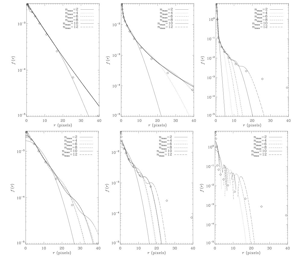 Figure 8
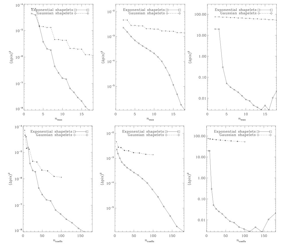 Figure 9
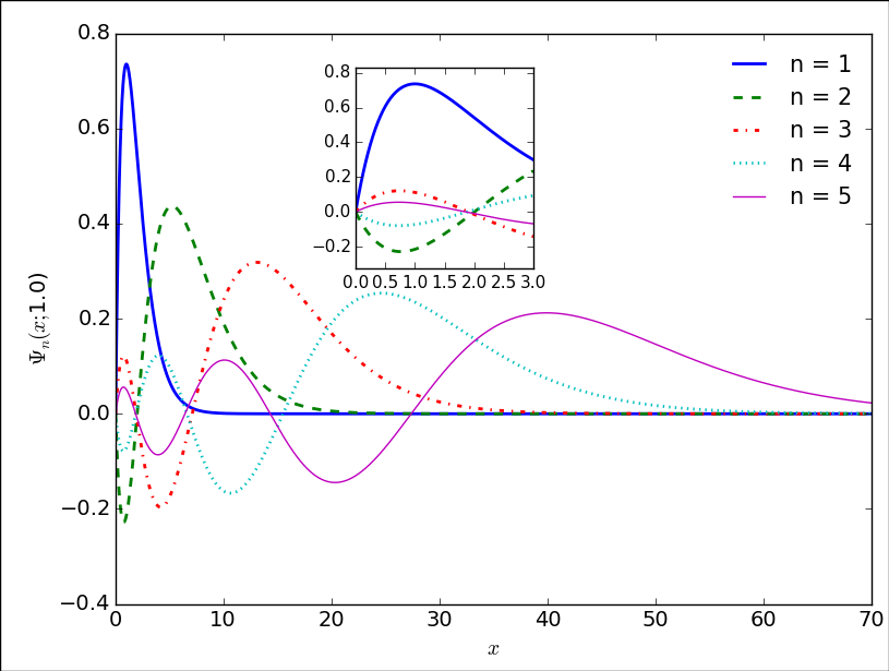 Figure 3
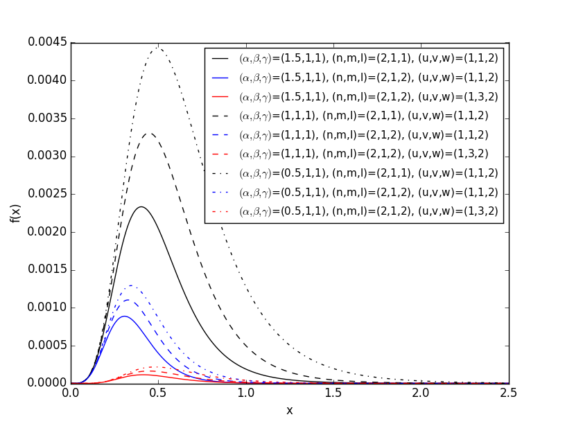 Figure 4
 Figure 5
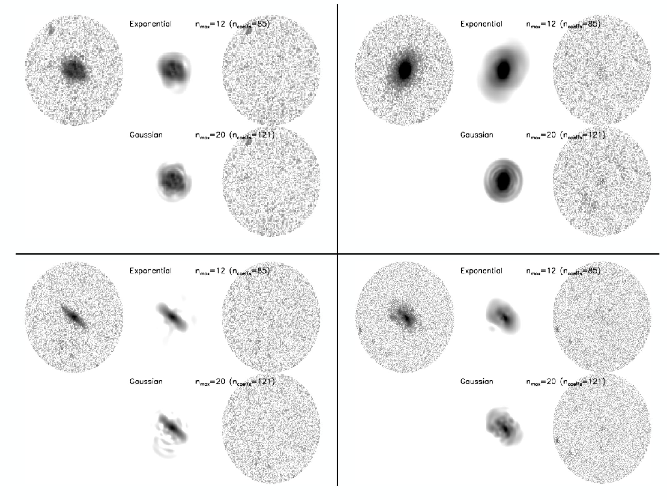 Figure 6
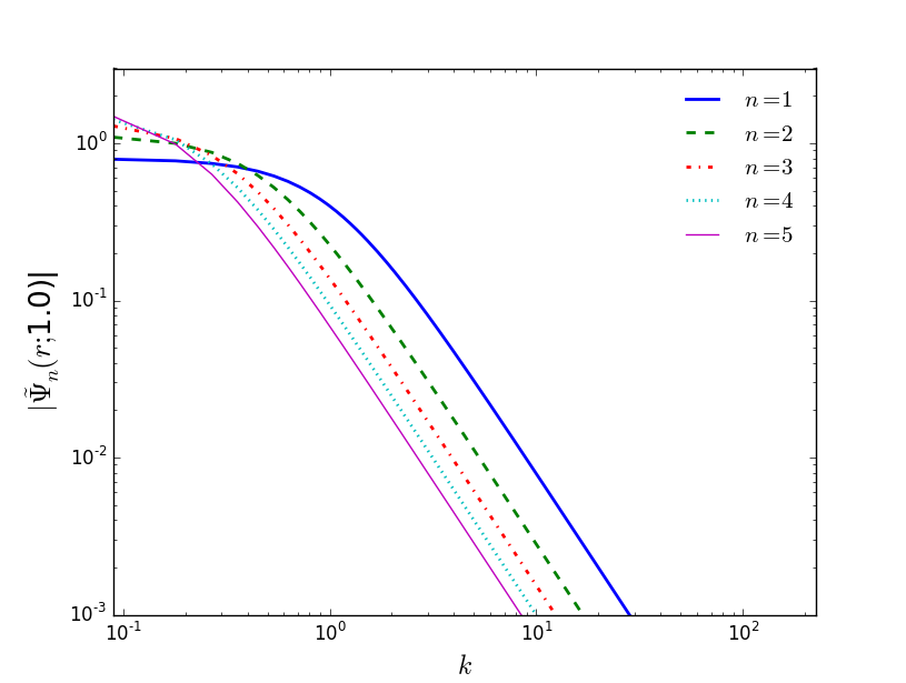 Figure 7
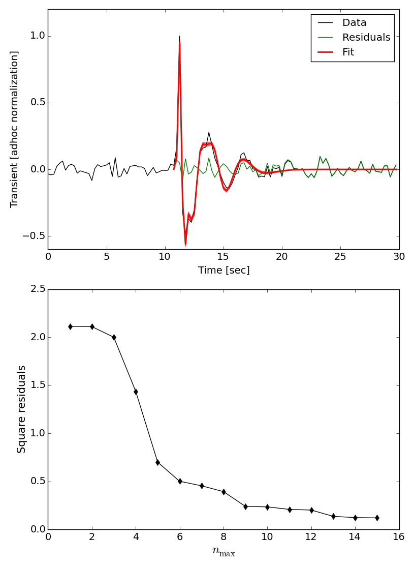 Figure 8
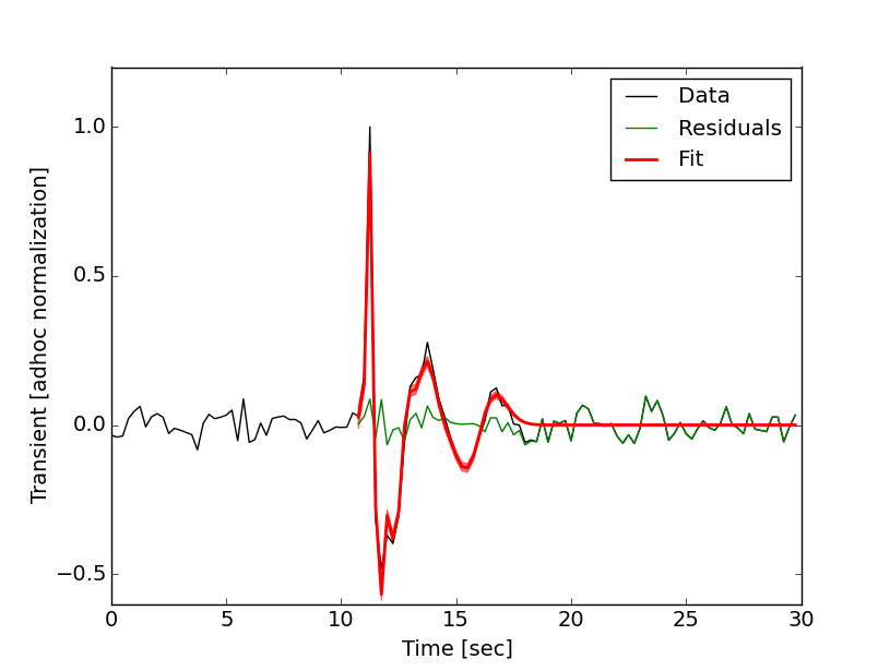 Figure 9
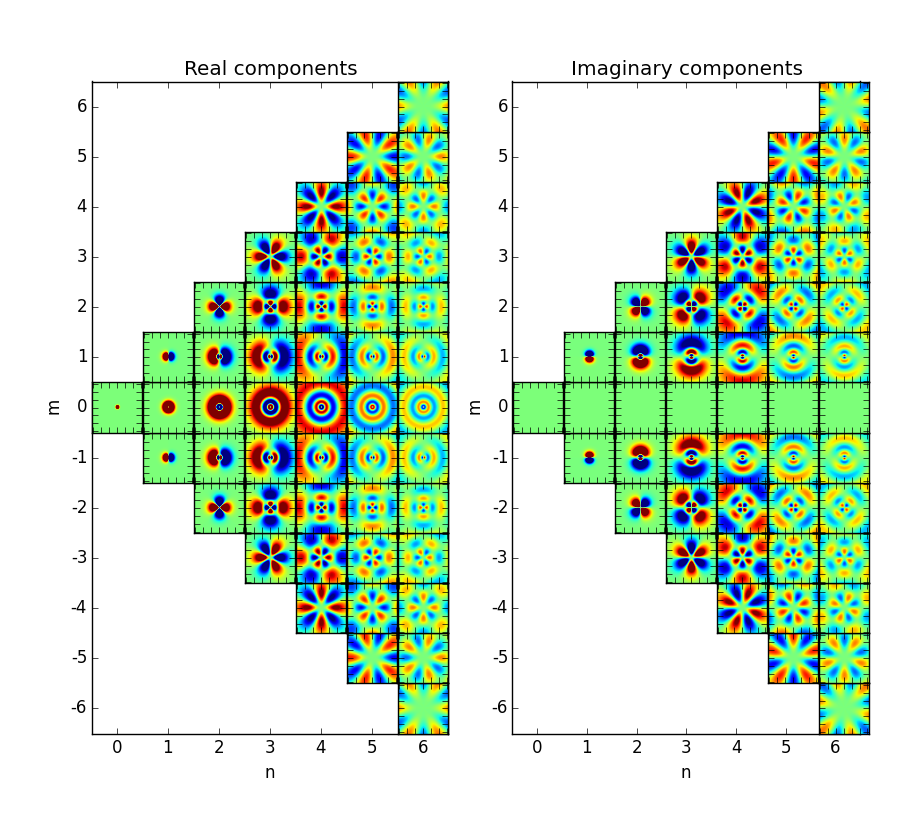 Figure 10
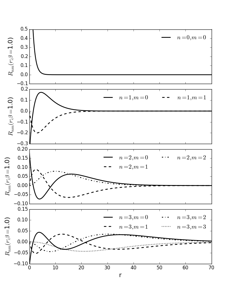 Figure 11
Peer Reviews
No public reviews on file for this paper yet. If you reviewed it on a platform where reviews are public (OpenReview, ICLR, NeurIPS, ICML), you can paste yours below so the community can read it here.
Videos
No videos yet. Explain this paper in a talk, walkthrough, or lecture? Add one.
Exponential shapelets:
basis functions for data analysis of isolated features
Joel Bergé,1 Richard Massey,2 Quentin Baghi,3 and Pierre Touboul4
1DPHY, ONERA, Université Paris Saclay, F-92322 Châtillon, France
2Centre for Extragalactic Astronomy, Department of Physics, Durham University, Durham DH1 3LE, UK
3NASA Goddard Space Flight Center, 8800 Greenbelt Rd, Greenbelt, MD 20771, USA
4DSG, ONERA, Université Paris Saclay, Chemin de la Hunière, F-91123 Palaiseau Cedex, France e-mail: [email protected]
Abstract
We introduce one- and two-dimensional ‘exponential shapelets’: orthonormal basis functions that efficiently model isolated features in data. They are built from eigenfunctions of the quantum mechanical hydrogen atom, and inherit mathematics with elegant properties under Fourier transform, and hence (de)convolution. For a wide variety of data, exponential shapelets compress information better than Gauss-Hermite/Gauss-Laguerre (‘shapelet’) decomposition, and generalise previous attempts that were limited to 1D or circularly symmetric basis functions. We discuss example applications in astronomy, fundamental physics and space geodesy.
keywords:
Methods: Data analysis – Physical data and processes
1 Introduction
A frequent task in data analysis is to categorise and quantify the shapes of localised objects – such as transient events in a (one-dimensional) time-series, or regions of interest in a (two-dimensional) image. It is such a universal challenge that methods developed for one field frequently turn out to be useful in others. For example, astrophysicists measure the shapes of distant galaxies by decomposing them into orthogonal basis functions, such as CHEFs (Jiménez-Teja & Benítez, 2012) or (Gaussian) shapelets (Bernstein & Jarvis 2002; Refregier 2003; Refregier & Bacon 2003; Massey & Refregier 2005). Shapelets have been used to analyse data in other branches of astrophysics, modelling extrasolar planets (Hoekstra et al., 2005; Amara & Quanz, 2012), the distribution of dark matter (Birrer et al., 2015; Tagore & Jackson, 2016), or flashes of pulsars (Lentati et al., 2015; Desvignes et al., 2016; Ellis & Cornish, 2015). They have also been used in medical imaging (Weissman, Hancewicz & Kaplan, 2004; Apostolopoulos et al, 2017), pattern recognition in human vision (Sharpee & Victor, 2009) or artificial vision (Sabzmeydani & Mori, 2007), data compression (Holbrey, 2006), and the manufacture of nanoscale thin films (Suderman et al., 2015; Akdeniz et al., 2018).
Gaussian shapelets are based on eigenfunctions of the quantum mechanics harmonic oscillator. In one-dimensional form, they are Gauss-Hermite functions, which seem to be well adapted in several time-series analyses, especially when transients (whose shape is close to damped oscillations) must be detected, characterised and/or corrected for. This is the case for instance in fundamental physics for MICROSCOPE ‘crackles’ (e.g. Baghi et al. 2015; Bergé et al. 2015), space geodesy for GRACE ‘twangs’ (Flury et al., 2008; Peterseim et al., 2010, 2014) or ‘glitches’ in gravitational waves searches with LIGO (Cornish & Littenberg 2015; Powell et al. 2015, 2017; Principe & Pinto 2017 and references therein). In two-dimensional form, they can be expressed equivalently as either Gauss-Hermite (Cartesian; Refregier 2003) or Gauss-Laguerre (polar; Bernstein & Jarvis 2002; Massey & Refregier 2005) functions. Owing to their quantum mechanical origin, they have elegant properties (they make a complete set) under Fourier transform, and are hence efficient for operations involving convolution or deconvolution of two images.
The main limitation of shapelets is that they are perturbations around a Gaussian, which is flat near its peak. They inefficiently parameterise peaky features, including the distant galaxies for which they were originally suggested (Melchior et al., 2010). Galaxies have a two-dimensional surface density that decreases approximately exponentially with distance from the centre. Capturing the steep gradient near the centre requires a weighted sum of many Gaussian shapelet basis functions, which then overfit noise in the extended wings. Attempting to overcome this limitation, Ngan et al. (2009) developed ‘Sersiclets’, although they were forced to be circularly symmetric, and have not seen wider applications.
In this paper, we extend the quantum mechanical framework underpinning Gaussian shapelets, and define 1D and 2D exponential shapelets based on wavefunctions of the hydrogen atom. These functions are perturbations around a decreasing exponential, and should efficiently model any arbitrarily-shaped but centrally-peaked regions of interest. The perturbations themselves are Laguerre polynomials.
We introduce 1D exponential shapelets in Section 2, and 2D exponential shapelets in Section 3. In both cases, we describe their main properties, compare them to Gaussian shapelets, and provide example uses. We conclude in Section 4.
2 1D exponential shapelets
2.1 Definition
The one-dimensional hydrogen atom is the solution to the motion of a particle in a 1D Coulomb potential . In this paper, we will neither dwell on its rich history, nor the debates about the finitude of its ground state, and about the existence of even wavefunctions (see Nieto 1979; Palma & Raff 2006; Núñez-Yépez et al. 2011, 2014 and references therein). Instead, we simply exploit the normalized 1D hydrogen atom wavefunctions as given by Palma & Raff (2006) to define the 1D exponential shapelet basis functions
[TABLE]
for , where are the generalized Laguerre polynomials (see e.g. Massey & Refregier 2005). The characteristic scale size corresponds to the Bohr radius, and is the eigenfunction energy level.
Note that, contrary to normal procedure in quantum physics, we restrict 1D exponential shapelets on positive , and refrain from defining the negative- part (for ). Hence, we do not follow Palma & Raff (2006) and do not define the even and odd wavefunctions . Events in time series can often be adequately described by their behaviour after a certain moment (in this case, ). Henceforth, we shall therefore drop the + superscript, to write more simply . These functions are continuously differentiable, smoothly departing from zero at and tending back to zero as .
Because the basis functions (1) are eigenfunctions of the one-dimensional hydrogen atom’s Hamiltonian, they form an orthogonal basis of the square integrable functions Hilbert space equiped with the inner product and an asterisk denotes complex conjugation. They are orthonormal, in the sense that where is the Kronecker symbol, and complete, in the sense that .
They thus form a basis, on which we can uniquely decompose a function as
[TABLE]
with coefficients given by an overlap integral
[TABLE]
Bessel’s inequality then assures us that for any function ,
[TABLE]
where is the L2 norm, so that the series (2) converges and coefficients must vanish as increases. The series can therefore be truncated for suitably localised functions, at some value .
2.2 Properties
2.2.1 Maximum and minimum effective scales
The first few 1D exponential shapelet basis functions are shown in Fig. 1. As the order increases (with constant ), the largest-scale oscillation dominates, and rapidly acquires a larger extent. However, the smallest oscillations always remain roughly the same size.
To act as a convenient figure-of-merit, we follow Refregier (2003) in defining the largest scale that can be described by an exponential shapelet model as
[TABLE]
Empirically, the smallest scale that can be described is
[TABLE]
As , the range of scales modelled by a 1D exponential shapelet decomposition, . However, the resolution of an exponential shapelet model is greatest near the origin, and decreases away from it. This behaviour is very different from Gaussian shapelets, where the resolution is more spatially uniform: increasing increases the scale of the model slowly, while simultaneously adding smaller-scale oscillations (see Fig. 1 of Refregier 2003). The wide effective range of scales for exponential shapelets is what will allow them to efficiently describe spiky but long-duration events.
2.2.2 Fourier and Laplace transforms
To compute the Fourier transform of the 1D exponential shapelet basis functions, we adopt a convention where the Fourier transform is defined as
[TABLE]
for any function , where . The Fourier transform of the basis function is then (setting for )
[TABLE]
Note that the real part of the Fourier transform is even for all , while its imaginary part is odd for all . Its modulus is a Lorentzian function centered on whose width parameter is inversely proportional to (as typical for exponentially suppressed oscillations)
[TABLE]
With conventions similar to those for the Fourier transform, the Laplace transform is given by
[TABLE]
Although Eqs. (8) and (10) are not as simple as for Gaussian shapelets (the Fourier transform of a Gaussian shapelet is itself a Gaussian shapelet), closed forms exist for exponential shapelets that are easy to implement. The Fourier and Laplace transforms of 1D exponential shapelets are also well localized in frequency space (Fig. 2).
2.2.3 Convolution
Convolution is an inevitable operation during signal acquisition, whereby an input (‘real’) signal undergoes the measurement apparatus’ transfer function. What is ultimately measured is the convolution of the input signal with the transfer function.
Let us consider the convolution of two functions and , whose convolution product is
[TABLE]
Following the same arguments as Refregier (2003), the functions can all be decomposed into exponential shapelets, perhaps with different scale sizes , and . We can then relate the 1D exponential shapelet space coefficients to and via
[TABLE]
where the convolution tensor is given by
[TABLE]
and is the binomial coefficient. A proof of Eq. (13) is provided in Appendix A.1.
The integral
[TABLE]
appearing in Eq. (13) is zero if is odd (a proof is provided in Appendix A.2). Hence, is always wholly real. Under some conditions, it can be estimated analytically and expressed as a sum of converging series (see Eqs. 59, 63 and 70 in Appendix A.3). Those conditions are often not met, but the integrand is a well-behaved function, so the integration can also be performed numerically. We find that numerical integration is most convenient if the function is cut into three segments (see Eqs. 55, 61 and 68 in Appendix A.3).
2.2.4 Rescaling
1D exponential shapelets obey the integral property
[TABLE]
Using this, it can be shown that under a rescaling , the coefficients of a model (3) transform as
[TABLE]
and under , the coefficients are themselves multiplied by .
2.3 Shape characterization
Let be a 1D object decomposed into 1D exponential shapelets. In terms of its shapelet coefficients, its integral (total ‘flux’) is
[TABLE]
which can be readily shown from the integral property (15).
Provided , its barycenter (centroid) is
[TABLE]
and it has a characteristic size
[TABLE]
This size can be used to determine the exponential decay rate of the object, for instance, when modelling damped oscillations.
Note that series (19) converges only if the amplitudes of the 1D exponential shapelet coefficients decrease faster than , which may not always be the case. Care must therefore be taken to check for convergence when characterising the shape of a feature using this technique.
2.4 Exponential shapelets modelling in practice
As shown above (Eq. 2), a 1D feature is straightforward to model for a given couple (, ), where is the maximum order of the truncated sum (2). For example, a linear least-square method can be efficiently used for this purpose. Then the model depends non-linearly on the two parameters and that can be optimised by iteratively minimizing the residuals between the observed feature and its model. This procedure was described at length, in the 2D case, by Massey & Refregier (2005).
2.5 Example applications
This section demonstrates three possible applications of 1D exponential shapelets. We start by modelling exponentially suppressed oscillations, which are measurements throughout experimental physics, including the response of accelerometers111http://www.onera.fr/en/dphy onboard the space missions MICROSCOPE (Touboul et al., 2017), GRACE (Tapley et al., 2004) and GOCE (Rummel et al., 2011). We then discuss a potential application to unmodelled bursts in the analysis of gravitational waves. Exponential shapelets may also be convenient to model charge transfer inefficiency trailing due to radiation damage in spacebourne imaging detectors (Massey et al., 2010), although we do not explore that further here.
2.5.1 Cleaning accelerometer time series data, and modelling an experiment’s response function
MICROSCOPE tested the Weak Equivalence Principle (WEP) by precisely measuring the differential acceleration experienced by two concentric cylindrical test-masses onboard a drag-free satellite in Low Earth Orbit222The mission ended on October 16, 2018; data analysis is still underway.. In theory, any non-zero difference at a well defined frequency (which depends on the orbit and attitude characteristics of the satellite) is a signature of the violation of the WEP.
In practice, many transients are apparent in MICROSCOPE data (the upper panel of Fig. 3 shows a typical high-signal-to-noise example). These transients are generally caused by crackles of the satellite’s coating (because of temperature variations), crackles of the satellite’s gas tanks (as their pressure decreases as the gas is consumed), or impacts with micro-meteorites. Such transients occupy frequencies higher than , so they do not directly impact a possible WEP violation signal. However, it is necessary to detect and mask them in measured time-series, then either reconstruct the corresponding ‘missing data’ (Bergé et al., 2015; Pires et al., 2016) to allow for a least square fit of the expected WEP violation signal in the frequency domain (Touboul et al., 2017), or adapt the maximum likelihood technique to take missing data into account (Baghi et al., 2015, 2016). Existing techniques are suboptimal, as they may affect the noise characteristics. Moreover, transients could be considered as conveying useful information. They are created by an external impulse; if this is assumed to be instantaneous (Dirac), the shape and relaxation time of the observed signal is a measurement of MICROSCOPE’s transfer function.
1D exponential shapelets are well-matched to these transient signals. The upper panel of Fig. 3 shows a transient in the time domain: the observed data are shown in black, a model (fitted between s and s) and its 68% confidence interval are shown in red, and residuals consistent with noise are shown in green. This model uses , meaning that it has compressed 60 data points in the time domain description (15 seconds sampled at 4Hz) into 15 shapelet coefficients. Nonetheless, the model has rich, empirical freedom to capture multiple response modes of the instrument’s complex structure. The lower panel of Fig. 3 shows the convergence of the model as we increase , quantified as the square residuals between the observed transient and the model. Most of the information is contained in coefficients .
An extension to this process will be presented in a future paper. By fitting 1D exponential shapelet coefficients to many transients, it is possible to model temporal variations in MICROSCOPE’s instrument’s relaxation time via parameter or the exponential envelope scale . Interpolating these models then yields a model of the transfer function at any time, to either gain insight into the instrument’s performance, or to correct (deconvolve) signals with an ‘inverse transfer function’ transform. Note that this procedure is similar to techniques developed for 2D astronomical image processing, where a Point Spread Function (PSF) is determined from the shape of stars then interpolated across the data (see e.g. Bergé et al. 2012; Gentile et al. 2013; Kilbinger 2015).
2.5.2 Characterisation of perturbing signals in space-borne geodesy missions
The GRACE mission (Tapley et al., 2004) revolutionised geodesy by measuring the Earth’s gravitational field with unprecedented precision. Two satellites followed each other on the same orbit, monitoring the distance between them via microwave ranging. In theory, any variation in their relative speed or distance can be ascribed to variations in the Earth’s geopotential.
In practice, the satellites were also subject to non-gravitational forces. These were measured by ultrasensitive accelerometers, for removal during post-processing (Flury et al., 2008; Peterseim et al., 2010). Peterseim (2014) and Peterseim et al. (2014) modelled transients (known as ‘spikes’) in accelerometer data using a piecewise function made from the derivative of a Gaussian, a 3rd order polynomial and a damped oscillation. Some were successfully classified as due to either the satellite’s heaters, or activation of its magnetic torquers – but no physical origin could be assigned to others, known as ‘twangs’.
Tentative correlations of twangs with the position of the satellite along its orbit hint at a possible geophysical origin. Both categories of twangs are compactly-represented as 1D exponential shapelets, so we will investigate in a future paper whether these provide a cleaner set of shape parameters to categorise and understand their origin.
2.5.3 Unmodelled bursts and glitches in gravitational waves data analysis
A wealth of methods have been developed to search for, characterise and classify unmodelled bursts and instrumental glitches in searches for gravitational waves (see e.g. Cornish & Littenberg, 2015; Powell et al., 2015, 2017; Principe & Pinto, 2017, and references therein). Glitches are often modelled using ‘Sine-Gaussian waveforms’ (Principe & Pinto, 2017). These have similar properties to Gaussian shapelets, although shapelets can encode more details. 1D exponential shapelets could further optimise the data compression of complex glitch shapes that often exhibit damped oscillations.
Shapelets might therefore improve the detection, characterisation and classification of instrumental glitches in gravitational wave detectors. Indeed, bursts and glitches are usually detected in the time-frequency domain, which is easily reproduced in Gaussian shapelets-time space. If 1D exponential shapelets more efficiently model the information in a glitch, exponential shapelet-time space would be even better. We will investigate in a future paper whether glitches can be detected by scanning a matched-filter, and correlating the measured signal with a 1D exponential shapelet model, while leaving (and possibly ) free.
2.6 Comparison with Gaussian shapelets
The MICROSCOPE transient modelled as exponential shapelets () in Fig. 3, is modelled as Gaussian shapelets () in Fig. 4. Achieving a similar precision of fit requires more coefficients, and creates more small-scale artefacts: the data are over-fit near the centre of the model, and underfit at the extremes. We also find that its coefficients are highly covariant, with the good fit produced by large positive and negative basis functions almost precisely cancelling each other. This is much less apparent for the 1D exponential shapelet coefficients. Indeed, we find that estimating the model again on points different from those observed data fails to reproduce the overall shape of the transient, whereas the 1D exponential shapelet model is itself predictive.
In this example, it appears that 1D exponential shapelets outperform Gaussian shapelets. This is because their perturbations around an exponential decay are better matched to the underlying signal, and because their wider extent spreads information density more evenly. In general, the type of shapelet to choose should depend on the decay rate of the target function.
3 2D exponential shapelets
3.1 Definition
The quantum mechanics of a hydrogen atom restricted to two dimensions is well studied (see e.g. Zaslow & Zandler, 1967; Yang et al., 1991; Chaos-Cador & Ley-Koo, 2007). The bound states of the electron (i.e. eigenfunctions of the Hamiltonian) provide a natural set of basis functions to represent a bounded distribution. After renormalizing these, we define the 2D exponential shapelet basis functions
[TABLE]
for , where are generalized Laguerre polynomials. The term is used to ensure that the integral of each basis function is positive, but this is otherwise the form used in quantum theory. In terms of quantum mechanics, is the principal quantum number (the eigenfunction energy level) and the magnetic quantum number, which takes integer values between and . The characteristic scale is linked to the Bohr radius.
These functions form an orthonormal set of basis functions in the space equipped with inner product .
Any localized function can be uniquely decomposed into a weighted sum of these basis functions
[TABLE]
where the 2D exponential shapelet coefficients are given by
[TABLE]
Using Bessel’s inequality like in the 1D case, we find that series (21) converges, and the coefficients must vanish when and increase. For a real function , . In this case, truncating the series at results in independent coefficients.
It may also be possible to define elliptical 2D exponential shapelets by applying a shear transformation to the coordinate system, as Nakajima & Bernstein (2007) suggested for Gaussian shapelets. This preserves their orthonormality, and can increase their rate of data compression, at the cost of two additional non-linear parameters to specify the shear.
3.2 Properties
3.2.1 Maximum and minimum effective scales
The first few 2D exponential shapelet basis functions are illustrated in Fig. 5, and their radial component is shown in Fig. 6, defined via . Their resemblance with Gaussian polar shapelets is striking (see Fig. 2 of Massey & Refregier, 2005). However, due to their exponential kernel, exponential shapelets are both more peaky and further spread out than Gaussian shapelets. The size difference between the lowest order basis function and even a low order one like is striking. It is this behaviour that will help to describe spatially extended features.
Generalising the 1D case (Section 2.2.1), we define the largest effective scale in a 2D exponential shapelet model as
[TABLE]
Again empirically, the smallest resolved scales are roughly constant,
[TABLE]
The range of scales included in a 2D exponential shapelet model as is . The resolution of an exponential shapelet model is greatest near the origin, and information density is concentrated there. This behaviour is different from the Gaussian shapelets, where resolution is more spatially uniform, and information density is constant, with .
3.2.2 Fourier transformation and convolution
Using the same convention as in the 1D case, it can be shown that the Fourier transform of 2D exponential shapelets is given by
[TABLE]
where , is the angle between the direction and the direction in polar space, and is the Hankel transform of the radial function. Consequently, the convolution tensor involved in the convolution of two objects modelled in 2D exponential shapelets is the integral of products of Hankel transforms of functions. We were not able to find an analytic form for this Hankel transform, so it must instead be computed numerically.
3.2.3 Coordinate transforms
It can be useful to know the response of the basis functions to 2D linear coordinate transforms: either to know how to mix the coefficients of a shapelet decomposition in order to perform that transform, or to form combinations of coefficients that are invariant under some transforms. This was used to construct estimators of the shear distortion applied to images of galaxies by the effect of weak gravitational lensing (Kuijken, 2006; Massey et al., 2007).
A convenient shortcut to calculating those transforms for Gaussian shapelets was provided by the ladder operators associated with the quantum mechanical harmonic oscillator (Refregier & Bacon, 2003). Unfortunately, we have not yet found a useful form of the ladder operators for the 2D hydrogen atom. If it becomes necessary to perform linear transformations on 2D exponential shapelets, it will be necessary to apply the transforms manually to the basis functions (a long and arduous task, but one that is guaranteed to yield a closed form, because the basis is complete).
3.3 Object shape measurement
Once a feature has been decomposed into 2D exponential shapelets, its coefficients can be used to construct characteristic measurements of its shape. In this section, we derive expressions for an object’s (azimuthally-averaged) radial profile, flux, centroid, unweighted quadrupoles, size and ellipticity, in terms of its shapelet coefficients. We have not attempted it here, but it should also be possible to develop an exponential-shapelet classification of galaxy morphologies via e.g. their concentration, asymmetry and symmetry (Conselice et al., 2000).
3.3.1 Radial profile
Azimuthally averaging an object’s signal yields its mean radial profile
[TABLE]
Noting that all basis functions average to zero, the radial profile reduces to
[TABLE]
where the (rotationally invariant) basis functions are
[TABLE]
Eq. (27) is identical to the equivalent derivation for Gaussian shapelets (see Eq. (16) of Massey & Refregier, 2005), up to the fact that basis functions with odd do not exist in the Gaussian case.
3.3.2 Flux
Integrating the signal inside a circular aperture of radius yields its ‘flux’
[TABLE]
To evaluate this integral, it is useful to note that, once again, all basis functions cancel out to zero during integration over , and also a closed form for the generalized Laguerre polynomials,
[TABLE]
Using this, it can be shown that
[TABLE]
where is the lower incomplete gamma function. Extrapolating to large radius, and taking the limit , we obtain
[TABLE]
3.3.3 Centroid
Similarly, it can be shown that the unweighted centroid (), defined by
[TABLE]
is, in terms of 2D exponential shapelet coefficients,
[TABLE]
3.3.4 Quadrupole moments
The unweighted quadrupole moments of an object
[TABLE]
can be used to define quantities such as its rms size and ellipticity (see below). They are, in terms of 2D exponential shapelet coefficients,
[TABLE]
[TABLE]
[TABLE]
3.3.5 Size and ellipticity
Using Eqs. (36)-(38), expressions can be obtained to quantify a feature’s size
[TABLE]
and ellipticity
[TABLE]
In this complex notation with , denotes rotational invariance, and a positive real (imaginary) component denotes elongation along (at to) the -axis.
3.3.6 Convergence
Expressions for the shape estimators resemble those obtained for polar Gaussian shapelets in Section 6 of Massey & Refregier (2005). In particular, a feature’s radial profile, flux and size are encoded within the coefficients, while the centroid is described by the coefficients and ellipticity by the coefficients. The expressions also contain the same power of as those for Gaussian shapelets, because that encodes information about the units in which the data is expressed.
However, shape measures for 2D exponential shapelets contain higher powers of than those for 2D Gaussian shapelets, and will converge more slowly. Some of this is due to the normalisation of the basis functions against an inner product. In the Gaussian shapelet case, this happens to yield an integral of basis functions (32) that is independent of , while in exponential shapelets it is . That power of could have been included in the basis functions and removed from the coefficients – although doing so would merely make them look more stable rather than actually altering convergence. In the limit that , convergence of the flux estimator requires to decrease faster than ; convergence of centroid requires to decrease faster than ; convergence of size and ellipticity requires and to decrease faster than . This may not be a problem, since we expect 2D exponential shapelets to converge faster than shapelets (i.e. to have a lower for a given galaxy). However, if this does not hold true, for example due to measurement noise, care should be taken to restrict the decomposition and measurement of photometry inside a finite aperture, or to truncate the 2D exponential shapelet model at finite .
3.4 Example application
This section demonstrates the use of 2D exponential shapelets to model the shapes of galaxies seen outside our own Milky Way (they may also be convenient to model the shapes of gamma-ray events; S. Pires, private communication). We examine the convergence speed of 2D exponential shapelets, and compare their performance to that of 2D Gaussian shapelets.
3.4.1 Distant galaxies in astronomical imaging
Galaxies are collections of (hundreds of billions of) stars, with a combined surface brightness that peaks sharply near the centre, and decreases to large radii in a way that is often exponential. Four galaxies in the COSMOS survey (Scoville et al., 2007a, b) observed by the Hubble Space Telescope (Koekemoer et al., 2007), are shown in Fig. 7. As mentioned in Sect. 2.4 for the 1D case, we follow the algorithm described by Massey & Refregier (2005) to choose the best non-linear parameters of the models –, and centroid). Note that galaxies in this figure were modelled into shapelets with the “diamond” truncation scheme introduced in Massey et al. (2007), which is intended to reduce small scales oscillations by ignoring the higher terms of the decomposition. In this case, the number of coefficients is divided by 2, allowing also a better compression of the information.
In all four cases, 2D exponential shapelets require fewer coefficients (lower ; here ) to provide a model whose residuals are consistent with the noise than Gaussian shapelets (here ). Even more interestingly, exponential shapelets tend to provide a (visually) cleaner model of the central region of the galaxies. The top left galaxy has an irregular morphology, and the 2D exponential shapelet model shows fewer artifacts than the polar shapelet model. For an elliptical (top right) or edge-on spiral galaxy (bottom left), the ringing common in Gaussian shapelets disappears with 2D exponential shapelets: they do not possess high-frequency ripples at large radii that need large coefficients alternating in sign for them to cancel. Even for highly eccentric galaxies (bottom right), 2D exponential shapelets provide cleaner models than polar shapelets, especially in the outskirts of the galaxies, as the exponential wings are fundamentally a better match to the underlying signal.
3.4.2 Convergence speed
To assess the ability of 2D exponential shapelets to model galaxies, we require noise-free images whose true properties are known. We simulate elliptical galaxies with a Sersic radial profile
[TABLE]
where is the galaxy’s s profile, is the Sersic index, is a normalisation constant and is the effective radius (which contains 50% of the galaxy’s flux). We simulate three types of galaxies: exponential (), intermediate (), and de Vaucouleurs ().
Fig. 8 compares the radial profiles fitted with 2D exponential shapelets (upper row) or Gaussian shapelets (lower row), for different maximum orders of decomposition , and coarsely optimised (this could be further optimised at low in the presence of noise). The normalisation of the ordinate depends on and pixellisation, so is arbitrary; only its relative scaling is informative. For all three galaxy types, 2D exponential shapelets greatly outperform Gaussian shapelets. A decomposition to or is sufficient to model an exponential galaxy. Depending on the signal-to-noise of real data, a decomposition to may be sufficient for an intermediate galaxy. It is more challenging to model a de Vaucouleurs galaxy, and even exponential shapelets require to capture its extended tails three orders of magnitude fainter than the peak. However, they do so without the oscillatory ‘ringing’ introduced by the cancellation of positive and negative basis functions in Gaussian shapelets.
To illustrate the convergence speed, Fig. 9 shows the mean square residual of the models of the same galaxies as in Fig. 8, as a function of the maximum shapelet order (upper row), or the total number of coefficients . The normalisation of the ordinate is arbitrary, and only its relative scaling is informative. Once again, it is clear that 2D exponential shapelets (solid lines) outperform Gaussian shapelets (dashed lines). For exponential and intermediate galaxies (left and middle columns), the residual of the 2D exponential shapelet model decreases consistently, and ends up several orders of magnitude better than that of Gaussian shapelets. The enhanced performance of exponential shapelets is even more prominent for a de Vaucouleurs galaxy. The limitation for exponential shapelets in this case is numerical precision of our algorithm to pixellate the basis functions. At high-, this breaks down, causing spurious residuals at the very centre of the model, shown as an artificial upturn in the bottom-right panel of Fig. 9. This could be circumvented by more accurate pixellisation, or by imposing limits on .
4 Conclusion
In this paper, we introduced exponential shapelets, a family of orthonormal basis functions that can be efficiently used to model 1D and 2D objects. They borrow many concepts from the original Gaussian shapelets, but are perturbations around a decaying exponential rather than a Gaussian, and more efficiently compress the information in damped 1D oscillations or centrally-concentrated 2D features. In particular, they can simultaneously capture the central peak and the extended wings of galaxies in astronomical imaging, thereby solving the main criticism levelled at Gaussian shapelets in the field for which they were originally intended.
Modelling a feature using exponential shapelets first requires a choice of characteristic scale size and expansion order ; these can be selected using an non-linear optimisation method developed for Gaussian shapelets (Massey & Refregier, 2005). The function is then decomposed into a weighted sum of exponential shapelet basis functions using linear regression. A least-squares fit is often sufficient, although in some cases, modeling a transient may be stabilised by regularisation techniques such as sparsity constraints.
Once a feature is described as a weighted sum of exponential shapelets, simple combinations of the weights yield expressions for its total flux, centroid, size and ellipticity. These are similar to those for Gaussian shapelets. However, convolution and deconvolution in exponential shapelets is significantly more difficult than the Gaussian case, with the convolution tensor being time-consuming to calculate via numerical integration.
We described possible applications of exponential shapelets in several fields of experimental and observational science. 1D exponential shapelets can be used to model (and subtract or understand) spurious transients in time series, such as measurements by the MICROSCOPE or GRACE satellites, or the LIGO search for gravitational waves. Thanks to their exponential decay, 2D exponential shapelets overcome the main criticism aimed at Gaussian shapelets (though at the cost of losing some simplicity) and can be used to measure the brightness, shape and size of distant galaxies in astronomical imaging. The characteristics of exponential shapelets should make them well-suited to data compression and analysis in a wide range of fields; their convenient mathematical properties should see them frequently adopted.
Acknowledgments
The concepts in this paper matured over many years, after a preliminary study to generalise Gaussian polar shapelets for Hubble Space Telescope data, for which we acknowledge support from NASA through grant HST-AR-11747 – and which was carried out at the Jet Propulsion Laboratory, California Institute of Technology, under a contract with NASA. We are indebted to Barnaby Rowe for researching Kummer functions and the literature of the 2D hydrogen atom. We also acknowledge helpful and motivating discussions with Jason Rhodes, Richard Ellis, Alexandre Refregier, Sandrine Pires, James Nightingale, Bernard Foulon, Bruno Christophe, Gilles Métris, Manuel Rodrigues, Alain Robert and Nicolas Touquoy. This work makes use of technical data from the CNES-ESA-ONERA-CNRS-OCA Microscope mission, and has received financial support from ONERA and CNES. JB acknowledges the financial support of the UnivEarthS Labex program at Sorbonne Paris Cité (ANR-10-LABX-0023 and ANR-11-IDEX-0005-02) and of CNES through the APR programme (LISA project). RM is supported by a Royal Society University Research Fellowship and through STFC grant ST/N001494/1.
Appendix A Derivation of convolution kernel tensor for 1D exponential shapelets
A.1 Proof of Eq. (13)
Let and two 1-dimensional functions, whose convolution product is . In Fourier space, , where
[TABLE]
and similarly for .
Decomposing and into exponential shapelets (), substituting in Eq. (42) and re-arranging terms, we get
[TABLE]
where we recall that
[TABLE]
Using the Parseval-Plancherel theorem, we get
[TABLE]
where the bar denotes the complex conjugate.
Substituting Eq. (43) in Eq. (45), and re-arranging terms, we find
[TABLE]
which defines such that
[TABLE]
The final expression for (Eq. 13) is then found using the binomial decompositions of , and .
It can noted that is a complex number, unless is even, such that . If is odd, then the integral is 0 (see A.2). Hence, we do not need to impose any restriction on for to be real. We can also note that since , and , the integral in Eq. (13) converges.
We will then aim to look for an analytic expression for the integral in Eq. (13). We introduce
[TABLE]
A.2 Properties of ’s integrand
In this section, we derive some properties of the integrand that appears in the definition of . Let us name it (rigorously, we should write , but we drop the indices to simplify the notation), such that
[TABLE]
where , and (see Eq. 13).
A.2.1 Alternative definition
When developping binomial expressions in , we get another form for the function, that appears as the inverse of a series of
[TABLE]
A.2.2 Parity
It is obvious that , so that is even (resp. odd) when is even (resp. odd). Hence, vanishes when is odd, in which case . As mentioned in the main text, is real if is even (then, is real for all combinations of , , , , , ). In the remainder of this appendix, we restrict ourselves to .
A.2.3 Value in 0
Evidently, if . If , then .
A.2.4 Limit at
Since , and , it is easy to see that .
A.2.5 Dependence on , ,
For a given , quickly decreases as (and similarly for and ), showing that only the contributions of low , and are significant in . Then, the series (Eq. 47) converges quickly.
The left panel of Fig. 10 shows for some realistic combinations . It can be seen that is well-behaved, and tends quickly towards 0 for large . Its extend depends on , and . As mentioned above, for a given , it quickly decreases when , , increase. The right panel of Fig. 10 shows when , = 2, = 1 = 1, = 2, and , together with the values and (borders of the grey area), which are key values in computing (see below).
A.3 Computation of the integral in
We now turn to look for an analytic expression for . We first note that, due to the parity property of ,
[TABLE]
if is even, or otherwise.
We decompose as
[TABLE]
where, as we show below, we impose and .
A.3.1 Computation of first integral in r.h.s. of Eq. (52)
We first introduce
[TABLE]
where, for clarity, we wrote with all its indices.
Changing variable such that , we get
[TABLE]
Another change of variable, , gives
[TABLE]
where we can recognize, if , Lauricella’s function of the fourth kind (e.g. Bezrodnykh 2016; Hasanov & Srivastava 2007)
[TABLE]
with , , , , , , , and , such that
[TABLE]
is defined (as long as ) as a converging series (Eq. (1.4) in Hasanov & Srivastava 2007), such that
[TABLE]
where is the Pochhammer symbol, such that (after simplifying Pochhammer symbols):
[TABLE]
A.3.2 Computation of second integral in r.h.s. of Eq. (52)
We then introduce
[TABLE]
that we will compute in a similar fashion as the previous integral.
With successive changes of variables , , and (under our assumptions, ; if , ), we obtain
[TABLE]
If , then must be calculated numerically. This is the case in the example of Fig. 10. However, if (i.e. , then we recognize a Lauricella function, such that
[TABLE]
If , can finally be expressed as a converging series
[TABLE]
A.3.3 Computation of third integral in r.h.s of Eq. (52)
We now introduce
[TABLE]
that we will compute in a similar fashion as and .
We first note that , where for simplicity, we droped the indices from the definition, and is some positive cut-off, and
[TABLE]
can be computed using successive changes of variable. First, we set , so that (after rearranging some terms)
[TABLE]
Additional changes of variables (, , ) then yield
[TABLE]
where . Taking the limit , we obtain
[TABLE]
Under the assumption that , we recognize a Lauricella function, such that
[TABLE]
and we can finally express as a converging series
[TABLE]
The reference list from the paper itself. Each links out to its DOI / PubMed record.
- 1Amara & Quanz (2012) Amara, A. & Quanz S., 2012, MNRAS, 427, 948
- 2Apostolopoulos et al. (2014) Apostolopoulos, G., Koutras, A., Christoyianni, I. and Dermatas, E., 2014, May. Computer aided classification of mammographic tissue using shapelets and support vector machines. In Hellenic Conference on Artificial Intelligence (pp. 510-520). Springer, Cham.
- 3Apostolopoulos et al (2017) Apostolopoulos, G., Koutras, A., Christoyianni, I., & Dermatas, E., 2017, IEEE 25th European Signal Processing Conference (EUSIPCO) 56-60
- 4Baghi et al. (2015) Baghi, Q., Métris, G., Bergé, J., et al. 2015, Phys. Rev. D, 91, 062003
- 5Baghi et al. (2016) Baghi, Q., Métris, G., Bergé, J., et al. 2016, Phys. Rev. D, 93, 122007
- 6Bergé et al. (2015) Bergé, J., Pires, S., Baghi, Q., Touboul, P., & Métris, G. 2015, Phys. Rev. D, 92, 112006
- 7Bergé et al. (2012) Bergé, J., Price, S., Amara, A., & Rhodes, J. 2012, MNRAS, 419, 2356
- 8Bezrodnykh (2016) Bezrodnykh, S.I. 2016, Mathematical notes, Vol. 100, No. 2, pp. 318