FAVE: A fast and efficient network Flow AVailability Estimation method with bounded relative error
Tingwei Liu, John C.S. Lui

TL;DR
FAVE is a novel, fast, and efficient method for estimating network flow availability with bounded error, significantly reducing computational costs compared to traditional Monte Carlo and importance sampling techniques.
Contribution
The paper introduces FAVE, a new sequential importance sampling approach that achieves bounded or vanishing relative error with linear complexity for flow availability estimation.
Findings
Reduces estimation cost by up to 900 times compared to Monte Carlo.
Achieves bounded or vanishing relative error with linear complexity.
Improves capacity planning accuracy with better flow availability guarantees.
Abstract
This paper focuses on helping network providers to carry out network capacity planning and sales projection by answering the question: For a given topology and capacity, whether the network can serve current flow demands with high probabilities? We name such probability as "{\it flow availability}", and present the \underline{f}low \underline{av}ailability \underline{e}stimation (FAVE) problem, which is a generalisation of network connectivity or maximum flow reliability estimations. Realistic networks are often large and dynamic, so flow availabilities cannot be evaluated analytically and simulation is often used. However, naive Monte Carlo (MC) or importance sampling (IS) techniques take an excessive amount of time. To quickly estimate flow availabilities, we utilize the correlations among link and flow failures to figure out the importance of roles played by different links in flow…
Click any figure to enlarge with its caption.
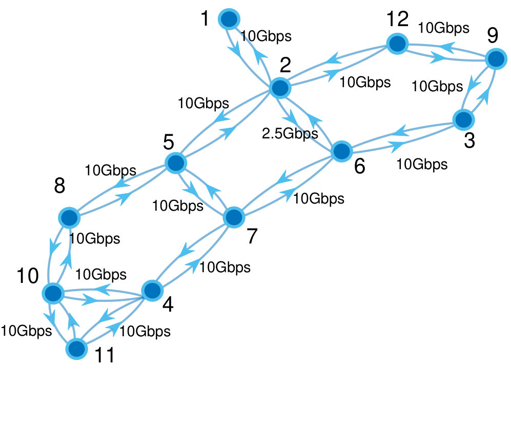 Figure 1
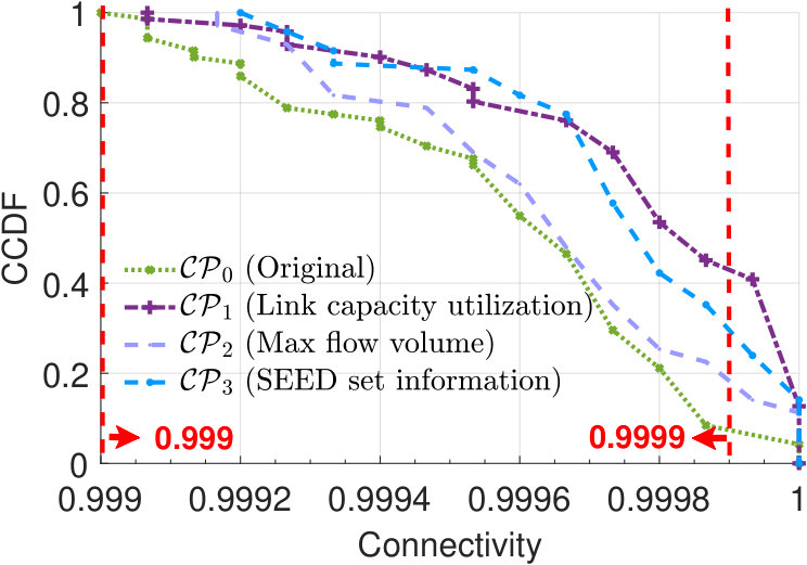 Figure 2
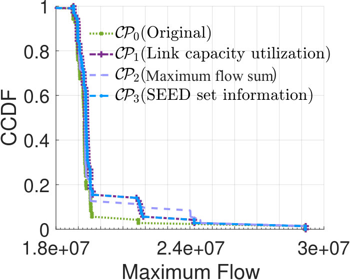 Figure 3
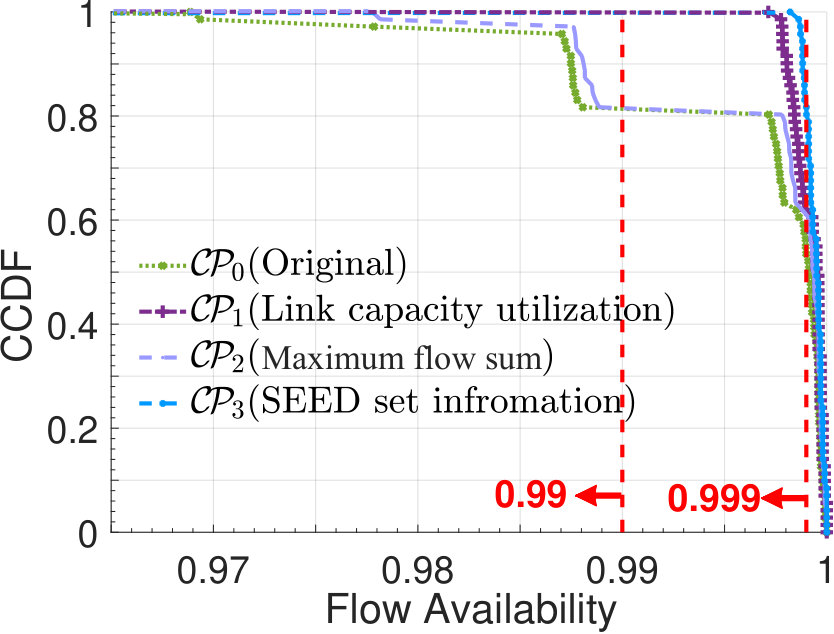 Figure 4
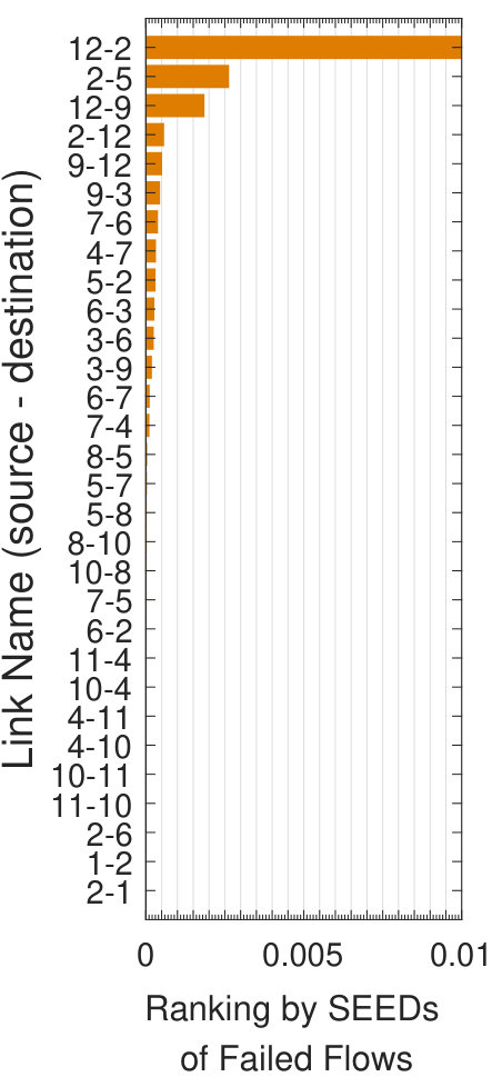 Figure 5
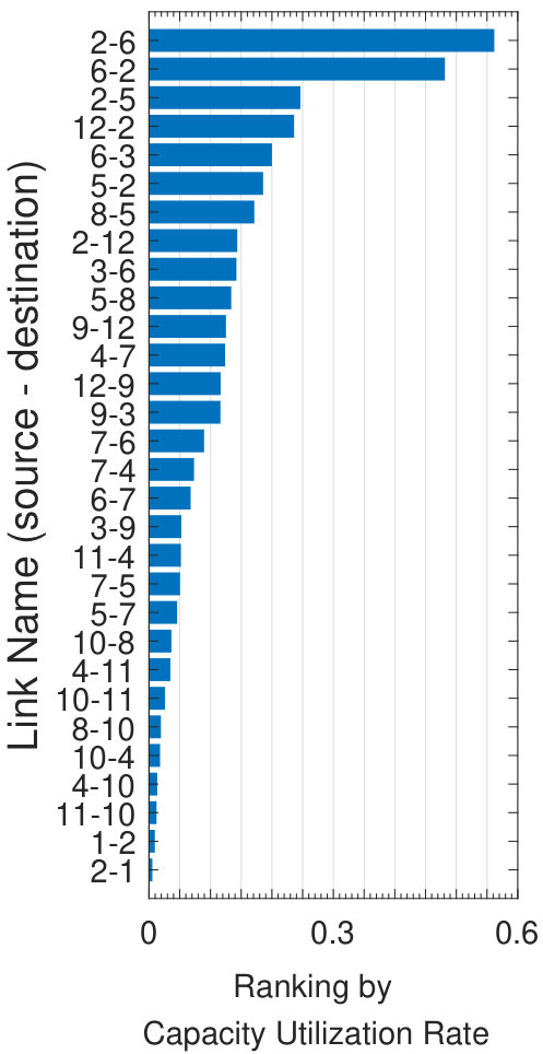 Figure 6
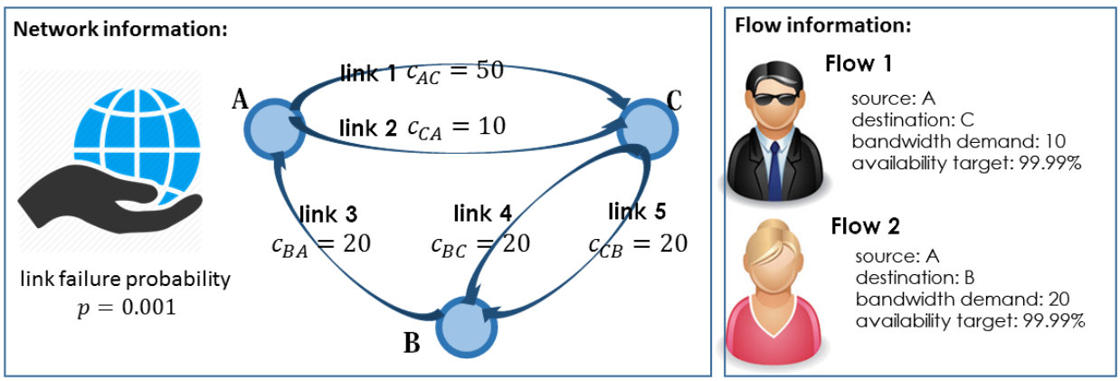 Figure 7
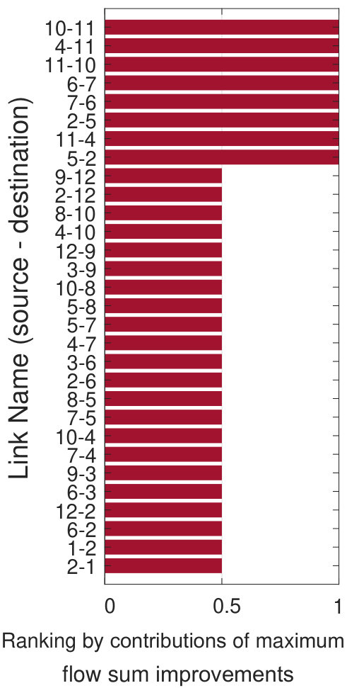 Figure 8
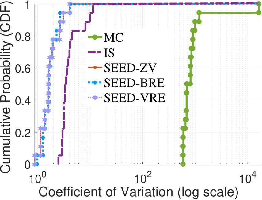 Figure 9
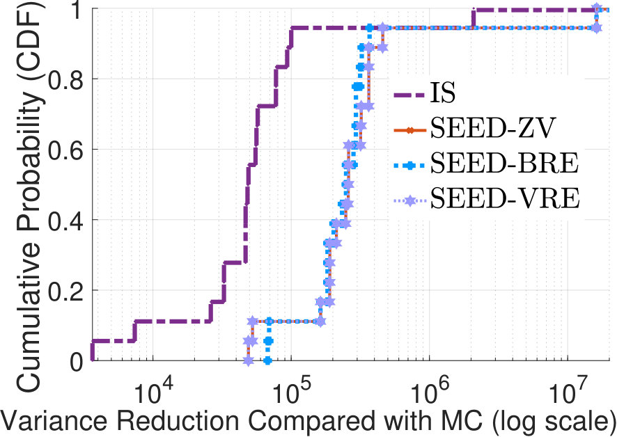 Figure 10
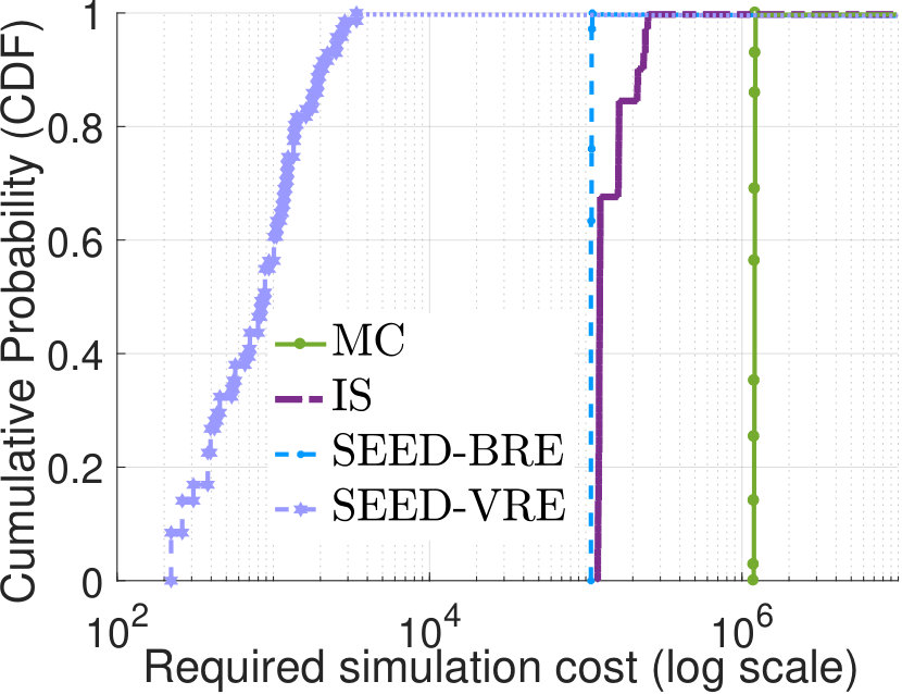 Figure 11
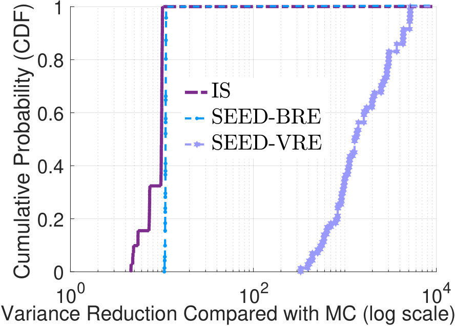 Figure 12
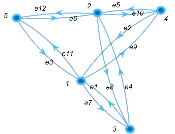 Figure 13
| Monte Carlo Method | Our method (SEED-VRE) | ||||||
|---|---|---|---|---|---|---|---|
| Flow |
Theoretical
Unavailability |
Estimated
Unavailability |
Empirical
Variance |
Number of
Simulations |
Estimated
Unavailability |
Empirical
Variance |
Number of
Simulations |
| 1 | 10,000 | 10 | |||||
| 2 | 10,000 | 10 | |||||
|
Reliability
Measurement |
NCR [7, 8, 9, 17, 18] | MFR [11, 12, 13] | Flow Availability |
|---|---|---|---|
| Definition | node and are connected | max flow from to | flow ’s demand is satisfied |
|
Required
Information |
Topology Information: and . | Topology Information: , and . |
Topology Information: , and ;
Flow Information: and for . |
|
Application
scenarios |
1) Topology design evaluation. |
1) Topology design evaluation;
2) Capacity planning design evaluation. |
1) Topology design evaluation; 2) Capacity planning design evaluation; 3) Sales projection design evaluation. |
| Relationship |
The flow availability is a generalization of network connectivity and maximum flow based reliabilities.
When link capacity for , flow ’s demand is satisfiednode and are connected. When flow set contains only one flow, flow ’s demand is satisfiedmax flow from to . |
||
| Note: Consider in network , there exist node and flow from to with demand . Let vector and denote information of failure probability and capacity across all links. Consider in flow set , each flow is associated with a source , a destination and a demand . | |||
| Notations | Descriptions |
|---|---|
| The number of transportation links and flows. | |
| The th link, where . | |
| , , , | and are ’s failure probability and distribution. and is the distribution induced by . |
| Failure configuration. and () means that the link is down (up). | |
| The th flow, where . | |
| ’s flow information, including source , destination , bandwidth demand and availability target . | |
| Indicator function of traffic engineering simulation. Given , () if the flow fails (succeeds). | |
| is a link set. is a collection of link sets. | |
| , | maps a link set to the failure configuration which satisfies: , ; , . maps a failure configuration to the link set . |
| , | is the collection of link set ’s supersets and is the collection of supersets of all link sets . |
| , the collection of all failure link sets which can result in flow failures. | |
| A SEED is a special link set satisfying: 1) ; 2) , ; 3) , . And is the collection of all SEEDs. |
| 0.49975 | 0.00050 | 0.49975 | |
| 0.25000 | 0.25025 | 0.25000 |
| Full SEED Set | Partial SEED Set | ||||||||
| MC | IS | SEED-ZV | SEED-BRE | SEED-VRE | SEED-ZV | SEED-BRE | SEED-VRE | ||
| Note: Information of flow : 1) the tuple of source, destination and demand ; 2) the full SEED set ; 3) the partial SEED set with good coverage . | |||||||||
| MC | IS | SEED-BRE | |
|---|---|---|---|
| Simulation cost () |
Peer Reviews
No public reviews on file for this paper yet. If you reviewed it on a platform where reviews are public (OpenReview, ICLR, NeurIPS, ICML), you can paste yours below so the community can read it here.
Videos
No videos yet. Explain this paper in a talk, walkthrough, or lecture? Add one.
Taxonomy
TopicsReliability and Maintenance Optimization · Advanced Queuing Theory Analysis · Radiation Effects in Electronics
FAVE: A fast and efficient network Flow AVailability Estimation method with bounded relative error
††thanks: This work is supported in part by the GRF 14200117 and the Huawei Grant.
Tingwei Liu*†, John C.S. Lui∗*
Department of Computer Science & Engineering, The Chinese University of Hong Kong, China*
Email: *†*[email protected], *∗*[email protected]
Abstract
This paper focuses on helping network providers to carry out network capacity planning and sales projection by ans-wering the question: For a given topology and capacity, whether the network can serve current flow demands with high probabili-ties? We name such probability as “flow availability”, and present the flow availability estimation (FAVE) problem, which is a gener-alisation of network connectivity or maximum flow reliability esti-mations. Realistic networks are often large and dynamic, so flow availabilities cannot be evaluated analytically and simulation is often used. However, naive Monte Carlo (MC) or importance sam-pling (IS) techniques take an excessive amount of time. To quickly
estimate flow availabilities, we utilize the correlations among link and flow failures to figure out the importance of roles played by different links in flow failures, and design three “sequential imp-ortance sampling” (SIS) methods which achieve “bounded or even vanishing relative error” with linear computational complexities.
When applying to a realistic network, our method reduces the flow
availability estimation cost by 900 and 130 times compared with MC and baseline IS methods, respectively. Our method can also facilitate capacity planning by providing better flow availability guarantees, compared with traditional methods.
I Introduction
Network capacity planning is the process of ensuring sufficient bandwidth is provisioned so that service-level agreement (SLA) objectives like delay, jitter, loss and routing availability can be satisfied [1]. For the purpose of providing a better end user experience and at the same time, keeping the operation cost at an affordable level, effective capacity planning tools are crucial to network providers. Various systems have been built around this problem, such as Cisco’s MATE [2], Facebook’s Prophet [3], and Google’s backbone capacity planning tool [4].
Motivations of fast flow availability estimations: The above SLA objectives are called the demand of a traffic flow, and the
satisfaction probability of demand is defined as the flow availability. A key concern of capacity planning is in analyzing the effect of network changes or the arising of new flows on the flow demand satisfaction [2]. To illustrate, consider an example that a network provider needs to serve two flows as shown in Fig.1. In this network, each link is associated with a failure probability, say and a capacity ; also, flow routing follows the “max-min fairness” and “shortest path” policies. Each flow has a bandwidth demand, and an availability target (i.e., the lower bound probability that its requested bandwidth needs to be satisfied). The network provider will perform:
- Flow availability testing, i.e., whether flow availability targets can be achieved? E.g., flow 1’s availability target is achieved if it obtains 10 units of bandwidth with a probability no less than .
- Capacity planning, e.g, to improve the network, should the provider add more links between node and , or add a new node so to increase the path diversity?
- **Sales
projection**, e.g., to increase profit, can the provider admit a new
flow 3? Will the network still provide flow availability guarantees if flow 1 requires 20 additional units of bandwidth? All these cases need flow availabilities to see whether the network
(proposed by capacity planning) can serve flow demands (proposed by sales projection). We name the flow availability esti-mation problem as “FAVE”, and give a formal definition later.
For a large realistic network with complex failure patterns,
the flow availability often cannot be evaluated analytically, especially when the traffic scheduling is also considered. Hence, simulation (or sampling) is often used. The Monte Carlo (MC)
method [5], which simulates link failures with real link failure
probabilities, is the most widely used.
Yet, it can be costly for MC to achieve a desired accuracy level, e.g., to estimate flow 2’s availability in Fig.1, by variances collected in Table 1, MC needs at least 3,840 simulation steps to guarantee the 95% confidence interval (CI) width below . To simulate a large network with many flows, it is crucial to find ways to speed up the simulation process.
High level ideas of our work: The flow availability estimation
can be more efficient if flow failures (i.e., flow demands could not be satisfied) happen more frequently by taking a proper distribution to simulate link failures, which is the key idea of “importance sampling (IS)” [6]. We first introduce a baseline IS solution for FAVE using “*the correlation between link failures
and flow failures*” to decide “important links” whose failures are more likely to result in flow failures. We then simulate such links’ failures more often to speed up simulating flow failures. To further improve upon the baseline IS, we show that some link sets’ failures happen more often, and play a role of “root causes” of flow failures. We name such link set as “SEED”. We
utilize “the correlation among link failures” captured by SEEDs
to decide “important link sets” whose failures are more likely
to result in flow failures. We propose three advanced “sequential importance sampling (SIS)” algorithms, among which the SEED-VRE algorithm has the “vanishing relative error (VRE)” and “linear computational complexity”. Table 1 illustrates the computational reduction of our methods: Using only 10 simulation steps, both empirical variance and estimation error are much smaller than that of MC with 10,000 simulation steps. In other words, not only we can speed up simulations, but the network operator is able to achieve a higher accuracy of flow availability estimation without incurring an additional cost.
We emphasize that flow availability estimation can also faci-litate capacity planning: for flows with unachievable availability targets, we show that allocating more capacities for the important links determined by our method would bring a better
flow availability improvement, compared with traditional me-thods to allocate more capacities for links with high utilizations.
Contributions: Our key contribution is in providing efficient and accurate solutions for FAVE. Contributions include:
- •
We formally define the network Flow AVailability Estimation
(FAVE) problem, and show it generalizes the classical network reliability estimation problem [7, 8, 9, 10, 11, 12, 13].
- •
For FAVE with a single flow, we introduce a novel concept of
“SEED” and propose three advanced SIS algorithms which have attractive properties of bounded relative error (BRE) or
VRE with linear computational complexities.
- •
For FAVE with multiple flows, we propose a mixture SIS method which maintains BRE property and linear computa-tional complexity when estimating all flows’ availabilities.
- •
For FAVE with a partial SEED set information, we maintain the BRE and VRE properties of flow availability estimations.
- •
Extensive results show that our methods greatly speed up the flow availability estimation: 1) Given an illustrative network and full SEED sets or partial SEED sets with good coverage, SEED-VRE achieves variance reductions of 360,000 and 7,000 times in the single flow case, and *200,000 and 7 times
*for around 80% flows in the multiple flow case, compared with MC and baseline IS. 2) Given a realistic network and partial SEED sets with poor coverage, SEED-VRE reduces simulation cost by 900 and 130 times for around 80% flows in the multiple flow case, compared with MC and baseline IS.
- •
We demonstrate our methods facilitate capacity planning by providing more accurate network reliability evaluations compared with classical methods, and greater flow availability improvements compared with solely using the link capacity utilization information.
Organizations: Section II introduces related work and some preliminaries. Section III formally defines the FAVE problem. In Section IV, we propose a baseline IS solution for FAVE and
show its error bounds, then we introduce “SEED” and present SEED based SIS solutions with better error bounds and linear
computational complexities. Section V considers more practi-cal issues, e.g., the multiple flows case and partial SEED sets information case. In Section VI, we evaluate our methods on both an illustrative network and a realistic network, i.e., the Abilene network [14]. Section VII shows the utility of our methods in capacity planning. Finally, Section VIII concludes.
II Related Work & Preliminaries
Our work can be viewed as a generalisation of previous work
in estimating network reliability [7, 8, 9, 10, 11, 12, 13] and is related with importance sampling [6]. Here, we briefly review previous rel-evant studies and compare them with our work. We also descr-ibe some concepts so readers can gain a better understanding of sampling methods for the network reliability estimation.
II-A Network Reliability Estimation
The most relevant literatures to our work focus on evaluating network reliability. To design reliable networks, one needs to measure the impact of network failures (e.g., link failures) on
network performances [15]. It is known that the exact computation of network reliability is #P-complete, and computational
complexities of all known algorithms are exponential increasing with the graph scale [16], which makes the problem intractable even for medium sized networks. Hence, most work on network reliability evaluation considers sampling methods to provide reliability estimations, and they can be classified into
“network connectivity” based and “maximum flow” based.
Network connectivity reliability (NCR): NCR is a classical reliability measure adopted by most work [7, 8, 9]. The network
is modelled as a graph where links are either failed or operational, and NCR is measured by the probability that a given set
of nodes are connected when links fail with given probabilities. Authors in [7] take network repair policies into consideration to model link failures, and estimate NCR with the classical MC Authors in [8] combine MC with the particle swarm optimization to handle the NCR problem. To improve the efficiency of MC, authors in [9] apply the IS method and use pre-computed “graph minimal cuts” to approximate the optimal IS estimator.
Maximum flow reliability (MFR): Another line of work [11, 13, 12] generalizes the NCR problem by considering link capac-ities: link capacities are determined by link statuses, i.e., operational, failed or partially failed, which follow certain probability distributions. Given one source and one sink, MFR is defined as the probability that the maximum flow, i.e., the maximum achievable bandwidth from the source to the sink, is above a given threshold. In [11], link capacities are assumed to be continuous and the MC splitting method is applied for the
MFR estimation. Authors in [12] follow the idea of permutating MC and assume all links fail at the beginning and each one of them gets repaired after a random time. Authors in [13] consider estimating MFR with the order minimal cut sets.
Other reliabilities: Some works also study the connection availability [17] and service availability [18], and consider the probability that a connection or service is available. Authors in
[17] evaluate the connection availability by computing the connection probability of a small subset of nodes exactly. Authors in [18] evaluate the service availability by using IS to estimate path availabilities. The problem considered in [17, 18] can be
transformed to a problem of determining the connectivity of certain nodes, where the network topology is given. Hence, [17, 18] are essentially the same with the NCR related work.
II-B Comparisons with Classical Reliability Estimation Work
We consider the “flow availability” as our reliability measure. We first give the definition of the flow demand.
Definition 1**.**
The “demand” of flow is the quality of service
(QoS) requirements decided by ’s SLA objective.
Consider different SLA objectives, the flow demand can be,
for instance, the bandwidth demand, latency demand or packet loss demand, which specifies ’s QoS requirement on bandwidth, transmission latency or packet loss.
To be concrete and so easier to understand, we take the bandwidth demand as an example, and the following analysis works the same for other demands. We define the flow availability as:
Definition 2**.**
For a given topology information, flow information, routing policy and resource allocation policy, the “flow availability” of is the probability that ’s demand is satisfied.
Comparing with the state-of-the-art methods, our methods have the following advantages:
- The flow availability can be applied to evaluate both NCR, given all links have unlimited capacities, and MFR, given the network contains only one flow. Yet, neither NCR nor MFR can address FAVE. To illustrate, consider the example in Fig.1. If link 1 fails, the network is still connected but neither flow 1 nor 2’s demands can be satisfied. Also, the maximum flow from
to still achieves 10 units, but it does not imply flow 1 succeeds, which depends both on resource allocation and routing policies and other competing flows.
- Flow availability can be applied to evaluate not only the reli-ability of network designs, including topology design and capacity planning, but also the feasibility of sales projection. In contrast, NCR only applies to the topology design evaluation and MFR only applies to the capacity planning evaluation, for they utilize solely the (partial) topology information.
To summarize, FAVE generalizes the NCR and MFR estimations and considers a more realistic problem setting. Moreover, it can be applied to evaluate impacts of more factors, e.g., network topology, capacity and flow information on network per-formances, and provides more accurate evaluation results. The detailed comparisons can be found in Table. 2.
II-C Sampling Methods for Network Reliability Estimations
Network reliability estimation problem: Let the network be
modelled as a directional multigraph with nodes
in node set and links in link set . Each link is associated with a tuple with a small probability to
represent ’s failure probability, a capacity , and a status ,
where () means is down (up). Let ,
and be failure probability, capacity and status across all links respectively. , also called the “failure configuration”, is generated by the link failure distribution induced by . There are possible configurations of , which is huge for a large realistic network.
Let be the indicator function of some interested event . According to the reliability definition, can refer to the event
that a subset of nodes are unconnected, or the maximum flow is
below the required threshold, or, in our case, the flow demand is unsatisfied. Given link statuses described by , if is observed and vice versa. The network unreliability, which is the occurrence probability of , can be computed via the following integral in the discrete measure space:
[TABLE]
where means taking the expectation over distribution . Then, the network reliability can be obtained by .
Monte Carlo (MC) simulation: The MC simulation draws failure configurations independently from and estimate with the following MC estimator:
[TABLE]
where is the number of simulation steps and is the th generated failure configuration. As MC generates link statuses by true link failure probabilities (which can be small), it is rare
to observe link failures, and even rarer to observe . This implies that we need a large to gain the desired accuracy.
Importance sampling (IS): To improve the efficiency of MC, IS changes the sampling distribution to increase the occurrence of , and assigns each sample a weight to recover the unbiasedness. Specifically, it replaces Eq.(1) by:
[TABLE]
where is the “importance distribution”. For convenience, denote as the weight. Therefore, the above expectation is estimated by the following IS estimator:
[TABLE]
Estimator efficiency evaluation: An estimator’s efficiency is often measured by its “variance”. Take the MC estimator as an example, its variance is given by:
[TABLE]
where means taking the variance over the distribution . The IS estimator’s variance can be expressed as:
[TABLE]
Note that the MC estimator is a special case of the IS estimator if , . Define as the “one-run variance” of the IS estimator. To achieve a desired estimation
accuracy, the CI width should be bounded by a threshold , i.e.,
, and the simulation cost is , where is a constant decided by the required confidence level. Thus, a small and bounded implies an efficient estimator.
Zero-variance (ZV) importance distribution: The following theorem gives an optimal importance distribution :
Theorem 1** (Zero-variance importance sampling).**
The IS estimator in Eq.(4) can achieve zero-variance, i.e, , if the importance distribution where:
[TABLE]
Remark: Although the ZV property implies a minimum simulation cost, it is non-trivial and sometimes even impossible to compute the ZV importance distribution . Hence, the key of designing an efficient IS estimator lies in the approximation of . As for different applications and problem definitions,
the auxiliary information we can utilize and the way to approximate are different, designing efficient IS estimators are highly challenging and problem-dependent.
III Problem Definition
Consider the network with topology information , as defined in Section II-C. We consider a flow set with flows and each flow is associated with a tuple specifying ’s source , destination , demand and availability target . We also define the following:
Definition 3**.**
A flow fails (succeeds) if its demand is unsatisfied (satisfied), e.g., the allocated bandwidth cannot (can) support its bandwidth demand.
We redefine the function to indicate the network routing:
[TABLE]
where represents the topology information, including a tuple for every link ; represents the flow informa-tion, including a tuple for every flow ; and represent the underlying routing and resource allocation policies, e.g., shortest path policy and max-min fairness policy. Function outputs 1 if the interested flow fails and 0 other-wise. We assume all information in is known, exc-ept link statuses described by . To simplify the expression, let:
[TABLE]
Namely, given all other information, the routing result indicated
by only depends on the failure configuration , which is generated by the link failure distribution induced by .
The unavailability , also called the flow failure probability, of a specific flow can be computed via the integral in Eq.(1). Our goal is to evaluate availabilities of (all) flows in . Yet, the complexity of function and the high dimensionality of the topological space make it impossible to evaluate the flow availability analytically. One alternative is to estimate via simulations. We name the network flow availability estimation problem as “FAVE”. And we can show it generalizes the classical network reliability estimation problem [7, 8, 9, 10, 11, 12, 13].
Theorem 2**.**
The FAVE problem generalizes both the network connectivity based and the maximum flow based network reliability estimation problems.
Remark: Due to the page limit, we only provide the sketch proof of Thm. 6 in this paper and we leave proofs of all other lemmas and theorems in the technical report [19].
In addition to measuring the estimation efficiency with the variance, we also consider two attractive error bound properties:
Definition 4** (Bounded Relative Error).**
An estimator with expectation and variance has the bounded relative error (BRE) property
if , i.e., the coefficient of variation (CV) satisfies .
Definition 5** (Vanishing Relative Error).**
An estimator with expectation and variance has the vanishing relative error (VRE) property
if , i.e., .
Remark: Note that the VRE property is stronger than the BRE property. The variance of MC is , i.e., . This implies that the MC estimator satisfies neither BRE nor VRE property. In the following, we will discuss how to design estimation methods which have above properties.
IV Algorithm Design
We first describe our design for “the single flow case”. We start with a baseline IS design to gain insights for efficient estimations. Then we introduce “SEED” and our SEED methods.
IV-A A Baseline Importance Sampling Design
1) ZV importance distribution approximation: It seems easy to design an IS estimator if we can well approximate in Eq.(7). Yet, the following discussion shows that this is not an easy task. We use the KL divergence to measure the similarity between and its approximation . We derive by:
Theorem 3**.**
Assume the optimal importance distribution in Eq.(7) is approximated by a product form distribution:
[TABLE]
then the KL divergence is minimized when:
[TABLE]
By now, the estimation of becomes a new problem. In fact, even given the exact expressions or
values, the performance of this IS method is still not guaran-teed: minimizing the KL divergence can only lower bound the
estimator’s variance, and the lower bound depends on how well
in Eq.(11) can approximate . To see this, consider the case where a network has 2 nodes connected by 3 parallel links with . The flow fails if link statuses are , or . According to Thm. 3, one possible
importance distribution is . In this case, is not well approximated by in Table 4.
Remark: The above example illustrates that minimizing KL divergence cannot provide the IS method a performance guarantee: sometimes our chosen can be very different from . A major reason is that the baseline IS assumes has the product form in Eq.(10), i.e., it considers link failures are independent and ignores the correlations among them. We will discuss how to improve the design of in later sections.
2) Estimation error bound analysis: The variance bounds of the baseline IS method is given by the following theorem:
Theorem 4**.**
If the IS estimator in Eq.(4) takes in Eq.(11) as its importance distribution, then is bounded by:
[TABLE]
Here is the optimal importance distribution given by Eq.(7).
Remark: Thm. 4 implies that although the variance of baseline IS is upper bounded, it can be worse than the variance of MC. This motivates us to seek for more efficient sampling methods with better error bounds.
IV-B Conditions for Efficient Sampling
In the baseline IS design, link importance distributions
are assumed to be independent. This assumption simplifies the problem, but does not correspond to the reality. Consider the
example in Section IV-A, greatly differs from
, which implies the dependence among
and the correlation of links’ statuses cannot be ignored. Next, we propose our “sequential importance sampling” (SIS) based design and take this correlation into consideration.
1) ZV sequential importance sampling: Let us adapt the ZV importance distribution in Eq.(7) for the SIS method. Denote as the status of the first th links.
Theorem 5**.**
For the FAVE problem, the IS estimator in Eq.(4) achieves the ZV property if the importance distribution for the SIS estimator, where:
[TABLE]
Remark: Different from baseline IS, SIS generates links’ statuses in a sequential manner, which enables its importance distribution to capture the correlation of links’ statuses, i.e., links’ importance distributions are dependent.
2) Conditions for good error bounds: To apply the above SIS estimator, we need to estimate (or approximate) . The following theorem states that the above SIS is robust even if there exists some error when approximating .
Theorem 6** (Conditions for BRE and VRE properties).**
The IS estimator in Eq.(4) has the BRE property if , satisfies:
[TABLE]
and the VRE property if , satisfies:
[TABLE]
Proof: Assume . Otherwise there is no need to generate the corresponding . Then, Eq.(14) is equivalent to:
[TABLE]
where is a constant. Thus, we can derive that:
[TABLE]
[TABLE]
[TABLE]
Namely, BRE property is achieved. As Eq.(15) is a special case
of Eq.(16) by restricting for all , it is similar to show that
Eq.(15) implies , i.e., VRE property is achieved.
Remark: Thm. 6 provides important guidelines to design sampling methods with BRE and VRE properties: the estimation should satisfy the conditions listed in Thm. 6.
IV-C SEED Algorithms
1) SEED set and related definition: Before introducing how to
approximate for the SIS estimator, we first present
some definitions used in the later discussion.
Let be the index set of all links. We use function and for transformations between the failure configuration and the set of failure links :
[TABLE]
For one interested flow, denote the collection of all link sets whose failures can result in the flow failure by:
[TABLE]
Also, denote the collection of all supersets of link set by:
[TABLE]
Accordingly, for a collection of link sets ,
[TABLE]
The probability of the event that “all links in fail” is:
[TABLE]
Definition 6** (SEED).**
Define the SEED as a special link set which satisfies the following conditions:
[TABLE]
We also denote the collection of all SEEDs by .
Definition 7** (Conditional SEED).**
Consider the statuses of some links are specified by , define the conditional SEED (cond-SEED for short) as a special link set satisfying:
[TABLE]
Also, we denote the collection of all cond-SEEDs by .
Examples: We give some examples for the above definitions. Consider the example in Section I, we have . By the definition of SEED, the failure of any subset of a SEED, e.g., or , will not result in flow 1’s failure; and the failure of any superset of a SEED, e.g., , will result in flow 1’s failure. If given the first four links’ statuses by , there is only one cond-SEED .
Next, we use “SEED” and “SEED set” to capture the correlation of link failures and approximate in Thm. 5.
2) SEED based IS algorithms: Thm. 5 presents the optimal importance distribution for the SIS method. We next show
that can be computed exactly via Algorithm 1.
Theorem 7**.**
If failure configurations are generated using SEED-ZV, the estimator in Eq.(4) has the ZV property.
Remark: Though SEED-ZV has the ZV property, it is compu-tationally expensive: as the need for traversing all combinations of cond-SEEDs for each link , the computational complexity is .
Note that there is a tradeoff between estimation accuracy and computational complexity to estimate . Next, we consider sacrificing some estimation accuracy of , i.e., utilize probabilities of the most important cond-SEEDs for estimations (in line 3 of Algorithm 2), and propose SEED-BRE, which has a lower linear computational complexity. We show SEED-BRE has the BRE property by the following theorem.
Theorem 8**.**
If failure configurations are generated using SEED-BRE, the estimator in Eq.(4) has the BRE property.
Remark: The computational complexity of SEED-BRE is only , as it needs to traverse all cond-SEEDs in , for each . The size of decreases when increases.
To further improve estimation accuracy, we utilize the probability sum of cond-SEEDs for estimations (in line 3 of Algo-rithm 3), and propose the SEED-VRE algorithm. We next show that SEED-VRE has the VRE property if link failures are rare.
Theorem 9**.**
When link failure probabilities are small and in the form of . If failure configurations are generated by SEED-VRE, the estimator in Eq.(4) has the VRE property.
Remark: The computational complexity of SEED-VRE is also , as it needs to traverse all the cond-SEED sets in , for each .
By now, we have three SEED algorithms, i.e., SEED-ZV,
SEED-BRE and SEED-VRE, to compute the importance distributions of SIS estimator. They can achieve ZV, BRE and VRE properties respectively, and with the computational complexities , and respectively. However, all above discussions focus on the “single flow case”. Next, we will generalize our methods to handle multiple flows and take other practical issues into consideration.
V Practical Consideration
Previous discussions illustrate that SEED methods work well
in estimating a single flow’s availability with the full informa-
tion of . Next, we consider more practical issues. First, as there are flows in the network, it is costly to design a “customized” estimator for each flow and individually estimate
their availabilities. If the designed estimator works for a group of flows, the computational cost can be reduced significantly. Furthermore, as SEED methods rely on the SEED set which may be difficult to obtain the full information at times, we consider the case that only a partial information of is available, e.g., we only know some frequently observed SEEDs.
V-A Generalization to Multiple Flows Case
To provide efficient and accurate availability estimations for a group of flows at the same time, one possibility is to utilize SEED methods to design a pure importance distribution
for each flow , then take a mixture of these pure distributions with a strategy to simulate link failures:
[TABLE]
To derive such a mixture importance distribution, we take a weighted sum of these pure distributions:
[TABLE]
Here can be viewed as the probability of taking to
generate . Denote as ’s failure probability and
as the one-run variance when taking to estimate ’s failure probability. Next we analyze error bounds of this mixture
sampling strategy, when applying to the multiple flows case.
Theorem 10**.**
Using the mixture sampling strategy in Eq.(27) with pure distributions generated by SEED methods, the IS estimator achieves the BRE property for all flows availability estimations. Specifically, for flow , the estimator’s one-run variance satisfies:
[TABLE]
Remark: Thm. 10 states that, when extending to the multiple flows case, our methods guarantee the estimation efficiency for all flows. Designing proper or even optimal weights is challenging. Online learning is a good approach to find a more efficient weight setting, and we leave this as a future work.
V-B Partial Seed Set Information
At times, it may be difficult to obtain a “full” SEED set , especially when the network is large and flow failures are rare. To provide robust estimations, consider the case that we have only a partial information of , e.g., limited historical data of
flow failures which gives . Denote the cond-SEED set induced by and as . To analyze error bound properties of SEED algorithms, we provide the following lemma.
Lemma 1**.**
Given a partial SEED set , when estimating
: SEED-ZV and SEED-BRE have ZV and BRE properties respectively; assume link failure probabilities are small and follow the form of , SEED-VRE have the VRE property.
Remark: Thm. 5 states that the estimation accuracy depends on
how well is approximated. Given , SEED methods have good error bound properties for they can well approximate . However,
given a partial SEED set , the bias between and should be considered. Let us consider the following two cases:
Good coverage case. SEED methods maintain good error bound properties if has a good coverage, which is defined formally as:
[TABLE]
Here is an example of such a partial SEED set:
[TABLE] 2. 2)
Poor coverage case. may not have a good coverage, e.g.,
without prior knowledge of network and flow failures, . In such case, the SEED set information can be collected via pre-samplings and updated while simulating flow failures.
VI Evaluation of SEED methods
We evaluate our methods on both an illustrative small scale network and a realistic network with topology and traffic matrices extracted from the Abilene network [14]. The simulation cost to guarantee the estimation error (or relative error) below a constant is (or ). Hence, we use one-run variance and coefficients of variation (CV) to quantify the estimation efficiency. The variance reduction, i.e., , can imply the simulation cost reduction, i.e., .
VI-A Experiments on an Illustrative Network
The illustrative network111This is provided so that readers can simulate and validate our methods. demonstrates the “best achievable theoretical improvements” using our method, compared with MC and baseline IS. We start with the single flow case, where full SEED sets or partial SEED sets with good coverage are provided. Then we extend it to the multiple flows case.
Experiment setting: The network is modelled as a directional multigraph with five nodes and 12 links as depicted in Fig.3.
For each link : is uniformly distributed over ( is a small positive number); is uniformly distributed over . The flow set contains 18 flows. For each flow : the source and destination are randomly selected; is the bandwidth demand and uniformly distributed over . We consider traffic engineering follows the shortest path and max-min fairness policies. Note that the above setting provides an instance of network routing function in Eq.(8).
Single flow analysis: We start with the single flow case, and
select one particular flow from the 18 flows. The detailed information of , together with the SEED set information, are introduced in notes of Table 5. We compare our SEED methods with MC and baseline IS. The comparison result, including the expectation , theoretical one-run variance and CV , are summarized in Table 5. Let : given a full SEED set , SEED-BRE and SEED-VRE achieve variance reductions of around 2,000 and 360,000 times compared with MC, and around 45 and 7,000 times compared with baseline IS; given a partial SEED set , our SEED methods estimate flow availabilities with very small biases and much smaller variances, i.e.,
with a small simulation cost, the estimation can be very close to the theoretical value. We also reduce from 0.05 to 0.001, to validate the vanishing property of SEED methods. While
reduces with the decreasing : of MC increases significantly as we have discussed in Section III; of baseline IS is relatively stable; of SEED methods reduces significantly, and of SEED-VRE even achieves a 300 times reduction.
Multiple flows analysis: Next, we take all 18 flows into consi-
deration. Let . We consider an equally weighted sum of
flows’ pure importance distributions as the mixture SIS distri-bution. Fig.3(a) illustrates cumulative distributions of if pure distributions are generated by different methods. With SEED methods, for around 80% flows , which is smaller than the best case of of baseline IS. This demonstrates the BRE property of SEED methods as stated in Thm. 10. Furthermore, both SEED methods and baseline IS, their are 1,000 times smaller than that of MC. To depict the variance reduction
compared with MC much clearer, Fig.3(b) shows cumulative distributions of the variance reduction compared with MC. With SEED methods, more than 80% flows have variance reductions . To better illustrate the effici-ency improvement, Table 6 summarizes simulation costs to guarantee that for 80% flows, “with 95% confident the relative error is less than 0.01”, i.e., .
VI-B Experiments on a Realistic Network
Next, consider a realistic network to demonstrate the “improvements in practice” by using our methods. As it is hard to
obtain the full SEED sets information in the complex realistic
case, simulations on the realistic network can validate the efficiency of SEED methods when estimating all flows’ availabilities, given partial SEED sets with poor coverage property.
Experiment setting: We use the Abilene network [14, 20] with topology and traffic matrices collected by [21]. The network contains 12 nodes and 30 links. The flow set contains 132 aggregated flows: all flows with the same source and destination are aggregated as a single flow222We take the Abilene network as an example and consider aggregated flows due to limitations of the accessible realistic traffic data.. We take each flow’s peak
(99 percentile) throughput [22] as its raw demand. As Abilene has a sufficient capacity to serve raw demands, we double raw demands to see whether the network can still support oversubscribed demands. The routing follows the shortest path policy. The capacity allocation follows the max-min fairness policy, which is also adopted by Google’s B4 backbone network [23].
Multiple flows analysis: We consider all aggregated flows and estimate their availabilities at the same time. Due to the high dimensionality of FAVE in this realistic network, it is costly to obtain theoretical variances of different methods. Thus, we run
each method 10,000 times and use the empirical variance [24] to estimate the one-run variance and compute the simulation cost to guarantee that “with 95% confident the relative error is below 0.01”. Fig.5(a) shows cumulative distribu-tions of by taking the mixture of pure distributions gener-ated by different methods333Due to the exponential complexity, SEED-ZV is not applied in this case.. With SEED-VRE, we find that to achieve the desired accuracy level, for around 60% flows the required simulation costs , and for around 80% flows . Simulation costs for SEED-BRE, baseline IS and MC methods to guarantee 80% flows to achieve the accuracy target are 100,000, 180,000 and 1,260,000, respectively. So the
efficiency is improved by around 900 times via SEED-VRE and 13 times via SEED-BRE, compared with MC. Fig.5(b) illustr-ates cumulative distributions of the variance reduction compared with MC. With SEED methods, 80% of the flows have variance reductions larger than times.
VII Applications in Capacity Planning
Now, we demonstrate the utility of our method in capacity planning on the Abilene network.
Consider the case where a network provider needs to build new links with certain capacities so as to achieve all flow availability targets. For a capacity planning proposal , we can evaluate its feasibility and adopt it if feasible, as follows:
- •
We obtain availability feedbacks of each flow , including a flow availability estimation with upper (lower) confidence bound () computed via empirical variances.
- •
’s availability target is achieved if and unreached if .444We run enough simulations to guarantee . is feasible if all flows’ availability targets are achieved; and infeasible otherwise.
By evaluating flow availabilities, we can not only determine which proposal allows the network to provide better flow availability guarantees, but also utilize flow availability feedbacks for further refinements of infeasible proposals. We consider the following information to refine an infeasible proposal:
- •
Link capacity utilization based: The utilization metric is the
primary metric of interest in capacity planning [1]. Hence, link capacity utilizations can imply the importance of links.
- •
Maximum flow based: The maximum flow value is a widely
adopted network reliability measure [11, 12, 13]. We take the increase of the sum of maximum flows brought by increasing one unit link capacity to measure the importance of links.
- •
SEED based: By testing flow availabilities, we get , the set of flows with unsatisfied availability targets. The number
of failed flows in when fails () can be estimated using SEED algorithms and can imply the importance of links.555As , the probability that flow fails given the first th links’ statues , can be estimated using SEED algorithms, can also be estimated by taking as the first link and let , .
Let the current capacity design of Abilene be the original proposal , and twice the raw demands be flow demands, such that is infeasible. We rank links using the above metrics and summarize rankings in Fig.7. Assume the provider has a budget and only affords to build four new links, each has a capacity of 2.5Gbps and a failure probability of 0.01. Based on rankings in Fig.7, we have three proposals, i.e., , and by taking the top four links in Fig.7, 7 and 7. Fig.7(a) shows flow availability evaluation results. As our method selects links with the largest impact on flow failures, it achieves greater flow availability improvements: in , flow availabilities of around 80% of the flows reach 99.9%.
Insights 1: Improper capacity planning offers little help on improving flow availabilities. E.g., although maximizes the sum of maximum flows, it does not consider the distribution of traffic demands across the network, and thus only brings little improvements on flow availabilities.
Insights 2: Link utilization is not always the best indicator of capacity planning. With the shortest path routing policy, link
has a high capacity utilization if many flows’ shortest paths go through it. Yet, if it is easy to find some alternate link when fails, ’s failure will not result in flow failures and so is not
the most important if aiming at improving flow availabilities.
VIII Conclusion
In this paper, we propose fast and accurate methods in solving the FAVE problem. We introduce the concept of “SEED” to
determine the importance of roles played by different links in flow failures, and propose three SEED based SIS methods which achieve BRE and VRE properties with linear computational complexities. To provide robust and scalable estimations, we extend FAVE to the multiple flows case and partial SEED set case, and our methods maintain the estimation efficiency. We apply our methods on both an illustrative network and a realistic network, and our methods reduce the simulation cost by around 900 and 130 times compared with MC and baseline IS methods on the Abilene network. We show that our method facilitates capacity planning by providing more accurate network reliability estimations compared with classical methods, and greater flow availability improvements compared with solely using link capacity utilizations for capacity planning.
The reference list from the paper itself. Each links out to its DOI / PubMed record.
- 1[1] Cisco.Com, “Best practices in core network capacity planning,” https://communities.cisco.com/docs/DOC-35673 , 2013.
- 2[2] ——, “Planning and designing networks with the Cisco MATE portfolio,” https://communities.cisco.com/docs/DOC-36973 , 2013.
- 3[3] S. J. Taylor and B. Letham, “Prophet: forecasting at scale,” https://research.fb.com/prophet-forecasting-at-scale/ , 2017.
- 4[4] A. K. Bangla, A. Ghaffarkhah et al. , “Capacity planning for the Google backbone network,” in Proc. ISMP , 2015.
- 5[5] J. M. Hammersley and D. C. Handscomb, “The general nature of Monte Carlo methods,” in Monte Carlo Methods , 1964, pp. 1–9.
- 6[6] P. W. Glynn and D. L. Iglehart, “Importance sampling for stochastic simulations,” Manag. Sci. , 1989.
- 7[7] Y. Jiang, R. Li et al. , “The method of network reliability and availability simulation based on Monte Carlo,” in Proc. IEEE ICQR 2MSE , 2012.
- 8[8] W. C. Yeh, Y. C. Lin et al. , “A particle swarm optimization approach based on Monte Carlo simulation for solving the complex network reliability problem,” IEEE Trans. Rel. , 2010.